Variable Selection in High-dimensional Varying-coefficient Models with Global Optimality

Variable Selection in High-dimensional Varying-coefficient Models

with Global Optimality

Lan Xue [email protected]

Department of Statistics Oregon State University Corvallis, OR 97331-4606, USA

Annie Qu [email protected]

Department of Statistics

University of Illinois at Urbana-Champaign Champaign, IL 61820-3633, USA

Editor:Xiaotong Shen

Abstract

The varying-coefficient model is flexible and powerful for modeling the dynamic changes of re-gression coefficients. It is important to identify significant covariates associated with response variables, especially for high-dimensional settings where the number of covariates can be larger than the sample size. We consider model selection in the high-dimensional setting and adopt differ-ence convex programming to approximate theL0penalty, and we investigate the global optimality properties of the varying-coefficient estimator. The challenge of the variable selection problem here is that the dimension of the nonparametric form for the varying-coefficient modeling could be infinite, in addition to dealing with the high-dimensional linear covariates. We show that the proposed varying-coefficient estimator is consistent, enjoys the oracle property and achieves an op-timal convergence rate for the non-zero nonparametric components for high-dimensional data. Our simulations and numerical examples indicate that the difference convex algorithm is efficient using the coordinate decent algorithm, and is able to select the true model at a higher frequency than the least absolute shrinkage and selection operator (LASSO), the adaptive LASSO and the smoothly clipped absolute deviation (SCAD) approaches.

Keywords: coordinate decent algorithm, difference convex programming, L0- regularization,

large-psmall-n, model selection, nonparametric function, oracle property, truncatedL1penalty

1. Introduction

High-dimensional data occur very frequently and are especially common in biomedical studies in-cluding genome studies, cancer research and clinical trials, where one of the important scientific interests is in dynamic changes of gene expression, long-term effects for treatment, or the progres-sion of certain diseases.

In the case where some of the predictor variables are redundant, the varying-coefficient model might not be able to produce an accurate and efficient estimator. Model selection for significant pre-dictors is especially critical when the dimension of covariates is high and possibly exceeds the sam-ple size, but the number of nonzero varying-coefficient components is relatively small. This is be-cause even a single predictor in the varying-coefficient model could be associated with a large num-ber of unknown parameters involved in the nonparametric functions. Inclusion of high-dimensional redundant variables can hinder efficient estimation and inference for the non-zero coefficients.

Recent developments in variable selection for varying-coefficient models include Wang, Li and Huang (2008) and Wang and Xia (2009), where the dimension of candidate models is finite and smaller than the sample size. Wang, Li and Huang (2008) considered the varying-coefficient model in a longitudinal data setting built on the SCAD approach (Fan and Li, 2001; Fan and Peng, 2004), and Wang and Xia (2009) proposed the use of local polynomial regression with an adaptive LASSO penalty. For the high-dimensional case when the dimension of covariates is much larger than the sample size, Wei, Huang and Li (2011) proposed an adaptive group LASSO approach using B-spline basis approximation. The SCAD penalty approach has the advantages of unbiasedness, sparsity and continuity. However, the SCAD approach involves non-convex optimization through local linear or quadratic approximations (Hunter and Li, 2005; Zou and Li, 2008), which is quite sensitive to the initial estimator. In general, the global minimum is not easily obtained for non-convex function optimization. Kim, Choi and Oh (2008) have improved SCAD model selection using the difference convex (DC) algorithm (An and Tao, 1997; Shen et al., 2003). Still, the existence of global opti-mality for the SCAD has not been investigated for the case that the dimension of covariates exceeds the sample size. Alternatively, the adaptive LASSO and the adaptive group LASSO approaches are easier to implement due to solving the convex optimization problem. However, the adaptive LASSO algorithm requires the initial estimators to be consistent, and such a requirement could be difficult to obtain in high-dimensional settings.

Indeed, obtaining consistent initial estimators of the regression parameters is more difficult than the model selection problem when the dimension of covariates exceeds the sample size, since if the initial estimator is already close to the true value, then performing model selection is much less challenging. So far, most model selection algorithms rely on consistent LASSO estimators as initial values. However, the irrepresentable assumption (Zhao and Yu, 2006) to obtain consistent LASSO estimators for high-dimensional data is unlikely to be satisfied, since most of the covariates are correlated. When the initial consistent estimators are no longer available, the adaptive LASSO and the SCAD algorithm based on either local linear or quadratic approximations are likely to fail.

effi-cient. This is reflected in that the proposed model selection performs better than existing approaches such as SCAD in the high-dimensional case, based on our simulation and as applied to HIV AIDs data, with a much higher frequency of choosing the correct model. The improvement is especially significant when the dimension of covariates is much higher than the sample size.

We derive model selection consistency for the proposed method and show that it possesses the oracle property when the dimension of covariates exceeds the sample size. Note that the theo-retical derivation of asymptotic properties and global optimality results are rather challenging for varying-coefficient model selection, as we are dealing with an infinite dimension of the nonpara-metric component in addition to the high-dimensional covariates. In addition, the optimal rate of convergence for the non-zero nonparametric components can be achieved in high-dimensional varying-coefficient models. The theoretical techniques applied in this project are innovative as there is no existing theoretical result on global optimality for high-dimensional model selection in the varying-coefficient model framework.

The paper is organized as follows. Section 2 provides the background of varying-coefficient models. Section 3 introduces the penalized polynomial spline procedure for selecting varying-coefficient models when the dimension of covariates is high, provides the theoretical properties for model selection consistency and establishes the relationship between the oracle estimator and the global and local minimizers. Section 4 provides tuning parameter selection, and the coordinate decent algorithm for model selection implementation. Section 5 demonstrates simulations and a data example for high-dimensional data. The last section provides concluding remarks and discussion.

2. Varying-coefficient Model

Let (Xi,Ui,Yi),i=1, . . . ,n, be random vectors that are independently and identically distributed as(X,U,Y), whereX= (X1, . . . ,Xd)T and a scalarU are predictor variables, andY is a response variable. The varying-coefficient model (Hastie and Tibshirani, 1993) has the following form:

Yi= d

∑

j=1

βj(Ui)Xi j+εi, (1)

whereXi jis the jth component ofXi,βj(·)’s are unknown varying-coefficient functions, andεiis a random noise with mean 0 and finite varianceσ2_{.The varying-coefficient model is flexible in that the} responses are linearly associated with a set of covariates, but their regression coefficients can vary with another variableU. We will callU the index variable andXthe linear covariates. In practice, some of the linear covariates may be irrelevant to the response variable, with the corresponding varying-coefficient functions being zero almost surely. The goal of this paper is to identify the irrelevant linear covariates and estimate the nonzero coefficient functions for the relevant ones.

In many applications, such as microarray studies, the total number of the available covariatesd

can be much larger than the sample sizen, although we assume that the number of relevant ones is fixed. In this paper, we propose a penalized polynomial spline procedure in variable selection for the varying-coefficient model where the number of linear covariates d is much larger than n. The proposed method is easy to implement and fast to compute. In the following, without loss of generality, we assume there exists an integerd0such that 0<E

h

β2 j(U)

i

<∞for j=1, . . . ,d0,and

Ehβ2 j(U)

i

3. Model Selection in High-dimensional Data

In our estimation procedure, we first approximate the smooth functionsβj(·) d_j=1in (1) by poly-nomial splines. SupposeU takes values in [a,b]with a<b.Letυj be a partition of the interval [a,b],withNninterior knots

υj=a=υj,0<υj,1<· · ·<υj,Nn <υj,Nn+1=b .

Using υj as knots, the polynomial splines of order p+1 are functions which are p-degree (or less) of polynomials on intervals[υj,i,υj,i+1),i=0, . . . ,Nn−1,and[υj,Nn,υj,Nn+1], and have p−1

continuous derivatives globally. We denote the space of such spline functions byϕj. The advantage of polynomial splines is that they often provide good approximations of smooth functions with only a small number of knots.

LetBjl(·) Jn

l=1be a set of B-spline bases ofϕjwithJn=Nn+p+1. Then for j=1, . . . ,d,

βj(·)≈sj(·) = Jn

∑

l=1

γjlBjl(·) =γTjBj(·),

whereγj = (γj1, . . . ,γjJn)

T _{is a set of coefficients, andB}

j(·) = (Bj1(·), . . . ,BjJn(·))

T _{are B- spline}

bases. The standard polynomial spline method (Huang, Wu and Zhou, 2002) estimates the coeffi-cient functionsβj(·)

d

j=1by spline functions which minimize the sum of squares

e

β1, . . . ,eβd

= argmin sj∈ϕj,j=1,...,d

1 2n

n

∑

i=1

"

Yi− d

∑

j=1

sj(Ui)Xi j

#2 .

Equivalently, in terms of B-spline basis, it estimatesγ= γT 1, . . . ,γTd

T by

eγ= eγT 1, . . . ,eγTd

T

= argmin

γj,j=1,...,d

1 2n

n

∑

i=1

"

Yi− d

∑

j=1

γT jZi j

#2

, (2)

whereZi j=Bj(Ui)Xi j= (Bj1(Ui)Xi j, . . . ,BjJn(Ui)Xi j)

T

.However, the standard polynomial spline approach fails to reduce model complexity when some of the linear covariates are redundant, and furthermore is not able to obtain parameter estimation when the dimension of modeldis larger than the sample sizen.Therefore, to perform simultaneous variable selection and model estimation, we propose minimizing the penalized sum of squares

Ln(s) = 1 2n

n

∑

i=1

"

Yi− d

∑

j=1

sj(Ui)Xi j

#2 +λn

d

∑

j=1

pn

sj

_n, (3)

wheres=s(·) = (s1(·), . . . ,sd(·))T,and

sj n=

∑n_i=1s2_j(Ui)Xi j2/n

1/2

is the empirical norm. In terms of the B-spline basis, (3) is equivalent to

Ln(γ) = 1 2n

n

∑

i=1

"

Yi− d

∑

j=1

γT jZi j

#2 +λn

d

∑

j=1

where γj

Wj =

q

γT

jWjγj with Wj = n

∑

i=1

Zi jZTi j/n. The formulation (3) is quite general. In

particular, for a linear model with βj(u) =βj and the linear covariates being standardized with

∑ni=1Xi j/n=0 and ∑ni=1Xi j2/n=1 for j=1, . . . ,d,(3) reduces to a family of variable selection methods for linear models with the penalty pn

sj

n

=pn

βj

.For instance, the L1 penalty

pn(|β|) =|β|results in LASSO (Tibshirani, 1996), and the smoothly clipped absolute deviation penalty results in SCAD (Fan and Li, 2001). In this paper, we consider a rather different approach for the penalty function such that

pn(β) =p(β,τn) =min(|β|/τn,1), (5)

which is called a truncatedL1−penalty (TLP) function, as proposed in Shen, Pan and Zhu (2012). In (5), the additional tuning parameterτn is a threshold parameter determining which individual components are to be shrunk towards to zero, or not. As pointed out by Shen, Pan and Zhu (2012), the TLP corrects the bias of the LASSO induced by the convex L1-penalty and also reduces the computational instability of theL0-penalty. The TLP is able to overcome the computation difficulty for solving non-convex optimization problems by applying difference convex programming, which transforms non-convex problems into convex optimization problems. This leads to significant com-putational advantages over its smooth counterparts, such as the SCAD (Fan and Li, 2001) and the minimum concavity penalty (MCP, Zhang, 2010). In addition, the TLP works particularly well for high-dimensional linear regression models as it does not depend on initial consistent estimators of coefficients, which could be difficult to obtain whend is much larger thann. In this paper, we will investigate the local and global optimality of the TLP for variable selection in varying-coefficient models in the high-dimensional case whend≫n, andngoes to infinity.

Here we obtainbγby minimizingLn(γ)in (4). As a result, for anyu∈[a,b],the estimators of the unknown varying-coefficient functions in (1) are given as

b

βj(u) = Jn

∑

l=1

bγjlBjl(u), j=1, . . . ,d. (6)

Leteγ(o)_{= (eγ}

1, . . . ,eγd0,0, . . . ,0)

T

be the oracle estimator with the first d0elements being the stan-dard polynomial estimator (2) of the true model consisting of only the first d0 covariates. The following theorems establish the asymptotic properties of the proposed estimator. We only state the main results here and relegate the regularity conditions and proofs to the Appendix.

Theorem 1 Let An(λn,τn) be the set of local minima of (4). Under conditions (C1-C7) in the

Appendix, the oracle estimator is a local minimizer with probability tending to 1, that is,

Peγ(o)_∈A

n(λn,τn)

→1,

as n→∞.

Theorem 2 Letbγ= (bγ1, . . . ,bγd)T be the global minima of (4). Under conditions (C1-C6), (C8) and

(C9) in the Appendix, the estimator by minimizing (4) enjoys the oracle property, that is,

Pbγ=eγ(o)→1,

Theorem 1 guarantees that the oracle estimator must fall into the local minima set. Theorem 2, in addition, provides sufficient conditions such that the global minimizer by solving the non-convex objective function in (4) is also the oracle estimator.

In addition to the results of model selection consistency, we also establish the oracle property for the non-zero components of the varying-coefficients. For any u∈[a,b], let bβ(1)_{(u) =}

b

β1(u), . . . ,bβd0(u)

T _{be the estimator of the firstd}

0varying-coefficient functions which are non-zero and are defined in (6) withbγbeing the global minima of (4). Theorem 3 establishes the asymp-totic normality ofbβ(1)_{(u)with the optimal rate of convergence.}

Theorem 3 Under conditions (C1) - (C6), (C8) and (C9) given in the Appendix, and if

limNnlogNn/n=0, then for any u∈[a,b],

n

Vbβ(1)(u)o−1/2bβ(1)(u)−β(₀1)(u)→N(0,I)

in distribution, whereβ(₀1)(u) = (β01(u), . . . ,β0d0(u))

T_{,Iis a d}

0×d0identity matrix, and

Vbβ(1)(u)=B(1)(u) n

∑

i=1

A(_i1)TA(_i1)

!−1

B(1)(u) =Op(Nn/n),

in which B(1)(u) = BT₁(u), . . . ,BT_d0(u)T, and A(_i1) = BT₁(Ui)Xi1, . . . ,BT_d0(Ui)Xid0

T

with

BT

j (Ui)Xi j = (Bj1(Ui)Xi j, . . . ,BjJn(Ui)Xi j). 4. Implementation

In this section, we extend the difference convex (DC) algorithm of Shen, Pan and Zhu (2012) to solve the nonconvex minimization in (4) for varying-coefficient models. In addition, we provide the tuning parameter selection criteria.

4.1 An Algorithm

The idea of the DC algorithm is to decompose a non-convex object function into a difference be-tween two convex functions. Then the final solution is obtained iteratively by minimizing a se-quence of upper convex approximations of the non-convex objective function. Specifically, we decompose the penalty in (5) as pn(β) = pn1(β)−pn2(β),where pn1(β) =|β|/τn and pn2(β) = max(|β|/τn−1,0).Note that both pn1(·)andpn2(·)are convex functions. Therefore, we can de-compose the non-convex objective functionLn(γ)in (4) as a difference between two convex func-tions,

Ln(γ) =Ln1(γ)−Ln2(γ), where

Ln1(γ) = 1 2n

n

∑

i=1

"

Yi− d

∑

j=1

γT_jZi j

#2 +λn

d

∑

j=1

pn1

γj

Wj

,

Ln2(γ) = λn d

∑

j=1

pn2

γj

Wj

Let_bγ(0) _{be an initial value. From our experience, the proposed algorithm does not rely on initial} consistent estimators of coefficients so we have usedbγ(0)_{=0in the implementations. At iteration}

m,we setL(nm)(γ), an upper approximation ofLn(γ), equal to

Ln1(γ)−

"

Ln2

bγ(m−1)_+λ

n d

∑

j=1

γj

W j−

bγ(_jm−1)

W j

p′_n2

bγ(_jm−1)

W j # ≈ 1 2n n

∑

i=1

"

Yi− d

∑

j=1

γT jZi j

#2 +λn

τn d

∑

j=1

γj

W j

I _bγ(_jm−1) W j

≤τn

!

−Ln2

bγ(m−1)+λn

τn d

∑

j=1

bγ(_jm−1)

W j

I _bγ(_jm−1) W j

>τn

!

,

wherep′_{n2 b}γ(_jm−1) W j

!

= 1

τnI(

bγ(_jm−1)

W j

>τn)is the subgradient ofpn2.Since the last two terms of the above equation do not depend onγ,therefore at iterationm,

bγ(m)= argmin

γj,j=1,...,d

   1 2n n

∑

i=1

"

Yi− d

∑

j=1

γT_jZi j

#2 +

d

∑

j=1

λn j

γj W j  

, (7)

where λn j = λ_τnnI bγ(jm−1)

W j

≤τn

!

. Then it reduces to a group lasso with component-specific

tuning parameterλn j. It can be solved by applying the coordinate-wise descent (CWD) algorithm as in Yuan and Lin (2006). To be more specific, let Z∗_{i j} =W−1_j /2Zi j andγ∗j =W

1/2

j γj.Then the minimization problem in (7) reduces to

bγ∗(m)_{= argmin}

γ∗ j,j=1,...,d

   1 2n n

∑

i=1

"

Yi− d

∑

j=1

γ∗T j Z∗i j

#2 +λn j

d

∑

j=1

γ∗_j2

 

. (8)

Then the CWD algorithm minimizes (8) in each component while fixing the remaining components at their current value. For the jth component,_bγ∗_j(m)is updated by

γ∗_j(m)= 1−λn j

Sj 2 ! +

Sj, (9)

where Sj = Z∗jT

Y−Z∗γ∗₋(m_j ) with γ₋∗(m_j ) = γ∗₁(m)T, . . . ,γ∗_j−1(m)T,0T,γ∗_j+(m₁)T, . . . ,γ∗_d(m)TT,

Z∗_j =Z∗_1j, . . . ,Z∗_{n j}T,Z∗= Z∗₁, . . . ,Z∗_dand(x)₊=xI_{x≥0}.The solution to (8) can therefore be obtained by iteratively applying Equation (9) to j=1, . . . ,duntil convergence.

obtain the sparsest solution through tuning the additional thresholding parametersτn. The involve-ment of the additional tuning ofτnmakes the TLP a flexible optimization procedure.

The minimization in (4) can achieve the global minima if the leading convex function can be ap-proximated, and it is called the outer approximation method (Breiman and Cutler, 1993). However, it has a slower convergence rate. Here we approximate the trailing convex function with fast com-putation, and it leads to a good local minimum if it is not global (Shen, Pan and Zhu, 2012). It can achieve the global minimizer if it is combined with the branch-and-bound method (Liu, Shen and Wong, 2005), which searches through all the local minima with an additional cost in computation. This contrasts to the SCAD or adaptive LASSO approaches which are based on local approxima-tion. Achieving the global minimum is particularly important if the dimension of covariates is high, as the number of possible local minima increases dramatically as pincreases. Therefore, any local approximation algorithm which relies on initial values likely fails.

4.2 Tuning Parameter Selection

The performance of the proposed spline TLP method crucially depends on the choice of tuning parameters. One needs to choose the knot sequences in the polynomial spline approximation and

λn,τnin the penalty function. For computation convenience, we use equally spaced knots with the number of interior knotsNn= [n1/(2p+3)], and select onlyλn,τn. A similar strategy for knot selection can also be found in Huang, Wu and Zhou (2004), and Xue, Qu and Zhou (2010). Letθn= (λn,τn) be the parameters to be selected. For faster computation, we use K-fold cross-validation to select

θn, with K=5 in the implementation. The full data T is randomly partitioned into K groups of about the same size, denoted asTv , forv=1, . . . ,K. Then for eachv, the dataT−Tv is used for estimation andTv is used for validation. For any givenθn, let ˆβ(_jv)(·,θn)be the estimators ofβj(·) using the training dataT−Tvfor j=1, . . . ,d. Then the cross-validation criterion is given as

CV(θn) = K

∑

v=1i

∑

∈Tv

(

Yi− d

∑

j=1 ˆ

β(_jv)(Ui,θn)Xi j

)2 .

We select ˆθnby minimizing CV(θn).

5. Simulation and Application

In this section, we conduct simulation studies to demonstrate the finite sample performance of the proposed method. We also illustrate the proposed method with an analysis of an AIDS data set. The total average integrated squared error (TAISE) is evaluated to assess estimation accuracy. Letbβ(r)_be the estimator of a nonparametric functionβin ther-th (1≤r≤R) replication and{um}

ngrid

m=1be the grid points wherebβ(r)_{is evaluated. We define AISE}b_β= 1

R∑ R

r=1ngrid1 ∑

ngrid

m=1

n

β(um)−bβ(r)(um)

o2 ,

and TAISE=∑d_l=1AISEbβl

5.1 Simulated Example

We consider the following varying-coefficient model

Yi= d

∑

j=1

βj(Ui)Xi j+εi,i=1, . . . ,200, (10)

where the index variablesUi are generated from a Uniform[0,1],and the linear covariatesXi are generated from a multivariate normal distribution with mean 0 andCov(Xi j,Xi j′) =0.5|j−j

′

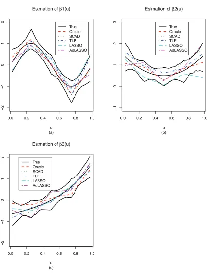
|_,the noisesεi are generated from a standard normal distribution, and the coefficient functions are of the forms

β1(u) =sin(2πu), β2(u) = (2u−1)2+0.5, β3(u) =exp(2u−1)−1,

andβj(u) =0 for j=4, . . . ,d. Therefore only the first three covariates are relevant for predicting the response variable, and the rest are null variables and do not contribute to the model prediction. We consider the model (10) withd=10, 100,200, or 400 to examine the performance of model selection and estimation whendis smaller than, close to, or exceeds the sample size.

We apply the proposed varying-coefficient TLP with a linear spline. The simulation results based on the cubic spline are not provided here as they are quite similar to those based on the linear spine. The tuning parameters are selected using the five-fold cross-validation procedure as described in Section 4.2. We compare the TLP approach to a penalized spline procedure with the SCAD penalty, the group LASSO (LASSO) and the group adaptive LASSO (AdLASSO) as described in Wei, Huang and Li (2011). For the SCAD penalty, the first order derivative ofpn(·)in (4) is given asp′_n(θ) =I(θ≤λn) +(

aλn−θ)+

(a−1)λn I(θ>λn), and we seta=3.7 as in Fan and Li (2001).

For all procedures, we select the tuning parameters using a five-fold cross-validation procedure for fair comparison. To assess the estimation accuracy of the penalized methods, we also consider the standard polynomial spline estimations of the oracle model (ORACLE). The oracle model only contains the first three relevant variables and is only available in simulation studies where the true information is known.

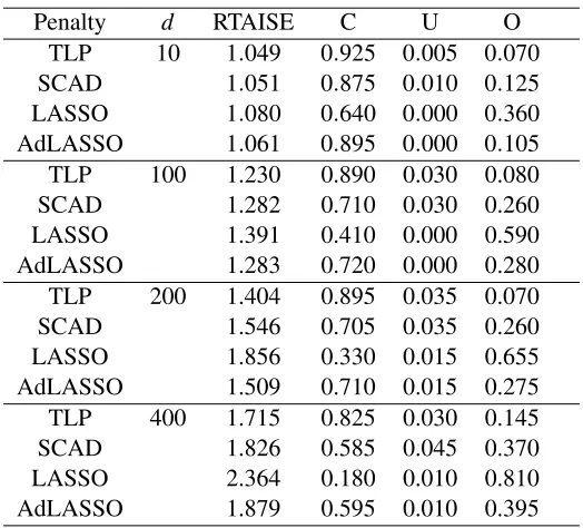
Table 1 summarizes the simulation results. It gives the relative TAISEs (RTAISE) of the penal-ized spline methods (TLP, SCAD, LASSO, AdLASSO) to the ORACLE estimator. It also reports the percentage of correct fitting(C), underfitting(U) and overfitting(O) over 200 simulation runs for the penalized methods. Whend=10, the performance of the TLP, SCAD, LASSO and AdLASSO are comparable, with TLP being slightly better the rest. But as the dimensiondincreases, Table 1 clearly shows that the TLP outperforms the other procedures. The percentage of correct fitting for SCAD, LASSO and AdLASSO decreases significantly more whend increases, while the perfor-mance of the TLP is relatively stable asdincreases. For example, whend=400, the correct fitting is 82.5% for TLP versus 58.5% for SCAD, 18% for LASSO, and 59.5% for AdLASSO in the linear spline. In addition, SCAD, LASSO and AdLASSO also tend to over-fit the model whendincreases, for example, whend=400, the over-fitting rate is 37% for SCAD, 81% for LASSO, and 39.5% for AdLASSO versus 14.5% for TLP in the linear spline.

In terms of estimation accuracy, Table 1 shows that the RTAISE of the TLP is close to 1 when

Penalty d RTAISE C U O TLP 10 1.049 0.925 0.005 0.070 SCAD 1.051 0.875 0.010 0.125 LASSO 1.080 0.640 0.000 0.360 AdLASSO 1.061 0.895 0.000 0.105 TLP 100 1.230 0.890 0.030 0.080 SCAD 1.282 0.710 0.030 0.260 LASSO 1.391 0.410 0.000 0.590 AdLASSO 1.283 0.720 0.000 0.280 TLP 200 1.404 0.895 0.035 0.070 SCAD 1.546 0.705 0.035 0.260 LASSO 1.856 0.330 0.015 0.655 AdLASSO 1.509 0.710 0.015 0.275 TLP 400 1.715 0.825 0.030 0.145 SCAD 1.826 0.585 0.045 0.370 LASSO 2.364 0.180 0.010 0.810 AdLASSO 1.879 0.595 0.010 0.395

Table 1: Simulation results for model selection based on various penalty functions: Relative total averaged integrated squared errors (RTAISEs) and the percentages of correct-fitting (C), under-fitting (U) and over-fitting (O) over 200 replications.

those with TAISE being the median of the 200 TAISEs from the simulations. Also plotted are the point-wise 95% confidence intervals from the ORACLE estimation, with the point-wise lower and upper bounds being the 2.5% and 97.5% sample quantiles of the 200 ORACLE estimates. Figure 1 shows that the proposed TLP method estimates the coefficient functions reasonably well. Compared with the SCAD, LASSO and AdLASSO, the TLP method gives better estimation in general, which is consistent with the RTAISEs reported in Table 1.

5.2 Application to AIDS Data

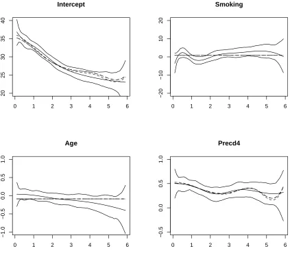
In this subsection, we consider the AIDs data in Huang, Wu and Zhou (2004). The data set consists of 283 homosexual males who were HIV positive between 1984 and 1991. Each patient was sched-uled to undergo measurements related to their disease at a semi-annual base visit, but some of them missed or rescheduled their appointments. Therefore, each patient had different measurement times during the study period. It is known that HIV destroys CD4 cells, so by measuring CD4 cell counts and percentages in the blood, patients can be regularly monitored for disease progression. One of the study goals is to evaluate the effects of cigarette smoking status (Smoking), with 1 as smoker and 0 as nonsmoker; pre-HIV infection CD4 cell percentage (Precd4); and age at HIV infection (age), on the CD4 percentage after infection. Letti j be the time in years of the jth measurement for theith individual after HIV infection, andyi j be the CD4 percentage of patientiat timeti j. We consider the following varying-coefficient model

0.0 0.2 0.4 0.6 0.8 1.0

−2

−1

0

1

2

Estmation of β1(u)

u

True Oracle SCAD TLP LASSO AdLASSO

(a)

0.0 0.2 0.4 0.6 0.8 1.0

−1

0

1

2

3

Estmation of β2(u)

u True Oracle SCAD TLP LASSO AdLASSO

(b)

0.0 0.2 0.4 0.6 0.8 1.0

−2

−1

0

1

2

Estmation of β3(u)

u True Oracle SCAD TLP LASSO AdLASSO

(c)

We apply the proposed penalized cubic spline (p=3) with TLP, SCAD, LASSO and Adaptive LASSO penalties to identify the non-zero coefficient functions. We also consider the standard polynomial spline estimation of the coefficient functions. All four procedures selected two non-zero coefficient functionsβ0(t)andβ3(t), indicating that Smoking and Age have no effect on the CD4 percentage. Figure 2 plots the estimated coefficient functions from the standard cubic spline, SCAD, TLP, LASSO and Adaptive LASSO approaches. For the standard cubic spline estimation, we also calculated the 95% point-wise bootstrap confidence intervals for the coefficient functions based on 500 bootstrapped samples.

0 1 2 3 4 5 6

20

25

30

35

40

Intercept

0 1 2 3 4 5 6

−20

−10

0

10

20

Smoking

0 1 2 3 4 5 6

−1.0

−0.5

0.0

0.5

1.0

Age

0 1 2 3 4 5 6

−0.5

0.0

0.5

1.0

Precd4

In this example, the dimension of the linear covariates is rather small. In order to evaluate a more challenging situation with higher dimension ofd, we introduced an additional 100 redundant linear covariates, which are artificially generated from a Uniform[0,1]distribution independently. We then apply the penalized spline with TLP, SCAD, LASSO or Adaptive LASSO penalties to the augmented data set. We repeated this procedure 100 times. For the three observed variables in model (11), all four procedures always select the Precd4 and never select Smoking and Age. For the 100 artificial covariates, the TLP selects at least one of these artificial covariates only 8 times, while LASSO, Adaptive LASSO, and SCAD select 28, 27, and 42 times respectively. Clearly, LASSO, Adaptive LASSO and SCAD tend to overfit the model and select many more null variables in this data example. Note that our analysis does not incorporate the dependent structure of the repeated measurements. Using the dependent structure of correlated data for high-dimensional settings will be further investigated in our future research.

6. Discussion

We propose simultaneous model selection and parameter estimation for the varying-coefficient model in high-dimensional settings where the dimension of predictors exceeds the sample size. The proposed model selection approach approximates theL0 penalty effectively, while overcom-ing the computational difficulty of theL0 penalty. The key idea is to decompose the non-convex penalty function by taking the difference between two convex functions, therefore transforming a non-convex problem into a convex optimization problem. The main advantage is that the minimiza-tion process does not depend on the initial consistent estimators of coefficients, which could be hard to obtain when the dimension of covariates is high. Our simulation and data examples confirm that the proposed model selection performs better than the SCAD in the high-dimensional case.

The model selection consistency property is derived for the proposed method. In addition, we show that it possesses the oracle property when the dimension of covariates exceeds the sample size. Note that the theoretical derivation of asymptotic properties and global optimality results are rather challenging for varying-coefficient model selection, as the dimension of the nonparametric component is also infinite in addition to the high-dimensional covariates.

Shen, Pan and Zhu (2012) provide stronger conditions under which a local minimizer can also achieve the objective of a global minimizer through the penalized truncated L1 approach. The derivation is based on the normality assumption and the projection theory. For the nonparametric varying-coefficient model, these assumptions are not necessarily satisfied and the projection prop-erty cannot be used due to the curse of dimensionality. In general, whether a local minimizer can also hold the global optimality property for the high-dimensional varying-coefficient model requires further investigation. Nevertheless, the DC algorithm yields a better local minimizer compared to the SCAD, and can achieve the global minimum if it is combined with the branch-and-bound method (Liu, Shen and Wong, 2005), although this might be more computationally intensive.

Acknowledgments

Xinxin Shu’s computing support, and the three reviewers and the Action Editor for their insightful comments and suggestions which have improved the manuscript significantly.

Appendix A. Assumptions

To establish the asymptotic properties of the spline TLP estimators, we introduce the following notation and technical assumptions. For a given sample size n, let Yn = (Y1, . . . ,Yn)T, Xn = (X1, . . . ,Xn)T andUn = (U1. . . ,Un)T. Let Xn j be the j-th column of Xn.Let k·k2 be the usual

L2 norm for functions and vectors and

C

p([a,b]) be the space of p-times continuously differ-entiable functions defined on [a,b]. For two vectors of the same length a= (a1, . . . ,ad)T and

b= (b1, . . . ,bd)T, denote a◦b= (a1b1, . . . ,adbd)T. For any scalar function g(·) and a vector

a= (a1, . . . ,ad)T,we denoteg(a) = (g(a1), . . . ,g(ad))T.

(C1) The number of relevant linear covariates d0 is fixed and there exists β0j(·)∈Cp[a,b] for

some p≥1and j=1, . . . ,d0,such that E(Y|X,U) = d0

∑

j=1

β0j(U)Xj.Furthermore there exists

a constant c1>0such thatmin1≤j≤d0E

h

β2 0j(U)

i

>c1.

(C2) The noiseεsatisfies E(ε) =0,V(ε) =σ2_{<∞,and its tail probability satisfies P(|ε|>x)≤}

c2exp −c3x2for all x≥0and for some positive constants c2and c3.

(C3) The index variable U has a compact support on[a,b]and its density is bounded away from0

and infinity.

(C4) The eigenvalues of matrix E XXT|U=u are bounded away from0 and infinity uniformly for all u∈[a,b].

(C5) There exists a constant c>0such thatXj

<c with probability 1 for j=1, . . . ,d.

(C6) The d sets of knots denoted asυj=

a=υj,0<υj,1<· · ·<υj,Nn<υj,Nn+1=b ,j=1, . . . ,d, are quasi-uniform, that is, there exists c4>0,such that

max j=1,...,d

max υj,l+1−υj,l,l=0, . . . ,Nn

min(υj,l+1−υj,l,l=0, . . . ,Nn)

≤c4. (C7) The tuning parameters satisfy

τn

λn

s

log(Nnd)

nNn

+τnN −(p+2)

n

λn

= o(1)

Nnlog(Nnd)

n +τn = o(1).

(C8) The tuning parameters satisfy

log(Nnd)Nn

nλn

+ n

log(Nnd)Nn2p+3

= o(1)

nλn log(Nnd)dNn

+dlog(n)τ 2 n

λn

(C9) For any subset A of{1, . . . ,d},let

∆n(A) = min

βj∈ϕj,j∈A

∑

j∈A

βj(Un)◦Xn j−

∑

j∈A0

β0j(Un)◦Xn j

2 2 .

We assume that the model (1) is empirically identifiable in the sense that,

lim n→∞min

n

(log(Nnd)Nnd)−1∆n(A):A6=A0,|A| ≤αd0

o

=∞,

whereα>1 is a constant,|A|denotes the cardinality of A,andA0={1, . . . ,d0}.

The above conditions are commonly assumed in the polynomial spline and variable selection literature. Conditions similar to (C1) and (C2) are also assumed in Huang, Horowitz and Wei (2010). Conditions similar to (C3)-(C6) can be found in Huang, Wu and Zhou (2002) and are needed for estimation consistency even when the dimension of linear covariatesdis fixed. Conditions (C7) and (C8) are two different sets of conditions on tuning parameters for the local and global optimality of the spline TLP, respectively. Condition (C9) is analogous to the “degree-of-separation” condition assumed in Shen, Pan and Zhu (2012), and is weaker than the sparse Riesz condition assumed in Wei, Huang and Li (2011).

Appendix B. Outline of Proofs

To establish the asymptotic properties of the proposed estimator, we first investigate the properties of spline functions for high-dimensional data in Lemmas 4-5 and properties of the oracle spline esti-mators of the coefficient functions in Lemma oracle. The approximation theory for spline functions (De Boor, 2001) plays a key role in these proofs. When the true model is assumed to be known, it re-duces to the estimation of the the varying-coefficient model with fixed dimensions. The asymptotic properties of the resulting oracle spline estimators of the coefficient functions have been discussed in the literature.Specifically, Lemma 6 follows directly from Theorems 2 and 3 of Huang, Wu and Zhou (2004).

To prove Theorem 1, we first provide the sufficient conditions for a solution to be a local min-imizer for the object function by differentiating the objective function through regular subdifferen-tials. We then establish Theorem 1 by showing that the oracle estimator satisfies those conditions with probability approaching 1. In Theorem 2, we show that the oracle estimator minimizes the objective function globally with probability approaching 1, thereby establishing that the oracle esti-mator is also the global optimizer. This is accomplished by showing that the sum of the probabilities of all the other misspecified solutions minimizing the objective function converges to zero asn→∞.

Appendix C. Technical Lemmas

For any setA⊂ {1, . . . ,d},we denoteeβ(A)_{the standard polynomial spline estimator of the modelA,} that is,eβ(_jA)=0 if j∈/A,and

e

β(_jA),j∈A=argmin sj∈ϕj

1 2n

n

∑

i=1

"

Yi−

∑

j∈A

sj(Ui)Xi j

#2

In particular,eβ(o)_=eβ(A0)_,withA

0={1, . . . ,d0}being the standard polynomial spline estimator of the oracle model.

We first investigate the property of splines. Here we use B-spline basis in the proof, but the

results still hold true for other choices of basis. For any s(1)(u) =s(₁1)(u), . . . ,s(_d1)(u)T and

s(2)(u) =s₁(2)(u), . . . ,s(_d2)(u)Twith eachs(_j1)(u),s(_j2)(u)∈Sj,define the empirical inner product as

D

s(1),s(2)E

n= 1

n

n

∑

i=1 d

∑

j=1

s(_j1)(Ui)Xi j

!

d

∑

j=1

s(_j2)(Ui)Xi j

!

,

and theoretical inner product as

D

s(1),s(2)

E

=E

" _d

∑

j=1

s(_j1)(U)Xj

! _d

∑

j=1

s(_j2)(U)Xj

!#

.

Denote the induced empirical and theoretical norms as k·k_n and k·k respectively. Let kgk_∞= sup_x∈[a,b]g(u)be the supremum norm.

Lemma 4 For any sj(u) ∈ ϕj, write sj(u) = ∑J_l=n₁γjlBjl(u) for γj = (γj1, . . . ,γjJn)

T_.

Let γ= γT

1, . . . ,γTd

T

ands(u) = (s1(u), . . . ,sd(u))T.Then there exist constants0<c≤C such that

ckγk2₂/Nn≤ ksk2≤Ckγk22/Nn. Proof: Note that

ksk2 = E

 

_∑

d

j=1

sj(U)Xj

!2

=EsT(U)XXTs(U)

= EsT(U)EXXT|U s(U).

Therefore by (C4), there exist 0<c1≤c2,such that

c1EsT(U)s(U)≤ ksk2≤c2EsT(U)s(U),

in which, by properties of B-spline basis functions, there exist 0<c∗₁≤c∗₂,such that

c∗₁

d

∑

j=1

γj

2

2/Nn≤E

sT(U)s(U)= d

∑

j=1

Es2_j(U)≤c∗₂

d

∑

j=1

γj

2

2/Nn. The conclusion follows by takingc=c1c∗1,andC=c2c∗2.

For any A⊂ {1, . . . ,d},let |A|be the cardinality of A.Denote ZA = (Zj,j∈A) and DA =

ZT_AZA/n.Letρmin(DA)andρmax(DA)be the minimum and maximum eigenvalues of DA respec-tively.

Lemma 5 Suppose that |A| is bounded by a fixed constant independent of n and d.Then under conditions (C3)-(C5), one has

c1/Nn≤ρmin(DA)≤ρmax(DA)≤c2/Nn,

Proof: Without loss of generality, we assumeA={1, . . . ,k}for some constantkwhich does not depend onnnord.Note that for anyγA= (γj,j∈A),the triangular inequality gives

γT_ADAγA= 1

n

∑

j∈A

Zjγj

2 2

≤2

n

∑

_j∈A

Zjγj

2

2=2

∑

j∈A

γT_jDjγj,

whereDj=ZTjZj/n. By Lemma 6.2 of Zhou, Shen and Wolfe (1998), there exist constantsc3,c4> 0c3/Nn≤ρmin(Dj)≤ρmax(Dj)≤c4/Nn.ThereforeγTADAγA≤2c4γTAγA/Nn.That isρmax(DA)≤ 2c4/Nn=c2/Nn.The lower bound follows from Lemma A.5 in Xue and Yang (2006) withd2=1.

Now we consider properties of the oracle spline estimators of the coefficient functions when the true model is known. That is,bβ(o)_=bβ(o)

1 , . . . ,bβ (o)

d0 ,0, . . . ,0

is the polynomial spline estimator of coefficient functions knowing only that the firstd0covariates are relevant. That is

bβ(₁o), . . . ,bβ(_do) 0

T

=argmin sj∈ϕj

n

∑

i=1

"

Yi− d0

∑

j=1

sj(Ui)Xi j

#2 .

Lemma 6 Suppose conditions (C1)-(C6) hold. IflimNnlogNn/n=0, then for j=1, . . . ,d0,

Eβj(U)−bβ(jo)(U)

2

= Op

Nn

n +N

−2(p+1)

n

,

1

n

n

∑

i=1

βj(Ui)−bβ( o)

j (Ui)

2

= Op

Nn

n +N

−2(p+1)

n

,

and _n

Vbβ(o,1)(u)o−1/2bβ(o,1)(u)−β(1)(u)→N(0,I)

in distribution, where bβ(o,1)_{(u) =bβ}(o)

1 (u), . . . ,bβ (o)

d0 (u)

T

, and β(1)_{(u) = (β}

1(u), . . . ,βd0(u))

T_,

and

V

b

β(o,1)_(u)=B(1)_(u) n

∑

i=1

A(_i1)TA(_i1)

!−1

B(1)(u) =Op(Nn/n),

where B(1)(u) =BT

1(u), . . . ,BTd0(u)

T

, and A(_i1) = BT

1(Ui)Xi1, . . . ,BTd0(Ui)Xid0

T

in which

BT_j (Ui)Xi j = (Bj1(Ui)Xi j, . . . ,BjJn(Ui)Xi j).

Proof: It follows from Theorems 2 and 3 of Huang, Wu and Zhou (2004).

Lemma 7 Suppose conditions (C1)-(C6) hold. Let Tjl=

p

Nn/n n

∑

i=1

Bjl(Ui)Xi jεi,for j=1, . . . ,d,

and l=1, . . . ,Jn.Let Tn=max1≤j≤d,1≤l≤Jn

Tjl

.If Nnlog(Nnd)/n→0,then

E(Tn) =O

p

log(Nnd)

Proof: Letm2_jl= n

∑

i=1

B2_jl(Ui)Xi j2,andmn2=max1≤j≤d,1≤l≤Jnm

2

jl.By condition (C2) and the max-imal inequality for gaussian random variables, there exists a constantC1>0 such that

E(Tn) =E

max 1≤j≤d,1≤l≤Jn

Tjl

≤C1

p

Nn/n

p

log(Nnd)E(mn). (13)

Furthermore, by the definition of B-spline basis and (C5), there exists aC2>0, such that for each 1≤ j≤d,1≤l≤Jn,

B2_jl(Ui)Xi j2

≤C2,andEB2_jl(Ui)Xi j2

≤C2Nn−1. As a result,

n

∑

i=1

EB2_jl(Ui)Xi j2−E B2jl(Ui)Xi j2

2

≤4C2nNn−1, and

max 1≤j≤d,1≤l≤Jn

Em2_jl= max 1≤j≤d,1≤l≤Jn

n

∑

i=1

E B2_jl(Ui)Xi j2

≤C2nNn−1. (14)

Then by Lemma A.1 of Van de Geer (2008), one has

E

max 1≤j≤d,1≤l≤Jn

m2_jl−Em2_jl

= E max 1≤j≤d,1≤l≤Jn

n

∑

i=1

B2_jl(Ui)Xi j2−E B2jl(Ui)Xi j2

!

≤

q

2C2nNn−1log(Nnd) +4 log(2Nnd). (15) Therefore (14) and (15) give that

Em2_n ≤ max

1≤j≤d,1≤l≤Jn

Em2_jl+E

max 1≤j≤d,1≤l≤Jn

m2_jl−Em2_jl

≤ C2nNn−1+

q

2C2nNn−1log(Nnd) +4 log(2Nnd).

Furthermore,Emn≤

p

Em2 n≤

q

2C2nNn−1log(Nnd) +4 log(2dNn) +C2nNn−1

1/2

.Together with (13) andNnlog(Nnd)/n→0, one has

E(Tn) ≤ C1

p

Nn/n

p

log(Nnd)

q

2C2nNn−1log(Nnd) +4 log(2Nnd) +C2nNn−1

1/2

= Oplog(Nnd)

.

Lemma 8 Suppose conditions (C1)-(C7) hold. Let Zj = (Z1j, . . . ,Zn j)T,Y= (Y1, . . . ,Yn)T,and

Z₍₁₎= (Z1, . . . ,Zd0).Then

P 1 nZ

T j

Y−Z(1)bγ(o,1)

Wj

> λn

τn

,∃ j=d0+1, . . . ,d

!

Proof: By the approximation theory (de Boor 2001, p. 149), there exist a constant c>0 and spline functionss0_j =∑Jn

l=1γ0jlBjl(t)∈Sj,such that max

1≤j≤d0

βj−s0j

∞≤cN

−(p+1)

n . (16)

Letδi=∑dj0=1

h

βj(Ui)−s0j(Ui)

i

Xi j,δ= (δ1, . . . ,δn)T,andε= (ε1, . . . ,εn)T.Then one has

ZT_j Y−Z_(1)bγ(o,1)_=ZT

jHnY=ZTjHnε+ZTjHnδ,

whereHn=I−Z(1)

ZT₍₁₎Z₍₁₎−1ZT₍₁₎.By Lemma 7, there exists ac>0 such that

E

max d0+1≤j≤d

ZT_jHnε

Wj

≤cpnlog(Nnd)/Nn.

Therefore by Markov’s inequality, one has

PZT_jHnε

Wj > nλn 2τn

,∃ j=d0+1, . . . ,d

=P

max d0+1≤j≤d

ZT_jHnε

Wj> nλn 2τn

≤ 2cτn

λn

s

log(Nnd)

nNn

→0, (17)

asn→∞,by condition (C7). On the other hand, letρjandρHn be the largest eigenvalue ofZ

T jZj/n andHn.Then Lemma (5) entails that maxd0+1≤j≤dρj =Op(1/Nn).Together with (16) and

condi-tion (C7), one has

max d0+1≤j≤d

1

n

ZT_jHnδ

Wj ≤ (nNn)

−1/2q max d0+1≤j≤d

ρjρHnkδk2 = Op

Nn−(p+1)/Nn

=op

λn 2τn

. (18)

Then the lemma follows from (17) and (18) and by noting that

P 1 nZ

T j

Y−Z₍₁₎bγ(o,1)

_W

j

>λn

τn

,∃ j=d0+1, . . . ,d

!

≤ P

max d0+1≤j≤d

1

n

ZT_jHnε

Wj > λn 2τn

+P

max d0+1≤j≤d

1

n

ZT_jHnδ

Wj > λn 2τn

.

Appendix D. Proof of Theorem 1

For notation simplicity, letZ∗_{i j}=W−1_j /2Zi jandγ∗j=W 1/2

j γj.Then the minimization problem in (4) becomes

Ln(γ∗) = 1 2n

n

∑

i=1

"

Yi− d

∑

j=1

γ∗T j Z∗i j

#2 +λn

d

∑

j=1

pn

γ∗_j

2

Fori=1, . . . ,n,and j=1, . . . ,d,writeZ∗_i = Z_i∗₁T, . . . ,Z∗_idTT,γ∗= γ∗T

1 , . . . ,γ∗dT

T

andc∗_j(γ∗) =

−1_n

n

∑

i=1

Z∗_{i j} Yi−Z∗iTγ∗

.DifferentiateLn(γ∗)with respect toγ∗j through regular subdifferentials, we

obtain the local optimality condition forLn(γ∗)asc∗j(γ∗) +λτnnζj=0,whereζj =γ

∗ j/

γ∗_j

2

if 0<

γ∗_j

2<τn;ζj={γ ∗

j,

γ∗_j

2≤1} if

γ∗_j

2=0;ζj=0,if

γ∗_j

2 >τn; andζj = /0,if

γ∗_j

2=τn, where /0is an empty set.Therefore anyγ∗_{that satisfies}

c∗_j(γ∗) = 0, γ∗_j>τn for j=1, . . . ,d0.

c∗_j(γ∗)₂ ≤ λn

τn

, γ∗_j=0 for j=d0+1, . . . ,d, is a local minimizer ofLn(γ∗). Or equivalently, anyγthat satisfies

cj(γ) = 0,

γj

_W

j >τn for j=1, . . . ,d0. (19)

cj(γ)

W j

≤ λn

τn

, γj

_W

j =0 for j=d0+1, . . . ,d, (20)

is a local minimizer ofLn(γ),in whichcj(γ) =−1_n n

∑

i=1

Zi j Yi−ZTi γ

. Therefore it suffices to show

thatbγ(o)_{satisfies (19) and (20).} For j=1, . . . ,d0,cj bγ(o)

=0trivially by the definition ofbγ(o)_{.On the other hand, conditions} (C1), (C7) and Lemma 6 give that

lim n→∞P

bγ(_jo)

Wj

>τn,j=1, . . . ,d0

=1.

Thereforebγ(o)_{satisfies (19). For (20), note that, by definitionbγ}(o)

j =0,for j=d0+1, . . . ,d. Fur-thermore, for j=d0+1, . . . ,d,

cj

bγ(o)=−1

nZ

T j

Y−Z(1)bγ(o,1)

.

By Lemma 8,

P

cj

bγ(o)

Wj

>λn

τn

, ∃ j=d0+1, . . . ,d

→0.

Thereforebγ(_jo)also satisfies (20) with probability approaching to 1.As a result,bγ(o)_{is a local} mini-mum ofLn(γ)with probability approaching to 1.

Appendix E. Proof of Theorem 2

Note that for anyγ= γT 1, . . . ,γTd

T

,one can write

Ln(γ) = 1 2n

n

∑

i=1

"

Yi− d

∑

j=1

γT jZi j

#2 +λn

d

∑

j=1

minγj

W j

/τn,1

= 1 2n

n

∑

i=1

"

Yi− d

∑

j=1

γT jZi j

#2

+λn|A|+

λn

τn _j

∑

_∈Ac

whereA=A(γ) =

j:γj

W j

≥τn

,Ac=

j:γj

W j

<τn

,and|A|denotes the cardinality of

A. For a given setA,leteγ(A) _{be the coefficient from the standard polynomial spline estimation of} the modelAas defined in (12). Then fora=λn/ dτ2nlogn

+1>1,one has

Ln(γ)−λn|A|

= 1 2n

n

∑

i=1

"

Yi−

∑

j∈A

γT_jZi j−

∑

j∈Ac

γT_jZi j

#2 +λn

τn _j

∑

_∈Ac

γj

W j

≥ a−1

2an

n

∑

i=1

"

Yi−

∑

j∈A

γT_jZi j

#2

−a−1

2n

n

∑

i=1

"

∑

j∈Ac γT_jZi j

#2 +λn

τn _j

∑

_∈Ac

γj

W j

≥ a−1

2an

n

∑

i=1

"

Yi− d

∑

j=1

eγ(_jA)TZi j

#2

−d(a−1)

2n

n

∑

i=1j

∑

∈Ac γT_jZi j

2 +λn

τn _j

∑

_∈Ac

γj

W j

≥ a−1

2an

n

∑

i=1

"

Yi− d

∑

j=1

eγ(_jA)TZi j

#2 +

λn

τn

−a−1

2 dτn

∑

j∈Ac

γj W j .

Note that λn

τn −

a−1

2 dτn>0 for sufficiently largenby the definition ofa.Therefore,

Ln(γ)≥

a−1 2an

n

∑

i=1

"

Yi− d

∑

j=1

eγ(_jA)TZi j

#2

+λn|A|. (21)

Let Γ1 = {A:A⊂ {1, . . . ,d},A0⊂A, andA6=A0} be the set of overfitting models and

Γ2={A:A⊂ {1, . . . ,d},A06⊂AandA6=A0} be the set of underfitting models.For any γ, A(γ) must fall into one ofΓj, j=1,2. We now show that

∑

A∈Γj P

min

γ:A(γ)=ALn(γ)−Ln

eγ(o)≤0

→0,

asn→∞,for j=1,2.

Let Z(A) = (Zj,j∈A) and Hn(A) = Z(A)

ZT(A)Z(A)−1Z(A). Let E= (ε1, . . . ,εn)T,

Y= (Y1, . . . ,Yn)T, m(Xi,Ui) =∑dj=1βj(Ui)Xi j and M= (m(X1,U1), . . . ,m(Xn,Un))T.Lemma 6 entails thatP minj=1,...,d0

eγ(_jo)

W j

≥τn

!

→1,asn→∞.Therefore it follows from (21) that, with

probability approaching to one,

2n

n

Ln(γ)−Ln

eγ(o)_−λ

n(|A| −d0)

o

≥ −YT(Hn(A)−Hn(A0))Y−

1

aY

T_(I

n−Hn(A))Y

= −ET(Hn(A)−Hn(A0))E−MT(Hn(A)−Hn(A0))M

−2ET(Hn(A)−Hn(A0))M− 1

aY

T_(I

n−Hn(A))Y

Letr(A)andr(A0)be the ranks ofHn(A)andHn(A0)respectively, andIn=In1+In2+In3.Also note that if Tm ∼ χ2m, then the Cramer-Chernoff bound gives that P(Tm −m > km) ≤ exp

−m

2(k−log(1+k)) for some constantk>0. Then one has,

PnLn(γ)−Ln

eγ(o)<0o

= PET(Hn(A)−Hn(A0))E>In+2nλn(|A| −d0) = P

n

χ2_r(A)−r(A0)>In+2nλn(|A| −d0)

o

≤ exp

−r(A)−r(A0)

2

In+2nλn(|A| −d0)

r(A)−r(A0)

−1−logIn+2nλn(|A| −d0)

r(A)−r(A0)

≤ exp

−r(A)−r(A0)

2

In+2nλn(|A| −d0)

r(A)−r(A0)

−1

1+c

2

(22)

for some 0<c<1.To bound (22), we consider the following two cases. Case 1 (overfitting):

A=A(γ)∈Γ1.Letk=|A| −d0.By the spline approximation theorem (de Boor, 2001), there exist spline functionssj∈ϕjand constantcsuch that max1≤j≤d0

βj−sj

_∞≤cNn−(p+1).Letm∗(X,U) = d0

∑

j=1

sj(U)Xj,andM∗= (m∗(X1,U1), . . . ,m∗(Xn,Un))T.Then by the definition of projection

1

nM

T_(I

n−Hn(A0))M≤ km−m∗k2n≤cd0Nn−2(p+1). Similarly, one can show 1_nMT(In−Hn(A))M≤c|A|N−2(

p+1)

n .Therefore, by condition (C8)

In1=MT(In−Hn(A))M−MT(In−Hn(A0))M≤ckNn−2(p+1)n=op(klog(dNn)Nn). Furthermore, the Cauchy-Schwartz inequality gives that,

|In2| ≤ 2

q

ET_(H

n(A)−Hn(A0))E

q

MT_(H

n(A)−Hn(A0))M = Op

kplog(dNn)NnnNn−(p+1)

=op(klog(dNn)Nn).

FinallyIn3=−1_aYT(In−Hn(A))Y=op(klog(dNn)Nn),sincea→∞asn→∞by condition (C8). Therefore,In=In1+In2+In3=op(klog(dNn)Nn).As a result, (22) gives that,

∑

A(γ)∈Γ1 P

min

γ Ln(γ)−Ln

eγ(o)≤0

≤

d−d0

∑

k=1

d−d0

k

exp

−r(A)−r(A0)

2

In+2nλnk

r(A)−r(A0)−1

1+c

2

≤

d−d0

∑

k=1

dkexp

−1+c

4 [In+2nλnk−(r(A)−r(A0))]

= d−d0

∑

k=1 exp

−1+c

4 [In+2nλnk−(r(A)−r(A0))] +klogd

in which 2nλnkis the dominated term inside of the exponential under condition (C8). Therefore,

∑

A(γ)∈Γ1 P

min

γ Ln(γ)−Ln

eγ(o)≤0

≤

d−d0

∑

k=1 exp

−nλnk

2

=exp

−nλn

2

_1−exp−n(d−d0)λn

2

1−exp−nλn

2

→0 (23)

asn→∞,by condition (C8).

Case 2 (underfitting):A=A(γ)∈Γ2.Note that,

In1=MT(In−Hn(A))M−MT(In−Hn(A0))M=I( 1)

n1 −I (2)

n1, in which

I_n(1₁)=MT(In−Hn(A))M≥∆n(A).

Therefore for anyγwithA06⊂Aand|A| ≤αd0whereα>1 is a constant as given in condition (C9), the empirically identifiable condition entails that, (log(Nnd)Nnd)−1I_n(1₁)→ ∞,as n→∞. On the other hand, similar arguments for Case 1 give thatI_n(2₁)=Op

d0Nn−2(p+1)n

=op(log(Nnd)Nnd),

andIn2+In3=Op(log(Nnd)Nnd). ThereforeI_n(1₁)is the dominated term inIn. As a result, together with (22), one has

PnLn(γ)−Ln

eγ(o)_<0o_≤exp

(

−1+c

4

"

I_n(1₁)

2 +2nλn(|A| −d0)−(r(A)−r(A0))

#)

.

Furthermore, note that fornlarge enough,

2nλn(|A| −d0)−(r(A)−r(A0)) ≥ (2nλn−Nn−p−1) (|A| −d0)

≥ nλn(|A| −d0)≥ −nλnd0=o(log(Nnd)Nnd) by assumption (C8). ThereforeI_n(1₁)is the dominated term inside of the exponential. Thus, whenn

is large enough, one has,

PnLn(γ)−Ln

eγ(o)<0o≤exp

(

−I

(1)

n1 8

)

≤exp

−∆n(A)

8

. (24)

For anyγwithA06⊂Aand|A|>αd0,we show that,In=L1(A) +L2(A) +L3(A), whereL1(A) =

−1

a(E−(a−1) (In−Hn(A))M) T_(I

n−Hn(A)) (E−(a−1) (In−Hn(A))M),

L2(A) = (a−1)MT(In−Hn(A))M,and

L3(A) =−MT(In−Hn(A0))M−2ET(In−Hn(A0))M.

thatL3(A) =op(log(dNn)Nnd0).ThereforeL2(A)is the dominated term inIn,by noting thata→∞ by assumption (C8). Thus, fornsufficiently large,

PnLn(γ)−Ln

eγ(o)<0o

≤ exp

−1+c

4 [In+2nλn(|A| −d0)−(r(A)−r(A0))]

≤ exp

−1+c

4 [2nλn(|A| −d0)−(r(A)−r(A0))]

. (25)

Therefore, (24) and (25) give that,

∑

A(γ)∈Γ2 P

min

γ Ln(γ)−Ln

eγ(o)≤0

≤

[αd0]

∑

i=1 d0−1

∑

j=0

d0

j

d−d0

i−j

exp

−min∆n(A)

8

+ d

∑

i=[αd0]+1

d0−1

∑

j=0

d0

j

d−d0

i−j

exp

−1+c

4 [2nλn(i−d0)−(r(A)−r(A0))]

= II1+II2,

where, by noting that a_b≤abfor any two integersa,b>0,

II1 ≤ [αd0]

∑

i=1 d0−1

∑

j=0

d₀j(d−d0)i−jexp

−min∆n(A)

8

≤ (Nnd)−Nnd/8d[0αd0](d−d0)[αd0][αd0]d0→0, asn→∞,sinced0is fixed andNn→∞.Furthermore,

II2 ≤ d

∑

i=[αd0]+1

d0−1

∑

j=0

d0

j

d−d0

i−j

exp

−1+c

4 [2nλn(i−d0)−(r(A)−r(A0))]

≤

d

∑

i=[αd0]+1

d0−1

∑

j=0

d₀j(d−d0)i−jexp

−nλn(i−d0)

4

≤

d

∑

i=[αd0]+1 d0exp

−nλn(i−d0)

4 +ilog(d)

→0,

asn→∞,by assumption (C8). Therefore, asn→∞,

∑

A∈Γ2 P

min

γ:A(γ)=ALn(γ)−Ln

eγ(o)_{≤0→0. (26)}

Note that for the global minimabγof (4), one has

Pbγ6=eγ(o)_≤

_∑

2

j=1A

∑

∈Γj P

min

γ:A(γ)=ALn(γ)−Ln

eγ(o)_≤0

.

Appendix F. Proof of Theorem 3

Theorem 3 follows immediately from Lemma 6 and Theorem 2.

References

L. An and P. Tao. Solving a class of linearly constrained indefinite quadratic problems by D.C. algorithms.Journal of Global Optimization, 11:253-285, 1997.

L. Breiman and A. Cutler. A deterministic algorithm for global optimization. Mathematical Pro-gramming, 58:179-199, 1993.

C. de Boor.A Practical Guide to Splines. Springer, New York, 2001.

J. Fan and T. Huang. Profile likelihood inferences on semiparametric varying-coefficient partially linear models.Bernoulli, 11:1031-1057, 2005.

J. Fan and R. Li. Variable selection via nonconcave penalized likelihood and its oracle properties.

Journal of the American Statistical Association, 96:1348-1360, 2001.

J. Fan and H. Peng. Nonconcave penalized likelihood with a diverging number of parameters.

Annals of Statistics, 32:928-961, 2004.

J. Fan and J. Zhang. Two-step estimation of functional linear models with applications to longitudi-nal data. Journal of the Royal Statistical Society, Series B, 62:303-322, 2000.

T. Hastie and R. Tibshirani. Varying-coefficient models. Journal of the Royal Statistical Society, Series B, 55:757-796, 1993.

D. R. Hunter and R. Li. Variable selection using MM algorithms. Annals of Statistics, 33:1617-1642, 2005.

D. R. Hoover, J. A. Rice, C. O. Wu, and L. Yang. Nonparametric smoothing estimates of time-varying coefficient models with longitudinal data.Biometrika, 85:809-822, 1998.

J. Huang, J. L. Horowitz, and F. Wei. Variable selection in nonparametric additive models. Annals of Statistics, 38:2282-2313, 2010.

J. Z. Huang, C. O. Wu, and L. Zhou. Varying-coefficient models and basis function approximations for the analysis of repeated measurements.Biometrika, 89:111-128, 2002.

J. Z. Huang, C. O. Wu, and L. Zhou. Polynomial spline estimation and inference for varying coefficient models with longitudinal data.Statistica Sinica, 14:763-788, 2004.

Y. Kim, H. Choi, and H. Oh. Smoothly clipped absolute deviation on high dimensions. Journal of the American Statistical Association, 103:1665-1673, 2008.

A. Qu, and R. Li. Quadratic inference functions for varying-coefficient models with longitudinal data. Biometrics, 62:379-391, 2006.

J. O. Ramsay, and B. W. Silverman. Functional Data Analysis.Springer-Verlag: New York, 1997.

X. Shen, W. Pan, Y. Zhu. Likelihood-based selection and sharp parameter estimation. Journal of the American Statistical Association, 107:223-232, 2012.

X. Shen, G. C. Tseng, X. Zhang, and W. H. Wong. On ψ-learning. Journal of the American Statistical Association, 98:724-734, 2003.

R. Tibshirani. Regression shrinkage and selection via the lasso. Journal of the Royal Statistical Society, Series B, 58:267-288, 1996.

S. Van de Geer. High-dimensional generalized linear models and the Lasso. Annals of Statistics, 36:614-645, 2008.

H. Wang, and Y. Xia. Shrinkage estimation of the varying coefficient model. Journal of the Ameri-can Statistical Association, 104:747-757, 2009.

L. Wang, H. Li, and J. Z. Huang. Variable selection in nonparametric varying-coefficient models for analysis of repeated measurements. Journal of the American Statistical Association, 103:1556-1569, 2008.

F. Wei, J. Huang, and H. Li. Variable selection and estimation in high-dimensional varying coeffi-cient models. Statistica Sinica, 21:1515-1540, 2011.

C. O. Wu, and C. Chiang. Kernel smoothing on varying coefficient models with longitudinal depen-dent variable.Statistica Sinica, 10:433-456, 2000.

L. Xue, A. Qu, and J. Zhou. Consistent model selection for marginal generalized additive model for correlated data.Journal of the American Statistical Association, 105:1518-1530, 2010.

M. Yuan, and Y. Lin. Model selection and estimation in regression with grouped variables.Journal of the Royal Statistical Society, Series B, 68:49-67, 2006.

C. H. Zhang. Nearly unbiased variable selection under minimax concave penalty.Annals of Statis-tics, 38:894-942, 2010.

P. Zhao, and B. Yu. On model selection consistency of Lasso. Journal of Machine Learning Re-search, 7:2541-2563, 2006.

S. Zhou, X. Shen, and D. A. Wolfe. Local asymptotics for regression splines and confidence regions.

Annals of Statistics, 26:1760-1782, 1998.