K.GunaSeelan et al, International Journal of Computer Science and Mobile Applications, Vol.2 Issue. 3, March- 2014, pg. 66-74 ISSN: 2321-8363
©2014, IJCSMA All Rights Reserved, www.ijcsma.com 66
Exposure of Optic Disk in Retinal
Imitations - Analogy
K.GunaSeelan
1, R.Kalaivani
21
M.TECH Student, Department of Computer Science and Engineering, PRIST University, Trichy 2
Asst.Professor, Department of Computer Science and Engineering, PRIST University, Trichy
Abstract
In retinal image analysis, the detection of optic disk is of predominant importance. It facilitates the trailing of assorted anatomical options and additionally in the extraction of exudates and drusens etc., present in the membrane of human eye. The health of membrane crumbles with age in some folks throughout the presence of exudates inflicting Diabetic Retinopathy. The existence of exudates will increase the chance for age connected macular Degeneration and it's the leading cause for visual defect in folks on top of the age of fifty. A prompt diagnosing once the sickness is at the first stage will facilitate to stop irreversible damages to the diabetic eye. Screening to observe diabetic retinopathy helps to stop the visual loss. The optic disc detection is that the rudimentary demand for the screening. During this paper few ways for optic disc detection were compared that uses each the properties of optic disc and model primarily based approaches. They are unambiguously wont to offer correct ends up in the retinal pictures.
Keywords — diabetic retinopathy, exudates, optic disks
1. Introduction
Diabetic Retinopathy (DR) may be a results of long term DM. it\'s been noted as a significant growing public unhealthiness. It is one of the predominant causes of visual disorder. It causes pathological changes of the tissue layer like microaneurysms, intraretinal microvascular abnormalities, blood vessel injury and neovascularities as well as haemorrhages, exudates and retinal oedema. Regular screening of Diabetic Retinopathy is indispensable in order that acceptable and timely treatment may be given that thereby reduces the incidence of impaired vision and visual disorder from this condition. Current ways of detection and assessment of diabetic retinopathy area unit manual, expensive and need extremely trained personnel to read sizable amount of anatomical structure pictures. The potency can be improved by automating the primary task of analyzing the massive quantity of retinal anatomical structure pictures.
K.GunaSeelan et al, International Journal of Computer Science and Mobile Applications, Vol.2 Issue. 3, March- 2014, pg. 66-74 ISSN: 2321-8363
©2014, IJCSMA All Rights Reserved, www.ijcsma.com 67 In the Principal Component analysis methodology (PCA), the minimum distance between the first retinal image and its projection onto space is found because the canter of Optic disk. This detection is correct however a lot of time intense. Within the next methodology PCA and active shape model is employed, wherever the form of the OD is obtained by a vigorous form methodology. Here the affine transformation is employed to remodel the form from form area to the image area. This formula takes the advantage of prime down process that increases the strength however it\'s time intense. In lab colour morphology, the location of point was by each the automated data format of snake and the function of morphology in colour space.
In Sobel edge detection and least sq. regression, the detection is performed within the red component in steps-candidate space identification, sobel edge detection and estimation step. Lalonde et.al used a Hausdorff-based template matching technique edgy map, guided by a pointed decomposition for massive scale object chase .The cholesky algorithm was used but the snake had didn't find the boundary in the higher right quadrant. During this paper, the detection of point is completed victimisation combination of assorted concepts. At first the candidate regions are elite and by victimisation totally different ways like iteration, binary imaging, clump and PCA, propagation through radii, the placement of point is detected and compared.
2 Binary Imaging Method
This algorithm is based on the principle that the optic disk is the brightest region in the fundus image. This works on the gray scale image. The image acquired from the camera was converted to gray scale containing 256levels. Then the threshold was calculated by finding the mean intensity of the image and multiplying it by suitable scaling factor. This factor was decided by user intervention which was done on a trial and error basis. In the next step, the gray image was scanned pixel by pixel. For every pixel, if it exceeds the threshold level, it was made white or else the pixel was made black (MilanSonka et al 2008). Thus the gray scale image was converted into a binary image containing only two levels i.e. 0(black) and 255(white). Now in the binary image, white pixels constitute the optic disk and these pixels can be mapped on to the RGB image and the optic disk can be identified. The performance is evaluated using the precision which is found to be 0.28.
Precision = Number of retrieved images that are also relevant
Total number of retrieved images
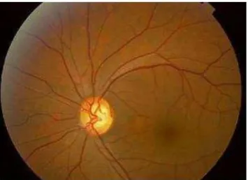
The normal fundus and the abnormal fundus images are given as input and shown in Figure 2.1 and 2.2.
K.GunaSeelan et al, International Journal of Computer Science and Mobile Applications, Vol.2 Issue. 3, March- 2014, pg. 66-74 ISSN: 2321-8363
©2014, IJCSMA All Rights Reserved, www.ijcsma.com 68
Figure 2.2Inputs Abnormal RGB Image
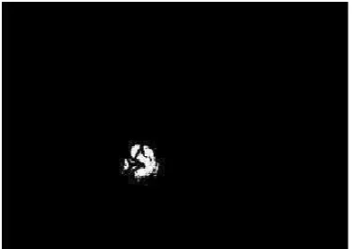
The result of normal image after thresholding is shown in Figure 2.3 and the result obtained from abnormal image is shown in Figure 2.4
Figure 2.3 Output Normal Binary Image
Figure 2.4 Output Abnormal Binary Image
K.GunaSeelan et al, International Journal of Computer Science and Mobile Applications, Vol.2 Issue. 3, March- 2014, pg. 66-74 ISSN: 2321-8363
©2014, IJCSMA All Rights Reserved, www.ijcsma.com 69
3 Iteration Method
This is a density based method. Initially the RGB image obtained from the fundus camera was converted to Gray-scale and then a window of arbitrary size was chosen and it was made to scan the entire retinal image. The algorithm works in such a way that, the number of pixels exceeding intensity value in the window was compared with a certain threshold value. When the density of pixels was greater than the threshold, it made the entire area under the window to be white. Instead, if the density of pixels was less than the threshold, it made the entire area under the window to be black. This was the first iteration. In the subsequent iterations, the window size was increased from the previous one and the output of first iteration was fed as input and the above steps were repeated again. The whole process was repeated for a finite number of times. Finally binary image was obtained with a white rectangle representing the location of the optic disk. This can be mapped on to the RGB image. Thus in this iterative manner the approximate localization of optic disk was done.
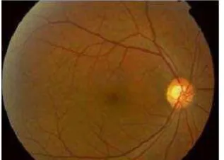
The input image is shown in Figure 3.5 and the gray image is shown in Figure2.6.The results of the iterations are shown in Figures 3.7 and 3.8.
Figure 3.5 Input Normal RGB Image
Figure 3.6 Gray Scale Image
K.GunaSeelan et al, International Journal of Computer Science and Mobile Applications, Vol.2 Issue. 3, March- 2014, pg. 66-74 ISSN: 2321-8363
©2014, IJCSMA All Rights Reserved, www.ijcsma.com 70
Figure 3.8 Second Iteration Output
In this method, the window moves sequentially. So a tiny part of the optic disk perhaps the edge may fall into a window such that the major part is the surrounding pixels of the optic disk. Since the entire area under the window is made black, the edges may get eroded and this affects the final result.
4 Clustering
This is a distance based mostly technique. The calculation of threshold is completed by easy mean estimation technique and multiplying the mean image by a scaling issue. A scaling issue of zero.85 is appropriate. the grey scale image is at first scanned element by element. for each element extraordinary the threshold a box of size (5 x 5) is made. This box is named a cluster. The x and y co- ordinates of the element is updated into 2 vectors row and column. ranging from the primary entry within the vectors a box with coordinate lying in a suitable level of distance is searched. To figure the distance basic mathematical formula
√(x2-x1)2+(y2-y1)2 --- (1)
is used. Once found the boxes square measure joined. The boxes square measure joined supported their location.
Say for instance, (x1, y1) be the center of mass of initial cluster and (x2, y2) be the center of mass of second cluster. when this the fundamental mathematical formula to evaluate the gap between 2 points is applied to find out the gap between the clusters. Keeping (x1, y1) because the reference the gap between this reference and also the center purpose of each other cluster is decided. The clusters having centroids inside a nominative distance from this reference center of mass purpose area unit combined. The northwest point of the reference cluster and also the Southeast point of the cluster that is nearer thereto area unit merged to create one cluster. Then afterwards these centroids area unit far from the list of centroids to be evaluated. This development is repeated for each alternative center of mass and also the clusters area unit regrouped. This technique is perennial on top of for certain time which provides bound candidate regions. For every candidate, range of pixels surpassing the threshold is found. If it's below a particular level determined by the scale of the candidate region the candidates area unit discarded. Finally we have a picture in which the candidate region utterly encloses the point although it should not precisely sq. it.
K.GunaSeelan et al, International Journal of Computer Science and Mobile Applications, Vol.2 Issue. 3, March- 2014, pg. 66-74 ISSN: 2321-8363
©2014, IJCSMA All Rights Reserved, www.ijcsma.com 71 pixels density. However in some pictures the exudates are as huge and thick as exudates. In such cases it's tough to seek out that of the candidate contains the point.
Figure 4.1 OUTPUT Of CLUSTERING
5 Principal component Analysis Between Clusters
PCA may be a statistical system. For every pixel a window is built around it with the pixel because the center .For every box PCA is applied and the one having minimum euclidean distance contains point. Our take a look at image size is 240 x 180.So the PCA method should be applied 43200 times. therefore it's terribly time intense and also the technique is not correct enough to attend farewell. Clustering does not show correct output for pictures with exudates. The advantage of the PCA and agglomeration can be combined. the most extract of this technique is that, the candidate regions are 1st determined by clustering the brightest pixels in application image. Principal element Analysis is then applied to these candidate regions. The candidate region having the smallest amount euclidean distance contains the optic disc. through the centre of the candidate region and centre of the point doesn't coincide, the region encloses the point.
Candidate region is decided by clustering technique. The agglomeration technique produces different range in candidate regions. But for applying PCA we want the candidate regions to be of mounted planned size. (40 x 40) in our case, so the candidates square measure resized. for each mounted size cluster we discover the brightest element and construct a forty x 40 box.
K.GunaSeelan et al, International Journal of Computer Science and Mobile Applications, Vol.2 Issue. 3, March- 2014, pg. 66-74 ISSN: 2321-8363
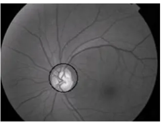
©2014, IJCSMA All Rights Reserved, www.ijcsma.com 72 Figure 5.1 guiding image
Figure 5.2 ABNORMAL INPUT IMAGE
Figure 5.3 OUTPUT USIN PCA METHOD
6.
Propagation During RADII
PCA between clusters produces output specified the point is confined during a square box of size (40 x 40). For fastened size boxes 1600 pixels square measure extracted considering it to be containing the point. however in several pictures the optic disc occupies solely around one thousand pixels. If any exudates lie at intervals proximity of the point then it may even be extracted. this could increase the chance of abnormal tissue layer being described traditional.
K.GunaSeelan et al, International Journal of Computer Science and Mobile Applications, Vol.2 Issue. 3, March- 2014, pg. 66-74 ISSN: 2321-8363
©2014, IJCSMA All Rights Reserved, www.ijcsma.com 73 The centre of the box containing optic disc is outlined by coordinates (A, B). normally to represent a circle in distinct house we have a tendency to use A+rcosθ, B+rsinθ. θ lies from zero to 360. The discretionary initial value of r is ten. so we have got ({A+10cos0, B+10sin0}, {A+10c0s1, B+10sin1}…{A+10cos360,B+10sin360}).. every of them representing some extent within the circumference of the circle. currently the primary purpose (corresponding to θ=0) on the circumference is taken. Keeping it because the centrepoint and a picture element is chosen higher than (A+(r+1)cosθ, B+(r+1)sinθ) and below(A+(r-1)cosθ, B+(r-1)sinθ) that. The distinction of picture element intensity worth between the higher purpose and center purpose and conjointly between lower purpose and center purpose is computed.
A threshold is about (5 in our case) and if the distinction value is larger than the brink create the middle point is formed black. This procedure is perennial till the distinction worth becomes larger than the threshold, whenever shifting the centre purpose upward on the radius by incrementing the initial r value .The final r worth is that the radius corresponding to that θ. this is often in dire straits all the points gift in the circumference of the circle i.e., for θ go from zero to 360. thus we have a tendency to get radius for all 360 degrees, then the mean radius is found. Our next step is to search out mean centre. this is often done by finding point of line connection circum points of supplementary angles for θ=0 to one hundred eighty. The mean of these x and y co-ordinates of the midpoints offers United States of America the mean centre. The circle of best work is drawn with mean centre because the centre and mean radius because the radius. As error margin may be intercalary to the mean radius, this ensures that the optic disk is totally
Figure 6.1 OUTPUT USING PROPAGATION THROUGH RADII
7 Conclusion
K.GunaSeelan et al, International Journal of Computer Science and Mobile Applications, Vol.2 Issue. 3, March- 2014, pg. 66-74 ISSN: 2321-8363
©2014, IJCSMA All Rights Reserved, www.ijcsma.com 74
References
[1] Li, H. and Chutatape, O.(2001) ‗Automatic location of Optic Disc in Retinal Images ‘, IEEE ICIP, pp.837- 840.
[2] Li, H. and Chutatape, O. (2003) ‗ A Model – based approach for Automated feature extraction in fundus images ‘, proceedings of the 9th IEEE International Conference on Computer Vision.
[3] Osareh, A, Mirmehdi, M, Thomas, B. and Markham, R, (2002)‗ Color Morphology and snakes for Optic Disc Localisation ‘, the 6th Medical Image Understanding and analysis Conference.
[4] Osareh, A, Mirmehdi, M, Thomas, B. and Markham, R, ‗ Comparison of Colour spaces for Optic Disc localization in Retinal images‘Pattern Recognition, 2002. Proceedings. 16th International Conference, volume1, pages:743-746.
[5] Li, H. and Chutatape, O.(2000) Fundus image features extraction ‘, Proceedings of the 22nd Annual International Conference of the IEEE Engineering in Medicine and Biology Society, Vol.4, pp.3071-3073.
[6] 6. Lupascu, C.A, D.Tegolo and L. Di Rosa,‘Automated Detection of Optic Disk localization in Retinal images‘, Computer-based medical System, 21st IEEE Int.Symp., 17- 19:17-22