Streamwise Feature Selection
Jing Zhou [email protected]
Electrical and Systems Engineering University of Pennsylvania
Philadelphia, PA 19104, USA
Dean P. Foster [email protected]
Robert A. Stine [email protected]
Statistics Department University of Pennsylvania Philadelphia, PA 19104, USA
Lyle H. Ungar [email protected]
Computer and Information Science University of Pennsylvania Philadelphia, PA 19104, USA
Editor: Isabelle Guyon
Abstract
In streamwise feature selection, new features are sequentially considered for addition to a predic-tive model. When the space of potential features is large, streamwise feature selection offers many advantages over traditional feature selection methods, which assume that all features are known in advance. Features can be generated dynamically, focusing the search for new features on promising subspaces, and overfitting can be controlled by dynamically adjusting the threshold for adding fea-tures to the model. In contrast to traditional forward feature selection algorithms such as stepwise regression in which at each step all possible features are evaluated and the best one is selected, streamwise feature selection only evaluates each feature once when it is generated. We describe information-investing andα-investing, two adaptive complexity penalty methods for streamwise feature selection which dynamically adjust the threshold on the error reduction required for adding a new feature. These two methods give false discovery rate style guarantees against overfitting. They differ from standard penalty methods such as AIC, BIC and RIC, which always drastically over- or under-fit in the limit of infinite numbers of non-predictive features. Empirical results show that streamwise regression is competitive with (on small data sets) and superior to (on large data sets) much more compute-intensive feature selection methods such as stepwise regression, and allows feature selection on problems with millions of potential features.
Keywords: classification, stepwise regression, multiple regression, feature selection, false discov-ery rate
1. Introduction
but expand the number of feature candidates while leaving the number of observations constant. For example, in a recent bankruptcy prediction study (Foster and Stine, 2004b), pairwise
interac-tions between the 365 original candidate features led to a set of over 67,000 resultant candidate
features, of which about 40 proved to be significant. The feature selection problem is to identify and include features from a candidate set with the goal of building a statistical model with minimal out-of-sample (test) error. As the set of potentially predictive features becomes ever larger, careful feature selection to avoid overfitting and to reduce computation time becomes ever more critical.
In this paper, we describe streamwise feature selection, a class of feature selection methods
in which features are considered sequentially for addition to a model, and either added to the
model or discarded, and two simple streamwise regression algorithms1, information-investing and
α-investing, that exploit the streamwise feature setting to produce simple, accurate models. Figure
1 gives the basic framework of streamwise feature selection. One starts with a fixed set of y values (for example, labels for observations), and each potential feature is sequentially tested for addition to a model. The threshold on the required benefit (for example, error or entropy reduction, or sta-tistical significance) for adding new features is dynamically adjusted in order to optimally control overfitting.
Streamwise regression should be contrasted with “batch” methods such as stepwise regression or support vector machines (SVMs). In stepwise regression, there is no order on the features; all features must be known in advance, since all features are evaluated at each iteration and the best feature is added to the model. Similarly, in SVMs or neural networks, all features must be known in advance. (Overfitting in these cases is usually avoided by regularization, which leaves all features in the model, but shrinks the weights towards zero.) In contrast, in streamwise regression, since potential features are tested one by one, they can be generated dynamically.
By modeling the candidate feature set as a dynamically generated stream, we can handle can-didate feature sets of unknown, or even infinite size, since not all potential features need to be generated and tested. Enabling selection from a set of features of unknown size is useful in many settings. For example, in statistical relational learning (Jensen and Getoor, 2003; Dzeroski et al., 2003; Dzeroski and Lavrac, 2001), an agent may search over the space of SQL queries to augment the base set of candidate features found in the tables of a relational database. The number of candi-date features generated by such a method is limited by the amount of CPU time available to run SQL queries. Generating 100,000 features can easily take 24 CPU hours (Popescul and Ungar, 2004), while millions of features may be irrelevant due to the large numbers of individual words in text. Another example occurs in the generation of transformations of features already included in the model (for example, pairwise or cubic interactions). When there are millions or billions of potential features, just generating the entire set of features (for example, cubic interactions or three-way table merges in SQL) is often intractable. Traditional regularization and feature selection settings assume that all features are pre-computed and presented to a learner before any feature selection begins. Streamwise regression does not.
Streamwise feature selection can be used with a wide variety of models where p-values or similar measures of feature significance are generated. We evaluate streamwise regression using
Input: A vector of y values (for example, labels), and a stream of features x.
{initialize}
model ={} //initially no features in model
i=1 // index of features
while CPU time used<max CPU time do
xi←get next feature()
{Is xia “good” feature?}
if fit of(xi, model)>threshold then
model←model∪xi // add xito the model
decrease threshold
else
increase threshold
end if i←i+1
end while
Figure 1: Algorithm: general framework of streamwise feature selection. The threshold on statis-tical significance of a future new feature (or the entropy reduction required for adding
the future new feature) is adjusted based on whether current feature was added. fit of(xi,
model) represents a score, indicating how much adding xi to the model improves the
model. Details are provided below.
linear and logistic regression (also known as maximum entropy modeling), where a large variety of selection criteria have been developed and tested. Although streamwise regression is designed for settings in which there is some prior knowledge about the structure of the space of potential features, and the feature set size is unknown, in order to compare it with stepwise regression, we apply streamwise regression in traditional feature selection settings, that is, those of fixed feature set size. In such settings, empirical evaluation shows that, as predicted by theory, for smaller feature sets such as occur in the UCI data sets, streamwise regression produces performance competitive to stepwise regression using traditional feature selection penalty criteria including AIC (Akaike, 1973), BIC (Schwartz, 1978), and RIC (Donoho and Johnstone, 1994; Foster and George, 1994). As feature set size becomes larger, streamwise regression offers significant computational savings and higher prediction accuracy.
The ability to do feature selection well encourages the use of different transformations of the original features. For sparse data, principal components analysis (PCA) or other feature extraction methods generate new features which are often predictive. Since the number of potentially useful principal components is low, it costs very little to generate a couple different projections of the data, and to place these at the head of the feature stream. Smaller feature sets should be put first. For example, first PCA components, then the original features, and then interaction terms. Results presented below confirm the efficiency of this approach.
Alternatively, features can be sorted so as to place potentially higher signal content features earlier in the feature stream, making it easier to discover the useful features. Different applications benefit from different sorting criteria. For example, sorting gene expression data on the variance of features sometimes helps (see Section 6.2). Often features come in different types (person, place, organization; noun, verb, adjective; car, boat, plane). A combination of domain knowledge and use of the different sizes of the feature sets can be used to provide a partial order on the features, and thus to take full advantage of streamwise feature selection. As described below, one can also dynamically re-order feature streams based on which features have been selected so far.
2. Traditional Feature Selection: A Brief Review
Traditional feature selection typically assumes a setting consisting of n observations and a fixed number m of candidate features. The goal is to select the feature subset that will ultimately lead
to the best performing predictive model. The size of the search space is therefore 2m, and
iden-tifying the best subset is NP-complete. Many commercial statistical packages offer variants of a greedy method, stepwise feature selection, an iterative procedure in which at each step all features are tested at each iteration, and the single best feature is selected and added to the model. Stepwise regression thus performs hill climbing in the space of feature subsets. Stepwise selection is termi-nated when either all candidate features have been added, or none of the remaining features lead to increased expected benefit according to some measure, such as a p-value threshold. We show below that an even greedier search, in which each feature is considered only once (rather than at every step) gives competitive performance. Variants of stepwise selection abound, including for-ward (adding features deemed helpful), backfor-ward (removing features no longer deemed helpful), and mixed methods (alternating between forward and backward). Our evaluation and discussion will assume a simple forward search.
There are many methods for assessing the benefit of adding a feature. Computer scientists tend to use cross-validation, where the training set is divided into several (say k) batches with equal
sizes. k−1 of the batches are used for training while the remainder batch is used for evaluation.
The training procedure is run k times so that the model is evaluated once on each of the batches and performance is averaged. The approach is computationally expensive, requiring k separate retraining steps for each evaluation. A second disadvantage is that when observations are scarce the method does not make good use of the observations. Finally, when many different models are being considered (for example, different combinations of features), there is a serious danger of overfitting when cross-validation is used. One, in effect, is selecting the model to fit the test set.
Penalized likelihood ratio methods (Bickel and Doksum, 2001) for feature selection are pre-ferred to cross-validation by many statisticians, as they do not require multiple re-trainings of the model and they have attractive theoretical properties. Penalized likelihood can be represented as:
score=−2 log(likelihood) +F×q
ben-Symbol Meaning
n Number of observations
m Number of candidate features
m∗ Number of beneficial features in the candidate feature set
q Number of features currently included in a model
Table 1: Symbols used throughout the paper and their definitions.
Name Nickname Penalty
Akaike information criterion AIC 2
Bayesian information criterion BIC log(n)
risk inflation criterion RIC 2 log(m)
Table 2: Different choices for the model complexity penalty F.
eficial2 or spurious features as those which, if added to the current model, would or would not reduce prediction error, respectively, on a hypothetical infinite large test data set. Note that under this definition of beneficial, if two features are perfectly correlated, the first one in the stream would be beneficial and the second one spurious, as it would not improve prediction accuracy. Also, if a prediction requires an exact XOR of two features, the raw features themselves could be spurious, even though the derived XOR-feature might be beneficial. We speak of the set of beneficial features
in a stream as those which would have improved the prediction accuracy of the model at the time
they were considered for addition if all prior beneficial features had been added.
Only features that decrease the score defined in Equation (1) are added to the model. In other words, the benefit of adding the feature to the model as measured by the likelihood ratio must surpass the penalty incurred by increasing the model complexity. We focus now on choice of F. Many different functions F have been used, defining different criteria for feature selection. The most widely used of these criteria are the Akaike information criterion (AIC), the Bayesian information criterion (BIC), and the risk inflation criterion (RIC). Table 2 summarizes the penalties F used in these methods.
For exposition we find it useful to compare the different choices of F as alternative coding schemes for use in a minimum description length (MDL) criterion framework (Rissanen, 1999). In MDL, both sender and receiver are assumed to know the feature matrix and the sender wants to send a coded version of a statistical model and the residual error given the model so that the receiver can construct the response values. Equation (1) can be viewed as the length of a message encoding a statistical model (the second term in Equation (1)) plus the residual error given that model (the first term in Equation (1)). To encode a statistical model, an encoding scheme must identify which features are selected for inclusion and encode the estimated coefficients of the included features. Using the fact that the log-likelihood of the data given a model gives the number of bits to code
the model residual error leads to the criteria for feature selection: accept a new feature xi only
if the change in log-likelihood from adding the feature is greater than the penalty F, that is, if
2 log(P(y|yˆxi))−2 log(P(y|yˆ−xi))>F where y is the response values, ˆyxi is the prediction when the
feature xiis added into the model, and ˆy−xi is the prediction when xiis not added. Different choices
for F correspond to different coding schemes for the model.
Better coding schemes encode the model more efficiently; they produce a more accurate
depic-tion of the model using fewer bits. AIC’s choice of F=2 corresponds to a version of MDL which
uses universal priors for the coefficient of a feature which is added into the model (Foster and Stine,
1999). BIC’s choice of F =log(n)employs more bits to encode the coefficient as the training set
size grows larger. Using BIC, each zero coefficient (feature not included in the model) is coded with
one bit, and each non-zero coefficient (feature included in the model) is coded with 1+12log(n)bits
(all logs are base 2). BIC is equivalent to an MDL criterion which uses spike-and-slab priors if the number of observations n is large enough (Stine, 2004).
However, neither AIC nor BIC are valid codes for mn. They thus are expected to perform
poorly as m grows larger than n, a situation common in streamwise regression settings. We confirm this theory through empirical investigation in Section 6.2.
RIC corresponds to a penalty of F =2 log(m)(Foster and George, 1994; George, 2000).
Al-though the criterion is motivated by a minimax argument, following Stine (2004) we can view RIC
as an encoding scheme where log(m)bits encode the index of which feature is added. Using RIC,
no bits are used to code the coefficients of the features that are added. This is based on the
assump-tion that m is large, so that the log(m)cost dominates the cost of specifying the coefficients. Such
an encoding is most efficient when we expect few of the m candidate features enter the model.
RIC can be problematic for streamwise feature selection since RIC requires that we know m in advance, which is often not the case (see Section 3). We are forced to guess a m, and when our guess
is inaccurate, the method may be too stringent or not stringent enough. By substituting F=2 log(m)
into Equation (1) and examining the resulting chi-squared hypothesis test, it can be shown that the
p-value required to reject the null hypothesis must be smaller than 0.m05. In other words, RIC may be
viewed as a Bonferroni p-value thresholding method. Bonferroni methods are known to be overly stringent (Benjamini and Hochberg, 1995), a problem exacerbated in streamwise feature selection applications when m should technically be chosen to be the largest number of features that might be examined. On the other hand, if m is picked to be a lower bound of the number of predictors that might be examined, then it is too small and there is increased risk that some feature will appear by chance to give significant performance improvement.
3. Interleaving Feature Generation and Testing
In streamwise feature selection, candidate features are sequentially presented to the modeling code for potential inclusion in the model. As each feature is presented, a decision is made using an adaptive penalty scheme as to whether or not to include the feature in the model. Each feature needs be examined at most once.
The “streamwise” view supports flexible ordering on the generation and testing of features. Features can be generated dynamically based on which features have already been added to the
model.3 Note that the theory provided below is independent of the feature generation scheme used.
All that is required is a method of generating features, and an estimation package which given a proposed feature for addition to the model returns a p-value for the corresponding coefficient or, more generally, the change in likelihood of the model resulting from adding the feature. One can also test the same feature more than once (as in stepwise regression), but we have not found significant benefit from doing multiple passes through the features.
New features can be generated in many ways. For example, in addition to the m original
fea-tures, m2pairwise interaction terms can be formed by multiplying all m2pairs of features together.
(Almost half of these features are, of course, redundant with the other half due to symmetry, and so
need not be generated and tested.) We refer to the interaction terms asgenerated features; they are
examples of a more general class of features formed from transformations of the original features (square root, log, etc.), or combinations of them including, for instance, PCA. Such strategies are frequently successful in obtaining better predictive models.
Rather than testing all possible interactions in an arbitrary order, it is generally better to initially test interactions of the features that have already been selected with themselves, then to test interac-tions of the selected features with the original features, and finally (if computer power permits) to test all interactions of the original features. This requires dynamic generation of the feature stream, since the first interaction terms can not be specified in advance, as they depend on which features have already been selected. (It can be the case, as in an XOR or parity problem, that interactions are significant when none of the individual component features are, but it still makes sense as a search strategy to try the smaller parts of the feature space first.)
Statistical relational learning (SRL) methods can easily generate millions of potentially predic-tive features as they “crawl” through a database or other relational structure and generate features by building increasingly complex compound relations or SQL queries (Popescul and Ungar, 2004). For example, when building a model to predict the journal in which an article will be published, potentially predictive features include the words in the target article itself, the words in the articles cited by the target article, the words in articles that cite articles written by the authors of the target article, and so forth.
Both stepwise regression and standard shrinkage methods require knowing all features in ad-vance, and are poorly suited for the feature sets generated by SRL. Since stepwise regression tests all features for inclusion at each iteration, it is computational infeasible on large data sets. Even if computer speed and memory were not an issue, control of overfitting using standard penalty meth-ods would fail. Some other strategy such as streamwise feature selection is required. Interleaving the generation of features with the assessment of model improvement allows the search over
tential features to be pruned to promising regions. A potentially intractable search thus becomes tractable.
In SRL, one searches further in those branches of a refinement graph where more component terms have proven predictive. In searching for interaction terms, one looks first for interactions or transformations of features which have proven significant. This saves the computation, and more importantly, avoids the need to take a complexity penalty for the many interaction terms which are never examined.
There are also simple ways to dynamically interleave multiple kinds of features, each of which is in its own stream. The main feature stream used in streamwise regression is dynamically constructed by taking the next feature from the sub stream which has had the highest success in having features accepted. If a previously successful stream goes long enough without having a feature selected, then other streams will be automatically tried. To assure that all streams are eventually tried, one can use a score for each stream defined as (number of features selected + a)/(number of features tried + b). The exact values of a and b do not matter, as long as both are positive. A single feature stream is used in this paper.
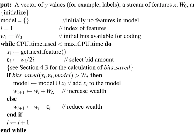
4. Streamwise Regression using Information-investing
Streamwise regression can be used either in an MDL setting (“information-investing”) or in a
sta-tistical setting using a t or F statistic (“α-investing”). We first present streamwise regression in an
information-investing setting. Information-investing (Ungar et al., 2005) is derived using a min-imum description length (MDL) approach (Stine, 2004). From a coding viewpoint, we wish to transmit a message to a receiver in order to let the receiver get the response values (y), assuming that the receiver knows x. In this sense, the score in Equation (1) is the description length required to code this message. The model is then chosen that minimizes the description length. If a feature is added to the model and reduces the description length, we call this reduction the bits saved. There-fore, bits saved is the decrease in the bits required to code the model error minus the increase in the bits required to code the model. The coding used to calculate bits saved is described in details in Section 4.3. If bits saved is larger than a threshold, we add the feature to the model. The algorithm
is shown in Figure 2. We set both W0and WΔ to 0.5 bit in all of the experiments presented in this
paper.
Information-investing allows us, for any valid coding, to have a false discovery rate (FDR) style bound, and thus to minimize the expected test error by adding as many features as possible subject to controlling the FDR bound (Zhou et al., 2005).
Streamwise regression with information-investing consists of three components:
• Wealth Updating: a method for adaptively adjusting the bits available to code the features
which will not be added to the model.
• Bid Selection: a method for determining how many bits,εi, one is willing to spend to code
the fact of not adding a feature xi. Asymptotically, it is also the probability of adding this
feature. We show below how bid selection can be done optimally by keeping track of the bits available to cover future overfitting (that is, the wealth).
• Feature Coding: a coding method for determining how many bits are required to code a
Input: A vector of y values (for example, labels), a stream of features x, W0, and WΔ.
{initialize}
model ={} //initially no features in model
i=1 // index of features
w1=W0 // initial bits available for coding
while CPU time used<max CPU time do
xi←get next feature()
εi←wi/2i // select bid amount
{see Section 4.3 for the calculation of bits saved}
if bits saved(xi,εi,model)>WΔthen
model←model∪xi// add xito the model
wi+1←wi+WΔ // increase wealth
else
wi+1←wi−εi // reduce wealth
end if i←i+1
end while
Figure 2: Algorithm: streamwise regression using information-investing.
4.1 Wealth Updating
The information-investing coding scheme is adjusted using the wealth, w, which represents the number of bits currently available for future overfitting. The wealth is “invested” in testing features.
Wealth starts at an initial value W0.
Each time a feature is added, it is (in expectation) likely to be a beneficial feature and lead to a decrease in the total description length, leaving more bits available to risk future overfitting. Thus,
wealth is increased by WΔ. By increasing wealth, we gain more feature selection power under the
FDR bound. Our algorithm guarantees that the sum of wealth (which is increased by WΔ) and total
description length (which is decreased by more than WΔ) is decreased. If a feature is not added to
the model,εbits is “invested” to code this fact and subtracted from wealth.
4.2 Bid Selection
The selection of εi as wi/2i gives the slowest possible decrease in wealth such that all wealth is
used; that is, so that as many features as possible are included in the model without systematically
overfitting.4
Theorem 1 Computingεi as proportional to wi/2i gives the slowest possible decrease in wealth
such that limi→∞wi=0.
Proof Defineδi=εi/wi to be the fraction of wealth invested at time i. If no features are added
to the model, wealth at time i is wi=Πi(1−δi). If we pass to the limit to generate w∞, we have
w∞=Πi(1−δi) =e∑log(1−δi)=e−∑δi+O(δ 2
i). Thus, w∞=0 iff∑δiis infinite.
Thus if we let δi go to zero faster than 1/i, say i−1−γ whereγ>0 then w∞>0 and we have
wealth that we never use.
4.3 Feature Coding
To code an added feature, we code both the fact that the feature is added and the value of its
esti-mated coefficient. Sinceεis the number of bits available to code the fact of not adding a feature, the
probability of not adding a feature should be e−εif the coding is optimal. Therefore, the probability
of adding a feature is 1−e−ε=1−(1−ε+O(ε2))≈ε, and the cost in bits of coding the fact the
feature is added is roughly−log(ε)bits. Different codings can be used for the feature’s estimated
coefficient. For example, BIC uses 12log(n)bits. In section 4.3.1, we present an optimal coding of
the estimated coefficients.
For now, for simplicity assume we use b bits to code each feature x’s estimated coefficient ˆβ
when x is added to the model. Adding x to the model reduces the model entropy by 12t2log(e)bits
where t is the t statistic associated with ˆβ, as defined above. Here, and below log()is log based 2;
the log(e)converts the t2to bits. Then,
bits saved=1
2t
2log(e)−(−log(ε) +b).
4.3.1 OPTIMALCODING OFCOEFFICIENTS ININFORMATION-INVESTING
A key question is what coding scheme to use to code the coefficient of a feature which is added to the model. We describe here an “optimal” coding scheme which can be used in the
information-investing criterion. The key idea is that coding an event with probability p requires log(p)bits. This
equivalence allows us to think in terms of distributions and thus to compute codes which handle
fractions of a bit. Our goal is to find a (legitimate) coding scheme which, given a “bid” ε, will
guarantee the highest probability of adding the feature to the model. We show below that given
any actual distribution ˜fβof the coefficients, we can produce a coding corresponding to a modified
distribution fβwhich produces a coding which uniformly dominates it.
Assume, for simplicity, that we increase the wealth by one bit when a feature xiwith coefficient
βiis added. Thus, when xiis added, we have
logp(xiis a beneficial feature)
p(xiis a spurious feature) >
1 bit,
that is, the log-likelihood decreases by more than one bit.
Let fβi be the distribution implied by the coding scheme for tβi if we add xi and f0(tβi) be the
normal distribution (the null model in which xi should not be added). The coding saves enough bits
to justify adding a feature whenever fβi(tβi)≥2 f0(tβi).This happens with probabilityαi≡p0({tβi:
fβi(tβi)≥2 f0(tβi)})under the null.αiis the area under the tails of the null distribution.
There is no reason to have fβi(tβi)2 f0(tβi)in the tails, since this would “waste” probability
112
1
1
t12 - t12
) ( 0ti
f β
0
i 0
2 ( )
( ) 1-2
( )
1
i i i
i
i
i
f t if t t
f t
f t otherwise
β β α
β β
β
α α
⎧ >
⎪ = ⎨
⎪ − ⎩
Figure 3: Optimal distribution fβ.
added. Using all of the remaining probability mass (or equivalently, making the coding “Kraft tight”) dictates the coding for the case when the feature is not likely to be added. The most efficient coding to use is thus:
fβ(tβi) =2 f0(tβi) if|tβi|>tαi
fβ(tβi) =1−2αi
1−αi f0(tβi) otherwise
and the corresponding cost in bits is:
log(fβ(tβi)/f0(tβi)) =log(2) =1 bit if|tβi|>tαi
log(fβ(tβi)/f0(tβi) =log(1−2αi
1−αi )≈ −αibits otherwise.
Figure 3 shows the distribution fβ(t(βi)), with the probability mass transferred away from the
center, where features are not added, out to the tails, where features are added.
The above equations are derived assuming that 1 bit is added to the wealth. It can be generalized
to add WΔbits to the wealth each time a feature is added to the model. Then, when a feature is added
to the model the probability of it being “beneficial” should be 2WΔ times that of it being “spurious”,
and all of the 2’s in the above equations are replaced with 2WΔ.
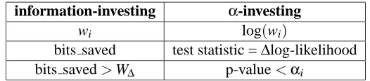
5. Streamwise Regression using Alpha-investing
One can define an alternate form of streamwise regression,α-investing (Zhou et al., 2005), which
is phrased in terms of p-values rather than information theory. The p-value associated with a t-statistic is the probability that a coefficient of the observed size could have been estimated by chance even though the true coefficient was zero (Larsen and Marx, 2001). Of the three components of
streamwise regression using information-investing, inα-investing, wealth updating is similar, bid
selection is identical, and feature coding is not required. The two different streamwise regression
algorithms are asymptotically identical (the wealth update ofαΔ−αiapproaches the update of WΔ
asαi becomes small), but differ slightly when the initial features in the stream are considered. The
relation between the two methods follows from the fact that coding an event with probability p
requires log(p)bits. Theα-investing algorithm is shown in Figure 4, and the equivalence between
α-investing and information-investing is shown in Table 3. Wealth updating is now done in terms
Input: A vector of y values (for example, labels), a stream of features x, W0, andαΔ.
{initialize}
model ={} //initially no features in model
i=1 // index of features
w1=W0 // initial prob. of false positives
while CPU time used<max CPU time do
xi←get next feature()
αi←wi/2i
{Is p-value of the new feature below threshold?}
if get p-value(xi,model)<αithen
model←model∪xi // add xito the model
wi+1←wi+αΔ−αi// increase wealth
else
wi+1←wi−αi // reduce wealth
end if i←i+1
end while
Figure 4: Algorithm: streamwise regression withα-investing.
information-investing α-investing wi log(wi)
bits saved test statistic =Δlog-likelihood
bits saved>WΔ p-value<αi
Table 3: The equivalence ofα-investing and information-investing.
α-investing controls the FDR bound by dynamically adjusting a threshold on the p-statistic
for a new feature to enter the model (Zhou et al., 2005). Similarly to the information-investing,
α-investing adds as many features as possible subject to the FDR bound giving the minimum
out-of-sample error.
The threshold, αi, corresponds to the probability of including a spurious feature at step i. It
is adjusted using the wealth, wi, which represents the current acceptable number of future false
positives. Wealth is increased when a feature is added to the model (presumably correctly, and hence permitting more future false positives without increasing the overall FDR). Wealth is decreased when a feature is not added to the model. In order to save enough wealth to add future features, bid selection is identical to the information-investing.
More precisely, a feature is added to the model if its p-value is greater thanα. The p-value is
computed by using the fact thatΔlog-likelihood is equivalent to a t-statistic. The idea ofα-investing
is to adaptively control the threshold for adding features so that when new (probably predictive)
features are added to the model, one “invests”αincreasing the wealth, raising the threshold, and
allowing a slightly higher future chance of incorrect inclusion of features. We increase wealth by
αΔ−αi. Note that whenαi is very small, this increase amount is roughly equivalent toαΔ. Each
two user-adjustable parameters,αΔand W0, which can be selected to control the FDR; we set both
of them to 0.5 in all of the experiments presented in this paper.
6. Experimental Evaluation
We compared streamwise feature selection usingα-investing against both streamwise and stepwise
feature selection (see Section 2) using the AIC, BIC and RIC penalties on a battery of synthetic and real data sets. After a set of features are selected from the real data sets, we applied logistic regression on this feature set selected, calculated the probability of observation labels, provided a cutoff/threshold of 0.5 to classify the response labels if label values are binary and get the prediction accuracies or balance errors. (Actually, different cutoffs could be used for different loss functions.) Information-investing gives extremely similar results, so we do not report them. We used R to implement our evaluation.
6.1 Evaluation on Synthetic Data
The base synthetic data set contains 100 observations each of 1,000 features, of which 4 are
pre-dictive. We generated the features independently from a normal distribution, N(0,1), with the true
model being the sum of four of the features (their coefficients are one’s)5plus noise, N(0,0.12). The
artificially simple structure of the data (the features are uncorrelated and have relatively strong sig-nal) allows us to easily see which feature selection methods are adding spurious features or failing to find features that should be in the model.
The results are presented in Table 4. As expected, AIC massively overfits, always putting in as many features as there are observations. BIC overfits severely, although less badly than AIC. RIC
gives performance comparable toα-investing. As one would also expect, if all of the beneficial
features in the model occur at the beginning of the stream,α-investing does better, giving the same
error as RIC, while if all of the beneficial features in the model are last,α-investing does (two times)
worse than RIC. In practice, if one is not taking advantage of known structure of the features, one can randomize the feature order to avoid such bad performance.
Stepwise regression gave noticeably better results than streamwise regression for this problem when the penalty is AIC or BIC. Using AIC and BIC still resulted in n features being added, but at least all of the beneficial features were found. Stepwise regression with RIC gave the same error of its streamwise counterpart. However, using standard code from R, the stepwise regression was
much slower than streamwise regression. Running stepwise regression on data sets with tens of
thousands of features, such as the ones presented in Table 5, was not possible.
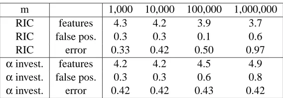
One might hope that adding more spurious features to the end of a feature stream would not
severely harm an algorithm’s performance.6 However, AIC and BIC, since their penalty is not a
function of m, will add even more spurious features (if they haven’t already added a feature for every observation!). RIC (Bonferroni) produces a harsher penalty as m gets large, adding fewer
and fewer features. As Table 5 and 6 show,α-investing is clearly the superior method in this case.
5. Similar results are also observed, if instead of using coefficients which are strictly 0 or 1, we use coefficients that are generated in either of the two cases: (a) most coefficients are zeros and several are from Gaussian distribution; (b) all coefficients are generated from t distribution with degree of freedom of two.
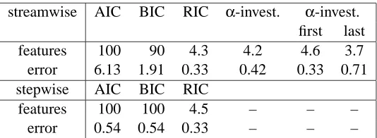
streamwise AIC BIC RIC α-invest. α-invest.
first last
features 100 90 4.3 4.2 4.6 3.7
error 6.13 1.91 0.33 0.42 0.33 0.71
stepwise AIC BIC RIC
features 100 100 4.5 – – –
error 0.54 0.54 0.33 – – –
Table 4: AIC and BIC overfit for mn. The number of features selected and the out-of-sample
error, averaged over 20 runs. n=100 observations, m=1,000 features, m∗=4 beneficial
features in data. Synthetic data: x∼N(0,1), y is linear in x with noiseσ2=0.1. Beneficial
features are randomly distributed in the feature set except the “first” and “last” cases. “first” and “last” denote the beneficial features being first or last in the feature stream.
m 1,000 10,000 100,000 1,000,000
RIC features 4.3 4.0 4.0 3.4
RIC false pos. 0.3 0.2 0.2 0.4
RIC error 0.33 0.42 0.50 0.97
α-invest. features 4.2 4.1 4.7 4.8
α-invest. false pos. 0.3 0.2 0.7 0.9
α-invest. error 0.42 0.42 0.43 0.45
Table 5: Effect of adding spurious features. The average number of features selected, false
posi-tives, and out-of-sample error (20 runs). m∗=4 beneficial features, randomly distributed
over the first 1,000 features. Otherwise the same model as Table 4.
Table 6 shows that when the number of potential features goes up to 1,000,000, RIC puts in one less beneficial feature, while streamwise regression puts the same four beneficial features plus a half of a spurious feature. Thus, streamwise regression is able to find the extra feature even when the feature is way out in the 1,000,000 features.
6.2 Evaluation on Real Data
Tables 7, 8, and 9 provide a summary of the characteristics of the real data sets that we used. All are for binary classification tasks. The six data sets in Table 7 were taken from the UCI repository. The seven data sets in Table 8 are bio-medical data, in which each feature represents a gene expression value for each observation (patient with cancer or healthy donor). For example, in aml data set, observations consist of patients with acute myeloid leukemia and patients with acute lymphoblastic leukemia. The classification task is to identify which patient has which cancer. ha and hung are private data sets and other gene expression data sets are available to the public (Li and Liu, 2002). The NIPS data sets are from the NIPS2003 workshop (Guyon, 2003).
m 1,000 10,000 100,000 1,000,000
RIC features 4.3 4.2 3.9 3.7
RIC false pos. 0.3 0.3 0.1 0.6
RIC error 0.33 0.42 0.50 0.97
αinvest. features 4.2 4.2 4.5 4.9
αinvest. false pos. 0.3 0.3 0.6 0.8
αinvest. error 0.42 0.42 0.43 0.42
Table 6: Effect of adding spurious features. The average number of features selected, false
posi-tives, and out-of-sample error (20 runs). m∗=4 beneficial features: when m=1,000, all
four beneficial features are randomly distributed; in the other three cases, there are three beneficial features randomly distributed over the first 1,000 features and another benefi-cial feature randomly distributed within the feature index ranges [1001, 10000], [10001,
100000], and [100001, 1000000] when m=10000, 100000, and 1000000 respectively.
Otherwise the same model as Table 4 and 5.
cleve internet ionosphere spect wdbc wpbc
features, m 13 1558 34 22 30 33
nominal features 7 1555 0 22 0 0
continuous features 6 3 34 0 30 33
observations, n 296 2359 351 267 569 194
baseline accuracy 54% 84% 64% 79% 63% 76%
Table 7: Description of the UCI data sets.
order, and averaged the five evaluation results. The baseline accuracy is the accuracy (on the whole data set) when predicting the majority class. The feature selection methods were tested on these data sets using ten-fold cross-validation.
On the UCI and gene expression data sets, experiments were done on two different feature sets. The first experiments used only the original feature set. The second interleaved feature selection and generation, initially testing PCA components and the original features, and then generating in-teraction terms between any of the features which had been selected and any of the original features. On the NIPS data sets, since our main concern is to compare against the challenge best models, we did only the second kind of experiment.
aml ha hung ctumor ocancer pcancer lcancer
features, m 7,129 19,200 19,200 2,000 15,154 12,600 12,533
observations, n 72 83 57 62 253 136 181
baseline accuracy 65% 71% 63% 65% 64% 57% 92%
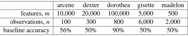
arcene dexter dorothea gisette madelon
features, m 10,000 20,000 100,000 5,000 500
observations, n 100 300 800 6,000 2,000
baseline accuracy 56% 50% 90% 50% 50%
Table 9: Description of the NIPS data sets. All features are nominal.
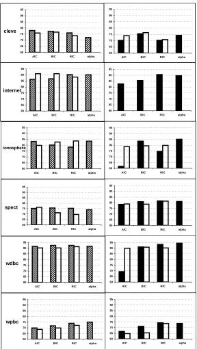
On UCI data sets (Figure 5)7 , when only the original feature set is used, paired two-sample
t-tests show thatα-investing has better performance than streamwise AIC and BIC only on two of
the six UCI data sets: the internet and wpbc data sets. On the other data sets, which have relatively few features, the less stringent penalties do as well as or better than streamwise regression. When
interaction terms and PCA components are included, α-investing gives better performance than
streamwise AIC on five data sets, than streamwise BIC on three data sets, and than streamwise RIC on two data sets. In general, when the feature set size is small, there is no significant difference in
the prediction accuracies betweenα-investing and the other penalties. When the feature set size is
larger (that is, when new features are generated)α-investing begins to show its superiority over the
other penalties.
On the UCI data sets (Figure 5), we also compared streamwise regression withα-investing8with
stepwise regression. Paired two-sample t-tests show that when the original feature set is used,α
-investing does not differ significantly from stepwise regression.α-investing has better performance
than stepwise regression in 5 cases, and worse performance in 3 cases. (Here a “case” is defined as
a comparison ofα-investing and stepwise regression under a penalty, that is, AIC or BIC or RIC,
on a data set.) However, when interaction terms and PCA components are included, α-investing
gives better performance than stepwise regression in 9 cases, and worse performance in none of the
cases. Thus, in our tests,α-investing is comparable to stepwise regression on the smaller data sets
and superior on the larger ones.
On the UCI data sets (Table 10), α-investing was also compared with support vector machines
(SVM), neural networks (NNET), and decision tree models (TREE). In all cases, standard packages
available with R were used9. No doubt these could be improved by fine tuning parameters and kernel
functions, but we were interested in seeing how well “out-of-the-box” methods could do. We did not tune any parameters in streamwise regression to particular problems either. Paired two-sample
t-tests show thatα-investing has better performance than NNET on 3 out of 6 data sets, and than
SVM and TREE on 2 out of 6 data sets. On the other data sets, streamwise regression doesn’t have
7. In Figure 5, a small training set size of 50 was selected to make sure the problems were difficult enough that the methods gave clearly different results. The right columns graphs differs from the left ones in that: (1) we generated PCA components from the original data sets and put them at the front of the feature sets; (2) after the PCA component “block” and the original feature “block”, there is an interaction term “block” in which the interaction terms are generated using the features selected from the first two feature blocks. This kind of feature stream was also used in the experiments on the other data sets. We were unable to compute the stepwise regression results on the internet data set using the software at hand when interaction terms and PCA components were included giving millions of potential features with thousands of observations. It is indicative of the difficulty of running stepwise regression on large data sets.
significant better or worse performance than NNET, SVM, or TREE. These tests shows that the performance of streamwise regression is at least comparable to those of SVM, NNET, and TREE.
On the gene expression data sets (Figure 6), when comparingα-investing with streamwise AIC,
streamwise BIC, and streamwise RIC, paired two-sample t-tests show that when the original features
are used, the performances ofα-investing and streamwise RIC don’t have significant difference on
any of the data sets. But when interaction terms and PCA components are included , RIC is often
too conservative to select even only one feature, whereasα-investing has stable performance and
the t-tests show thatα-investing has significant better prediction accuracies than streamwise RIC on
5 out of 7 data sets. Note that, regardless of whether or not interaction terms and PCA components
are included,α-investing always has much higher accuracy than streamwise AIC and BIC.
The standard errors (SE) of prediction accuracies in shuffles gave us sense of the approach
sensitivity to the feature order. When the original features are used, α-investing has a maximum
SE of four percent on pcancer and its other SEs are less than two percents in accuracy. When PCA
components and interaction terms are included, α-investing has a maximum SE of two percents
on ha and its other SEs are around or less than one percent. Streamwise RIC has similar SEs as
α-investing has, but streamwise AIC and BIC usually have one percent higher SEs thanα-investing
and streamwise RIC. We can see that the feature shuffles don’t change the performance much on most of gene expression data sets.
When PCA components and interaction terms are included and the original feature set is sorted in advance by feature value variance (one simple way of making use of the ordering in the stream),
the prediction accuracy ofα-investing on hung is increased from 79.3% to 86.7%; for the other gene
expression data, sorting gave no significant change.
Also note that, for streamwise AIC, BIC, and RIC, adding interaction terms and PCA
compo-nents often hurts. In contrast, the additional features have not much effect on α-investing. With
these additional features, the prediction accuracies ofα-investing are improved or kept the same on
4 out of 6 UCI data sets and 5 out of 7 gene data sets.
On the gene expression data sets (Figure 6), we also comparedα-investing with stepwise
re-gression. The results show that,α-investing is competitive with stepwise regression with the RIC
penalty. Stepwise regression with AIC or BIC penalties gives inferior performance.
On the NIPS data sets (Table 11), we compared α-investing against results reported on the
NIPS03 competition data set using other feature selection methods (Guyon et al., 2006). Table 11 shows the results we obtained, and compares them against the two methods which did best in the competition. These methods are BayesNN-DFT (Neal, 1996, 2001), which combines Bayesian neural networks and Bayesian clustering with a Dirichlet diffusion tree model and
greatest-hits-one (Gilad-Bachrach et al., 2004), which normalizes the data set, selects features using distance
information, and classifies them using a perceptron or SVM.
Different feature selection approaches such as those used in BayesNN-DFT can be contrasted based on their different levels of greediness. Screening methods or filters look at the relation
between y and each xi independently. In a typical screen, one computes how predictive each xi
(i=1...m) is of y (or how are they correlated), or the mutual information between them, and all features above a threshold are selected. In an extension of the simple screen, FBFS (Fleuret, 2004)
after one has been added.10 Streamwise and stepwise feature selection are one step less greedy,
sequentially adding features by computing I(y; xi|Model).
BayesNN-DFT uses a screening method to select features, followed by a sophisticated Bayesian
modeling method. Features were selected using the union of three univariate significance test-based screens (Neal and Zhang, 2003): correlation of class with the ranks of feature values, correlation of class with a binary form of the feature (zero/nonzero), and a runs test on the class labels reordered by increasing feature value. The threshold was selected by comparing each to the distribution found when permuting the class labels. This richer feature set of transformed variables could, of course, be used within the streamwise feature selection setting, or streamwise regression could be used to find an initial set of features to be provided to the Bayesian model.
greatest-hits-one applied margin based feature selection on data sets arcene and madelon, and
used a simple infogain ranker to select features on data sets dexter and dorothea. Assuming a fixed feature set size, a generalization error bound is proved for the margin based feature selection method (Gilad-Bachrach et al., 2004).
Table 11 shows that we mostly get comparable accuracy to the best-performing of the NIPS03 competition methods, while using a small fraction of the features. Many of the NIPS03 contestants got far worse performance, without finding small feature sets (NIPS’03, 2003). When SVM is used on the features selected by streamwise regression, the errors on arcene, gisette, and madelon are reduced further to 0.151, 0.021, 0.214 respectively. One could also apply more sophisticated methods, such as the Bayesian models which BayesNN-DFT used, to our selected features.
There is only one data set, madelon, where streamwise regression gives substantially higher error than the other methods. This may be partly due to the fact that madelon has substantially more observations than features, thus making streamwise regression (when not augmented with sophisticated feature generators) less competitive with more complex models. Madelon is also the only synthetic data set in the NIPS03 collection, and so its structure may benefit more from the richer models than typical real data.
7. Discussion: Statistical Feature Selection
Recent developments in statistical feature selection take into account the size of the feature space, but only allow for finite, fixed feature spaces, and do not support streamwise feature selection. The risk inflation criterion (RIC) produces a model that possesses a type of competitive predictive optimality. RIC chooses a set of features from the potential feature pool so that the loss of the
resulting model is within a factor of log(m)of the loss of the best such model. In essence, RIC
behaves like a Bonferroni rule (Foster and George, 1994). Each time a feature is considered, there is a chance that it will enter the model even if it is merely noise. In other words, the tested null hypothesis is that the proposed feature does not improve the prediction of the model. Doing a formal test generates a value for this null hypothesis. Suppose we only add this feature if its
p-value is less thanαj when we consider the jth feature. Then the Bonferroni rule keeps the chance
of adding even one extraneous feature to less than, say, 0.05 by constraining∑αj≤0.05.
Bonferroni methods like RIC are conservative, limiting the ability of a model to add features that
improve its predictive accuracy. The connection of RIC toα-spending rules leads to a more powerful
alternative. Anα-spending rule is a multiple comparison procedure that bounds its cumulative type
one error rate at a small level, say 5%. For example, suppose one has to test the m hypotheses
60 65 70 75 80 85 90 95
AIC BIC RIC alpha cleve 60 65 70 75 80 85 90 95
AIC BIC RIC alpha
internet 60 65 70 75 80 85 90 95
AIC BIC RIC alpha 60 65 70 75 80 85 90 95
AIC BIC RIC alpha
ionosphere 60 65 70 75 80 85 90 95
AIC BIC RIC alpha 60 65 70 75 80 85 90 95
AIC BIC RIC alpha
spect 60 65 70 75 80 85 90 95
AIC BIC RIC alpha 60 65 70 75 80 85 90 95
AIC BIC RIC alpha
wdbc 60 65 70 75 80 85 90 95
AIC BIC RIC alpha 60 65 70 75 80 85 90 95
AIC BIC RIC alpha
wpbc 60 65 70 75 80 85 90 95
AIC BIC RIC alpha 60 65 70 75 80 85 90 95
AIC BIC RIC alpha
cleve internet ionosphere
stream. (α-invest.) 84.3±1.8 (8.5) 96.5±0.3 (166) 91.4±1.8 (23)
SVM 82.0±2.0 93.4±0.6 92.2±1.7
NNET 70.3±4.5 84.2±0.9 91.7±1.9
TREE 76.0±3.3 96.5±0.5 86.7±1.8
spect wdbc wpbc
stream. (α-invest.) 82.2±2 (2) 95.1±0.6 (37) 77±3.4 (4.4)
SVM 81.5±2.4 96.3±0.8 76.5±4.9
NNET 78.9±2.2 68.8±4.5 75.0±5.0
TREE 81.1±1.9 94.2±0.9 74.0±3.0
Table 10: Comparison of streamwise regression and other methods on UCI Data. Average accuracy
using 10-fold cross validation. The number before±is the average accuracy; the
num-ber immediately after±is the standard deviation of the average accuracy. The number
in parentheses is the average number of features used by the streamwise regression, and these features includes PCA components, raw features, and interaction terms (see Foot-note 7 for the details of this kind of feature stream). SVM, NNET, and TREE use the whole raw feature set. Section 6.2 gives the results of paired two-sample t-tests.
arcene dexter dorothea gisette madelon
α-invest. error 0.176 0.067 0.090 0.037 0.295
α-invest. features 8 21 8 72 24
greatest-hits-one error 0.172 0.053 0.109 0.030 0.086
greatest-hits-one features 10,000 1,400 300 5,000 18
BayesNN-DFT error 0.133 0.039 0.085 0.013 0.072
BayesNN-DFT features 10,000 303 100,000 5,000 500
aml 50 55 60 65 70 75 80 85 90 95 100
AIC BIC RIC alpha
ha 50 55 60 65 70 75 80 85 90 95 100
AIC BIC RIC alpha
hung 50 55 60 65 70 75 80 85 90 95 100
AIC BIC RIC alpha
ctumor 50 55 60 65 70 75 80 85 90 95 100
AIC BIC RIC alpha
ocancer 50 55 60 65 70 75 80 85 90 95 100
AIC BIC RIC alpha
pcancer 50 55 60 65 70 75 80 85 90 95 100
AIC BIC RIC alpha
lcancer 50 55 60 65 70 75 80 85 90 95 100
AIC BIC RIC alpha
H1,H2,...,Hm. If we test the first using level α1, the second using level α2 and so forth with
∑jαj=0.05, then we have only a 5% chance of falsely rejecting one of the m hypotheses. If we
associate each hypothesis with the claim that a feature improves the predictive power of a regression, then we are back in the situation of a Bonferroni rule for feature selection. Bonferroni methods and
RIC simply fixαj=α/m for each test.
Alternative multiple comparison procedures control a different property. Rather than controlling
the cumulativeα(also known as the family wide error rate), they control the so-called false
discov-ery rate (Benjamini and Hochberg, 1995). Control of the FDR at 5% implies that at most 5% of the rejected hypotheses are false positives. In feature selection, this implies that of the included features, at most 5% degrade the accuracy of the model. The Benjamini-Hochberg method for controlling
the FDR suggests theα-investing rule used in streamwise regression, which keeps the FDR below
α: order the p-values of the independents tests of H1,H2,...,Hmso that p1≤p2≤ ···pm. Now find
the largest p-value for which pk≤α/(m−k)and reject all Hifor i≤k. Thus, if the smallest p-value
p1 ≤α/m, it is rejected. Rather than compare the second largest p-value to the RIC/Bonferroni
thresholdα/m, reject H2if p2≤2α/m. Our proposedα-investing rule adapts this approach to
eval-uate an infinite sequence of features. There have been many papers that looked at procedures of this sort for use in feature selection from an FDR perspective (Abramovich et al., 2000), an empirical Bayesian perspective (George and Foster, 2000; Johnstone and Silverman, 2004), an information theoretical perspective (Foster and Stine, 2004a), or simply a data mining perspective (Foster and Stine, 2004b). But all of these require knowing the entire list of possible features ahead of time.
Further, most of them assume that the features are orthogonal and hence tacitly assume that m<n.
Obviously, the Benjamini-Hochberg method fails as m gets large; it is a batch-oriented procedure.
The α-investing rule of streamwise regression controls a similar characteristic. Framed as a
multiple comparison procedure, the α-investing rule implies that, with high probability, no more
than α times the number of rejected tests are false positives. That is, the procedure controls a
difference rather than a rate. As a streamwise feature selector, if one has added, say, 20 features to the model, then with high probability (tending to 1 as the number of accepted features grows) no more than 5% (that is, one feature in the case of 20 features) are false positives.
8. Summary
A variety of machine learning algorithms have been developed over the years for online learning where observations are sequentially added. Algorithms such as the streamwise regression presented in this paper, which are online in the features being used are much less common. For some prob-lems, all features are known in advance, and a large fraction of them are predictive. In such cases, regularization or smoothing methods work well and streamwise feature selection does not make sense. For other problems, selecting a small number of features gives a much stronger model than trying to smooth across all potential features. (See JMLR (2003) and Guyon (2003) for a range of feature selection problems and approaches.) For example, in predicting what journal an article will
be published in, we find that roughly 10−20 of the 80,000 features we examine are selected
Empirical tests show that for the smaller UCI data sets where stepwise regression can be done, streamwise regression gives comparable results to stepwise regression or techniques such as deci-sion trees, neural networks, or SVMs. However, unlike stepwise regresdeci-sion, streamwise regresdeci-sion scales well to large feature sets, and unlike the AIC, BIC and RIC penalties or simpler variable screening methods which use univariate tests, streamwise regression with information-investing or
α-investing works well for all values of number of observations and number of potential features.
Key to this guarantee is controlling the FDR by adjusting the threshold on the information gain or p-value necessary for adding a feature to the model. Fortunately, given any software which incre-mentally considers features for addition and calculates their p-value or entropy reduction,
stream-wise regression using information-investing or α-investing is extremely easy to implement. For
linear and logistic regression, we have found that streamwise regression can easily handle millions of features.
The results presented here show that streamwise feature selection is highly competitive even when there is no prior knowledge about the structure of the feature space. Our expectation is that in real problems where we do know more about the different kinds of features that can be generated, streamwise regression will provide even greater benefit.
Acknowledgments
We thank Andrew Schein for his help in this work and Malik Yousef for supplying the data sets ha and hung.
References
F. Abramovich, Y. Benjamini, D. Donoho, and I. Johnstone. Adapting to unknown sparsity by controlling the false discovery rate. Technical Report 2000–19, Dept. of Statistics, Stanford University, Stanford, CA, 2000.
H. Akaike. Information theory and an extension of the maximum likelihood principle. In B. N. Petrov and F. Cs`aki, editors, 2nd International Symposium on Information Theory, pages 261– 281, Budapest, 1973. Akad. Ki`ado.
Y. Benjamini and Y. Hochberg. Controlling the false discovery rate: a practical and powerful ap-proach to multiple testing. Journal of the Royal Statistical Society, Series B(57):289–300, 1995.
P. Bickel and K. Doksum. Mathematical Statistics. Prentice Hall, 2001.
A. Blum and P. Langley. Selection of relevant features and examples in machine learning. Artificial
Intelligence, 97(1-2):245–271, 1997.
D. L. Donoho and I. M. Johnstone. Ideal spatial adaptation by wavelet shrinkage. Biometrika, 81: 425–455, 1994.
S. Dzeroski and N. Lavrac. Relational Data Mining. Springer-Verlag, 2001. ISBN 3540422897.
F. Fleuret. Fast binary feature selection with conditional mutual information. Journal of Machine
Learning Research, 5:1531–1555, 2004.
D. P. Foster and E. I. George. The risk inflation criterion for multiple regression. Annals of Statistics, 22:1947–1975, 1994.
D. P. Foster and R. A. Stine. Local asymptotic coding. IEEE Trans. on Info. Theory, 45:1289–1293, 1999.
D. P. Foster and R. A. Stine. Adaptive variable selection competes with Bayes experts. Submitted for publication, 2004a.
D. P. Foster and R. A. Stine. Variable selection in data mining: Building a predictive model for bankruptcy. Journal of the American Statistical Association (JASA), 2004b. 303-313.
E. I. George. The variable selection problem. Journal of the Amer. Statist. Assoc., 95:1304–1308, 2000.
E. I. George and D. P. Foster. Calibration and empirical bayes variable selection. Biometrika, 87: 731–747, 2000.
R. Gilad-Bachrach, A. Navot, and N. Tishby. Margin based feature selection - theory and algorithms. In Proc. 21’st ICML, 2004.
I. Guyon. Nips 2003 workshop on feature extraction and feature selection. 2003. URL
http://clopinet.com/isabelle/Projects/NIPS2003.
I. Guyon, S. Gunn, M. Nikravesh, and L. Zadeh. Feature Extraction, Foundations and Applications. Springer, 2006.
D. Jensen and L. Getoor. IJCAI Workshop on Learning Statistical Models from Relational Data. 2003.
JMLR. Special issue on variable selection. In Journal of Machine Learning Research (JMLR),
2003. URLhttp://jmlr.csail.mit.edu/.
I. M. Johnstone and B. W. Silverman. Needles and straw in haystacks: Empirical bayes estimates of possibly sparse sequences. Annals of Statistics, 32:1594–1649, 2004.
R. Kohavi and G. H. John. Wrappers for feature subset selection. Artificial Intelligence, 97(1-2): 273–324, 1997.
R. J. Larsen and M. L. Marx. An Introduction to Mathematical Statistics and Its Applications. Prentice Hall, 2001.
J. Li and H. Liu. Bio-medical data analysis. 2002. URLhttp://sdmc.lit.org.sg/GEDatasets.
R. M. Neal. Bayesian Learning for Neural Networks. Number 118 in Lecture Notes in Statistics. Springer-Verlag, 1996.
R. M. Neal and J. Zhang. Classification for high dimensional problems using bayesian neural networks and dirichlet diffusion trees. In NIPS 2003 workshop on feature extraction and feature
selection, 2003. URLhttp://www.cs.toronto.edu/ radford/slides.html.
NIPS’03. Challenge results. 2003. URLhttp://www.nipsfsc.ecs.soton.ac.uk/results.
A. Popescul and L. H. Ungar. Structural logistic regression for link analysis. In KDD Workshop on
Multi-Relational Data Mining, 2003.
A. Popescul and L. H. Ungar. Cluster-based concept invention for statistical relational learning. In
Proc. Conference Knowledge Discovery and Data Mining (KDD-2004), 2004.
J. Rissanen. Hypothesis selection and testing by the mdl principle. The Computer Journal, 42: 260–269, 1999.
G. Schwartz. Estimating the dimension of a model. The Annals of Statistics, 6(2):461–464, 1978.
R. A. Stine. Model selection using information theory and the mdl principle. Sociological Methods
Research, 33:230–260, 2004.
L. H. Ungar, J. Zhou, D. P. Foster, and R. A. Stine. Streaming feature selection using iic. In
AI&STAT’05, 2005.