Parallel Software for Training Large Scale Support Vector Machines
on Multiprocessor Systems
∗Luca Zanni [email protected]
Thomas Serafini [email protected]
Department of Mathematics
University of Modena and Reggio Emilia via Campi 213/B, Modena, 41100, Italy
Gaetano Zanghirati [email protected]
Department of Mathematics University of Ferrara
Scientific-Technological Campus, Block B via Saragat 1, Ferrara, 44100, Italy
Editors: Kristin P. Bennett and Emilio Parrado-Hern´andez
Abstract
Parallel software for solving the quadratic program arising in training support vector machines for classification problems is introduced. The software implements an iterative decomposition tech-nique and exploits both the storage and the computing resources available on multiprocessor sys-tems, by distributing the heaviest computational tasks of each decomposition iteration. Based on a wide range of recent theoretical advances, relevant decomposition issues, such as the quadratic sub-problem solution, the gradient updating, the working set selection, are systematically described and their careful combination to get an effective parallel tool is discussed. A comparison with state-of-the-art packages on benchmark problems demonstrates the good accuracy and the remarkable time saving achieved by the proposed software. Furthermore, challenging experiments on real-world data sets with millions training samples highlight how the software makes large scale standard nonlinear support vector machines effectively tractable on common multiprocessor systems. This feature is not shown by any of the available codes.
Keywords: support vector machines, large scale quadratic programs, decomposition techniques,
gradient projection methods, parallel computation
1. Introduction
Training support vector machines (SVM) for binary classification requires to solve the following convex quadratic programming (QP) problem (Vapnik, 1998; Cristianini and Shawe-Taylor, 2000)
min
F
(α) =12α
TGα−
∑
ni=1 αi
sub.to ∑ni=1yiαi=0,
0≤αi≤C, i=1, . . . ,n,
(1)
∗. This work was supported by the Italian Education, University and Research Ministry via the FIRB Projects
whose size n is equal to the number of examples in the given training set
D=
(xi,yi),i=1, . . . ,n, xi∈RM,yi∈ {−1,1} ,
and the entries of G are defined by
Gi j=yiyjK(xi,xj), i,j=1,2, . . . ,n,
where K :RM×RM→Rdenotes the kernel function. The main features of this problem are the density of the quadratic form and the special feasible region defined by box constraints and a sin-gle linear equality constraint. In many practical SVM applications, standard QP solvers based on the explicit storage of the Hessian matrix G may be very inefficient or, in the case of large data sets, even not applicable due to excessive memory requirements. For these reasons in recent years a lot of attention has been dedicated to this problem and several ad hoc strategies have been de-veloped, which are able to solve the problem with G out of memory. Among these strategies, the decomposition techniques have been the most investigated approaches and have given rise to the state-of-the-art software for the SVM QP problem. The idea behind the decomposition techniques consists in splitting the problem into a sequence of smaller QP subproblems, sized nspsay, that can be stored in the available memory and efficiently solved (Boser et al., 1992; Chang and Lin, 2001; Collobert and Bengio, 2001; Joachims, 1998; Osuna et al., 1997; Platt, 1998). At each decomposi-tion step, a subset of the variables, usually called working set, is optimized through the soludecomposi-tion of the subproblem in order to obtain a progress towards the minimum of the objective function
F
(α). Effective implementations of this simple idea involve important theoretical and practical issues. From the theoretical point of view, the policy for updating the working set plays a crucial role since it can guarantee the strict decrease of the objective function at each step (Hush and Scovel, 2003). The most used working set selections rely on the violations of the Karush-Kuhn-Tucker (KKT) first order optimality conditions. In case of working sets of minimal size, that is sized 2, a proper selec-tion via the maximal-violating pair principle (or related criteria) is sufficient to ensure asymptotic convergence of the decomposition scheme (Lin, 2002; Chen et al., 2005). For larger working sets, convergence proofs are available under a further condition which ensures that the distance between two successive approximations tends to zero (Lin, 2001a; Palagi and Sciandrone, 2005). Further-more, based on these working set selections and further assumptions, the linear convergence rate can be also proved (Lin, 2001b). For the practical efficiency of a decomposition technique, the fast convergence and the low computational cost per iteration seem the most important features. Unfor-tunately, these goals are conflicting since the strategies to improve the convergence rate (as the use of large working sets or the selections based on second order information) usually increase the cost per iteration. Examples of good trade-offs between the two goals are given by the most widely used decomposition packages: LIBSVM (Chang and Lin, 2001) and SVMlight(Joachims, 1998).The SVMlight algorithm uses a more general decomposition strategy, in the sense that it can also exploit working sets of size larger than 2. By updating more variables per iteration, such an approach is well suited for a faster convergence, but it introduces additional difficulties and costs. A generalized maximal-violating pair policy for the working set selection and a numerical solver for the inner QP subproblems are needed; furthermore, we must recall that the more variables are changed per iteration, the more expensive is the objective gradient updating. Even if SVMlightcan run with any working set size, numerical experiences show that it effectively faces the above diffi-culties only in case of small sized working sets (nsp=O(10)), where it often exhibits comparable performance with LIBSVM.
Following the SVMlight decomposition framework, another attempt to reach a good trade-off between convergence rate and cost per iteration was introduced by Zanghirati and Zanni (2003). This was the first approach suited for an effective implementation on multiprocessors systems. Unlike SVMlight, it is designed to manage medium-to-large sized working sets (nsp=O(102) or nsp=O(103)), that allow the scheme to converge in very few iterations, whose most expensive tasks (subproblem solving and gradient updating) can be easily and fruitfully distributed among the available processors. Of course, several issues must be addressed to achieve good performance, such as limiting the overhead for kernel evaluations and, also important, choosing a suitable inner QP solver. Zanghirati and Zanni (2003) obtained an efficient subproblem solution by a gradient projection-type method: it exploits the simple structure of the constraints, exhibits good conver-gence rate and is well suited for a parallel implementation. The promising results given by this parallel scheme can be now further improved thanks to some recent studies on both the gradient projection QP solvers (Serafini et al., 2005; Dai and Fletcher, 2006) and the selection rules for large sized working sets (Serafini and Zanni, 2005). On the basis of these studies a new parallel gradi-ent projection-based decomposition technique (PGPDT) is developed and implemgradi-ented in software available athttp://www.dm.unife/gpdt.
Other parallel approaches to SVMs have been recently proposed, by splitting the training data into subsets and distributing them among the processors. Some of these approaches, such as those by Collobert et al. (2002) and by Dong et al. (2003), do not aim to solve the problem (1) and then perform non-standard SVM training. Collobert et al. (2002) presented a mixture of multiple SVMs where, cyclically, single SVMs are trained on subsets of the training set and a neural network is used to assign samples to different subsets. Dong et al. (2003) used a block-diagonal approximation of the kernel matrix to derive independent SVMs and filter out the examples which are estimated to be non-support vectors; then a new serial SVM is trained on the collected support vectors. The idea to combine asynchronously-trained SVMs is revisited also by the cascade algorithm introduced by Graf et al. (2005). The support vectors given by the SVMs of a cascade layer are combined to form the training sets of the next layer. At the end, the global KKT conditions are checked and the process is eventually restarted from the beginning, re-inserting the computed support vectors in the training subsets of the first layer. The authors prove that this feedback loop allows the algorithm to converge to a solution of (1) and consequently to perform a standard training. Unfortunately, for all these approaches no parallel code is available yet.
with state-of-the-art serial packages and makes nonlinear SVMs tractable even on millions training samples.
The paper is organized as follows: Section 2 states the decomposition framework and describes its parallelization, Section 3 compares the PGPDT with SVMlightand LIBSVM on medium-to-large benchmark data sets and also faces some O(106)real-world problems, Section 4 draws the main conclusions and future developments.
2. The Decomposition Framework and its Parallelization
To describe in detail the decomposition technique implemented by PGPDT we need some basic notations. At each decomposition iteration, the indices of the variablesαi,i=1, . . . ,n, are split into the set
B
of basic variables, usually called the working set, and the setN
=1,2, . . . ,n \
B
of nonbasic variables. As a consequence, the kernel matrix G and the vectorsα= (α1, . . . ,αn)T and y= (y1, . . . ,yn)T can be arranged with respect toB
andN
as follows:G=
GB B GB N
GN B GN N
, α=
α
B
αN
, y=
yB
yN
.
Furthermore, we denote by nsp the size of the working set (nsp=#
B
) and by α∗ a solution of (1). Finally, suppose a distributed-memory multiprocessor system equipped with NPprocessors is available for solving the problem (1) and that each processor has a local copy of the training set.The decomposition strategy used by the PGPDT falls within the general scheme stated in Al-gorithm PDT. Here, we denote by the label “Distributed task” the steps where the NP processors cooperate to perform the required computation; in these steps communications and synchronization are needed. In the other steps, the processors asynchronously perform the same computations on the same input data to obtain a local copy of the expected output data.
It must be observed that algorithm PDT essentially follows the SVMlightdecomposition scheme proposed by Joachims (1998), but it allows to distribute among the available processors the sub-problem solution in step A2 and the gradient updating in step A3. Thus, two important implications can be remarked: from the theoretical viewpoint, the PDT algorithm satisfies the same convergence properties of the SVMlight algorithm, but, in practice, it requires new implementation strategies in order to effectively exploit the resources of a multiprocessor system. Here, we state the main con-vergence results of the PDT algorithm and we will describe in the next subsections how its steps have been implemented in the PGPDT software.
The convergence properties of the sequence{α(k)}generated by the PDT algorithm are mainly based on the special rule (4) for the working set selection. The rule was originally introduced by Joachims (1998) following an idea similar to the Zoutendijk’s feasible direction approach, to define basic variables that make possible a rapid decrease of the objective function. The asymptotic convergence of the decomposition schemes based on this working set selection was first proved by Lin (2001a) by relating the selection rule with the violation of the KKT conditions and by assuming the following strict block-wise convexity assumption on
F
(α):min
ALGORITHMPDT Parallel decomposition technique
A1. Initialization. Setα(1)=0 and let nspand ncbe two integer values such that n≥nsp≥nc>0, nceven. Choose nspindices for the working set
B
and set k=1.A2. QP subproblem solution. [Distributed task] Compute the solutionα(k+1)B of
min 1 2α
T
BGB BαB+
GB Nα(k)N −1B
T
αB
sub.to ∑i∈Byiαi=−∑i∈N yiα(k)i ,
0≤αi≤C, ∀i∈
B
,(2)
where 1B is the nsp-vector of all one; setα(k+1)=
α(k+1)
B
T
, α(k)N T T.
A3. Gradient updating. [Distributed task] Update the gradient
∇
F
(α(k+1)) =∇F
(α(k)) +
GB B
GN B
α(k+1)
B −α
(k)
B
(3)
and terminate ifα(k+1)satisfies the KKT conditions.
A4. Working set updating. Update
B
by the following selection rule:A4.1. Find the indices corresponding to the nonzero components of the solution of
min ∇
F
(α(k+1))Td sub.to yTd=0,di≥0 for i such thatα(k+1)i =0, di≤0 for i such thatα(k+1)i =C, −1≤di≤1,
#{di |di6=0} ≤nc.
(4)
Let ¯
B
be the set of these indices.where
J
is any subset of{1, . . . ,n}with #J
≤nspandλmin(GJ J)denotes the smallest eigenvalue ofGJ J. This condition is used to prove that there existsτ>0 such that
F
(α(k+1))≤F
(α(k))−τ2kα
(k+1)−α(k)k2 ∀k, (6) from which the important property limk→∞kα(k+1)−α(k)k=0 can be derived. Of course, the as-sumption (5) is satisfied when G is positive definite (for example, when the Gaussian kernel is used and all the training examples are distinct), but it may not hold in other instances of the problem (1). Convergence results that do not require the condition (5) are given by Lin (2002) and Palagi and Sciandrone (2005).
For the special case nsp=2, where the selection rule (4) gives only the two indices correspond-ing to the maximal violation of the KKT conditions (the maximal-violatcorrespond-ing pair), Lin (2002) has shown that the assumption (5) is not necessary to ensure the convergence.
For any working set size, Palagi and Sciandrone (2005) have shown that the condition (6) is ensured by solving at each iteration the following proximal point modification of the subproblem (2):
min 1 2α
T
BGB BαB+
GB Nα(k)N −1B
T
αB+τ
2kαB−α (k)
B k2
sub.to ∑i∈Byiαi=−∑i∈N yiα(k)i ,
0≤αi≤C, ∀i∈
B
.(7)
Unfortunately, this modification affects the behaviour of standard decomposition schemes in a way which is not completely understood yet. Our preliminary experiences suggest that sufficiently large values of τ can easily allow a better performance of the inner QP solvers, but those values often imply a dangerous decrease in the convergence rate of the decomposition technique. On the other hand, too small values forτdo not produce essential differences with respect to the schemes where the subproblem (2) is solved.
In the PGPDT software, besides the default setting which implements the standard PDT algo-rithm, two different ways to generate a sequence satisfying the condition (6) are available by user selection: (i) solving the subproblem (7) in place of (2) at each iteration or (ii) solving (7) only as emergency step, whenα(k+1)B obtained via (2) fails to satisfy (6). All the computational experiments of Section 3 are carried out with the default setting that generally yields the best performance. For what concerns the practical rule used in the PGPDT to stop the iterative procedure, the fulfilment of the KKT conditions within a prefixed tolerance is checked (with the equality constraint multiplier computed as suggested by Joachims, 1998). The default tolerance is 10−3, as it is usual in SVM packages, but different values can be selected by the user.
Before to describe the PGPDT implementation in detail, it must be recalled that this software is designed to be effective in case of sufficiently large nsp, i.e., when iterations with well parallelizable tasks are generated. For this reason, in the sequel the reader may assume nsp to be of medium-to-large size.
2.1 Parallel Gradient Projection Methods for the Subproblems
The inner QP subproblems (2) and (7) can fit into the following general form:
min
w∈Ω f(w) =
1 2w
where A∈Rnsp×nspis dense, symmetric and positive semidefinite, w,b∈Rnspand the feasible region
Ωis defined by
Ω={w∈Rnsp, ℓ≤w≤u, cTw=γ}, ℓ, u,c∈Rnsp, ℓ <u. (9)
We recall that the size nspis such that A can fit into the available memory.
Since subproblem (8) appears at each decomposition iteration, an effective inner solver becomes a crucial tool for the performance of a decomposition technique. The standard library QP solvers can be successfully applied only in the small size case (nsp=O(10)), since their computational cost easily degrades the performance of a decomposition technique based on medium-to-large nsp. For such kind of decomposition schemes, it is essential to design more efficient inner solvers able to exploit the special features of (8) and, for the PGPDT purposes, with the additional property to be easily parallelizable. To this end, the gradient projection methods are very appealing approaches (Bertsekas, 1999). They consist in a sequence of projections onto the feasible region, that are nonex-pensive operations in the case of the special constraints (9). In fact, the projection ontoΩ(denoted by PΩ(·)) can be performed in O(nsp)operations by efficient algorithms, like those by Pardalos and Kovoor (1990) and by Dai and Fletcher (2006). Furthermore, the single iteration core consists es-sentially in an nsp-dimensional matrix-vector product that is suited to be optimized (by exploiting the vector sparsity) and also to be parallelized. Thus, the simple and nonexpensive iteration moti-vates the interest for these approaches as possible alternative to standard solvers based on expensive factorizations (usually requiring O(n3sp)operations). A general parallel gradient projection scheme for (8) is depicted in Algorithm PGPM. As in the classical gradient projection methods, at each iteration a feasible descent direction d(k)is obtained by projecting ontoΩa point derived by taking a steepest descent step of length ρk from the current w(k). A linesearch procedure is then applied along the direction d(k)to decide the step sizeλkable to ensure the global convergence. The paral-lelization of this iterative scheme is simply obtained by a block row-wise distribution of A and by a parallel computation of the heaviest task of each iteration: the matrix-vector product Ad(k).
Concerning the convergence rate, that is the key element for the PGPM performance, the choices of both the steplengthρk and the linesearch parameter λk play a crucial role. Recent works have shown that appropriate selection rules for these parameters can significantly improve the typical slow convergence rate of the traditional gradient projection approaches (refer to Ruggiero and Zanni, 2000b, for the R-linear convergence of PGPM-like schemes). From the steplength viewpoint, very promising results are actually obtained with selection strategies based on the Barzilai-Borwein (BB) rules (Barzilai and Borwein, 1988):
ρBB1 k+1 =
d(k)Td(k)
d(k)TAd(k)
, ρBB2k+1= d
(k)TAd(k)
d(k)TA2d(k).
The importance of these rules has been observed in combination with both monotone and nonmono-tone linesearch strategies (Birgin et al., 2000; Dai and Fletcher, 2005; Ruggiero and Zanni, 2000a). In particular, for the SVM applications, the special BB steplength selections proposed by Serafini et al. (2005), for the monotone scheme, and by Dai and Fletcher (2006), for the nonmonotone method, seem very efficient.
ALGORITHMPGPM Parallel gradient projection method for step A2 of Algorithm PDT.
B1. Initialization.
[Data distribution] ∀p=1, . . . ,NP: allocate a row-wise slice Ap = (ai j)i∈Ip, j=1,...,nsp of A,
where
I
pis the subset of row indices belonging to processor p:I
p⊂ {1, . . . ,n}, NP[
p=1
I
p={1, . . . ,n},I
i∩I
j=/0 for i6= j.Furthermore, allocate local copies of all the other input data.
Initialize the parameters for the steplength selection rule and for the linesearch strategy.
Set w(0)∈Ω, 0<ρmin<ρmax, ρ0∈[ρmin,ρmax], k=0.
[Distributed task] ∀p=1, . . . ,NP: compute the local slice t(0)p =Apw(0) and send it to all the other processors; assemble a local copy of the full t(0)=Aw(0)vector.
Set g(0)=∇f(w(0)) =Aw(0)+b=t(0)+b .
B2. Projection.
Terminate if w(k)satisfies a stopping criterion; otherwise compute the descent direction
d(k)=PΩ w(k)−ρkg(k)−w(k).
B3. Matrix-vector product.
[Distributed task] ∀p=1, . . . ,NP: compute the local slice z(k)p =Apd(k)and send it to all the other processors; assemble a local copy of the full z(k)=Ad(k)vector.
B4. Linesearch.
Compute the linesearch stepλk and w(k+1)=w(k)+λkd(k).
B5. Update.
Compute
t(k+1)=Aw(k+1)=t(k)+λkAd(k)=t(k)+λkz(k),
g(k+1)=∇f(w(k+1)) =Aw(k+1)+b=t(k+1)+b,
and a new steplengthρk+1.
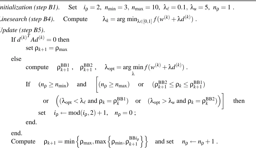
Initialization (step B1). Set iρ=2, nmin=3, nmax=10, λℓ=0.1, λu=5, nρ=1 .
Linesearch (step B4). Compute λk=arg minλ∈[0,1]f(w(k)+λd(k)). Update (step B5).
If d(k)TAd(k)=0 then setρk+1=ρmax
else
compute ρBB1k+1 , ρBB2k+1 , λopt=arg min
λ f(w
(k)+λd(k)).
If (nρ≥nmin) and
(nρ≥nmax) or (ρBB2k+1≤ρk≤ρBB1k+1) or
(λopt<λℓandρk=ρBB1k ) or (λopt>λuandρk=ρBB2k )
then
set iρ←mod(iρ,2) +1, nρ=0 ; end.
end.
Compute ρk+1=min
n
ρmax,max
n
ρmin,ρBBik+1ρoo and set nρ←nρ+1 .
Figure 1: linesearch and steplength rule for the GVPM method.
that was simply based on an alternation of the BB rules every three iterations. Furthermore, the numerical experiments reported by (Serafini et al., 2005) show that the GVPM is much more ef-ficient than the pr LOQO (Smola, 1997) and MINOS (Murtagh and Saunders, 1998) solvers, two softwares widely used within the machine learning community. GVPM steplength selection and linesearch are described in Figure 1.
The Dai-Fletcher scheme is based on the following steplength selection:
ρDF k+1=
∑m−1 i=0 s(k−i)
T s(k−i) ∑m−1
i=0 s(k−i) T
v(k−i)
, m≥1, (10)
where s(j)=w(j+1)−w(j)and v(j)=g(j+1)−g(j), (g(j)=∇f(w(j))), j=0,1, . . .. Observe that the case m=1 reduces to the standard BB ruleρBB1k+1. In order to frequently accept the full step w(k+1)=
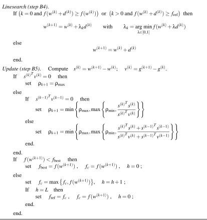
w(k)+d(k)generated with the above steplength, a special nonmonotone linesearch is used. Figure 2 describes the version of the Dai-Fletcher method corresponding to the parameters setting suggested by Zanni (2006) for the SVM applications. It may be observed that the linesearch parameterλk=
arg minλ∈[0,1] f(w(k)+λd(k))is used only if f(w(k)+d(k))≥ fref and not at each iteration, as in the GVPM. The steplength selection corresponds to the rule (10) with m=2 and, for what concerns the iteration cost, no significant additional tasks are required in comparison to the GVPM (g(k+1)is already available in step B5).
The PGPDT software can run the PGPM with either the GVPM or the Dai-Fletcher scheme, the latter being the default due to better experimental convergence rate (Zanni, 2006).
Initialization (step B1). Set L=2, fref=∞, fbest= fc= f(w(0)), h=0, k=0, s(k−1)=
v(k−1)=0 . Linesearch (step B4).
If k=0 and f(w(k)+d(k))≥ f(w(k))
or k>0 and f(w(k)+d(k))≥ fref
then
w(k+1)=w(k)+λkd(k) with λk=arg min
λ∈[0,1]
f(w(k)+λd(k))
else
w(k+1)=w(k)+d(k)
end.
Update (step B5). Compute s(k)=w(k+1)−w(k); v(k)=g(k+1)−g(k). If s(k)Tv(k)=0 then
set ρk+1=ρmax
else
If s(k−1)Tv(k−1)=0 then set ρk+1=min
(
ρmax,max
(
ρmin,s (k)Ts(k)
s(k)Tv(k)
))
else
set ρk+1=min
(
ρmax,max
(
ρmin,s
(k)Ts(k)+s(k−1)Ts(k−1) s(k)Tv(k)+s(k−1)Tv(k−1)
))
end.
end.
If f(w(k+1))< fbest then
set fbest=f(w(k+1)), fc= f(w(k+1)), h=0 ; else
set fc=maxfc,f(w(k+1)) , h=h+1 ; If h=L then
set fref= fc, fc= f(w(k+1)), h=0 ; end.
end.
Figure 2: linesearch and steplength rule for the Dai-Fletcher method.
for the decomposition technique: the fulfilment of the KKT conditions within a prefixed tolerance. In the PGPDT, the tolerance required to the inner solver depends on the quality of the outer it-erateα(k): in the first iterations the same tolerance as the decomposition scheme is used, while a progressively lower tolerance is imposed whenα(k)nearly satisfies the outer stopping criterion. In our experience, a more accurate inner solution just from the beginning doesn’t imply remarkable increase of the overall performance.
2.2 Parallel Gradient Updating
The gradient updating in step A3 is usually the most expensive task of a decomposition iteration. Since the matrix G is assumed to be out of memory, in order to obtain∇
F
(α(k+1))some entries of G need to be computed and, consequently, some kernel evaluations are involved that can be very expensive in case of large sized input space and not much sparse training examples. Thus, any strat-egy able to save kernel evaluations or to optimize their computation is crucial for minimizing the time consumption for updating the gradient. The updating formula (3) allows to get∇F
(α(k+1))by involving only the columns of G corresponding to the indices for which(α(k+1)i −α(k)i )6=0, i∈B
. Further improvements in the number of kernel evaluations can be obtained by introducing a caching strategy, consisting in using an area of the available memory to store some elements of G to avoid their recomputation in subsequent iterations. PGPDT fills the caching area with the columns of G involved in (3); when the cache is full, the current columns substitute those that have not been used for the largest number of iterations. This simple trick seems to well combine with the working set selection used in step A4, which forces some indices of the currentB
to remain in the new work-ing set (see the next section for more details), and remarkable reduction of the kernel evaluations are often observed. Nevertheless, the improvements implied by a caching strategy are obviously dependent on the size of the caching area. To this regard, the large amount of memory available on modern multiprocessor systems is an appealing resource for improving the performance of a de-composition technique. One of the innovative features of PGPDT is to implement a parallel gradient updating where both the matrix-vector multiplication and the caching strategy are distributed among the processors. This is done by asking each processor to perform a part of the column combinations required in (3) and to make available its local memory for caching the columns of G. In this way, the gradient updating benefits not only from a computations distribution, but also from a reduction of the kernel evaluations due to much larger caching areas. Of course, these features are not shared by standard decomposition packages, designed to exploit the resources of only one processor. The main steps of the above parallel updating procedure are summarized in Algorithm PGU.Concerning the reduction of the kernel evaluations, it is worth to recall that the entries of G stored in the caching area can be used also for GB B in step A2. Moreover, for the computation of
the linear term in (2), the equality
GB Nα
(k)
N −1B =∇
F
B(α(k))
−GB Bα(k)B
can avoid additional kernel evaluations by exploiting already computed quantities.
ALGORITHMPGU Parallel gradient updating in step A3 of Algorithm PDT
i) Denote by Wp, p=1,2, . . . ,NP, the caching area of the processor p and by Githe i-th column of G. Let
B
1=ni∈B
| α(k+1)i −α(k)i 6=0o
,
B
n=ni∈B
1 | Gi∈/Wp, p=1,2. . . ,NPo
,
B
c=B
1\B
n.Distribute among the processors the sets
B
c andB
n and denote byB
c,pandB
n,p the sets of indices assigned to processor p. Make the distribution in such a way thatB
c=SNi=1PB
c,i,B
c,i∩B
c,j=/0 for i6=j, ∀i∈B
c,p ⇒ Gi∈Wp,B
n=SNi=1PB
n,i,B
n,i∩B
n,j=/0 for i6= jand by trying to obtain a well balanced workload among the processors.
ii) ∀p=1,2, . . . ,NP: use the columns Gi∈Wp, i∈
B
c,p, to computerp=
GB Bc,p
GN Bc,p
α(k+1)
Bc,p −α
(k)
Bc,p
,
then compute the columns Gi, i∈
B
n,p, necessary to obtainrp←rp+
GB Bn,p
GN Bn,p
α(k+1)
Bn,p −α
(k)
Bn,p
and store in Wp as much as possible of these columns, eventually by substituting those less recently used.
iii) ∀p=1,2, . . . ,NP: send rpto all the other processors and assemble a local copy of
∇
F
(α(k+1)) =∇F
(α(k)) +NP
∑
i=1ALGORITHMSP1 Selection procedure for step A4.1 of algorithm PDT.
i) Sort the indices of the variables according to yi∇
F
(α(k+1))i in decreasing order and letI
≡(i1,i2, . . . ,in)T be the sorted list (i.e., yi1∇F
(α(k+1))
i1 ≥yi2∇
F
(α(k+1))
i2 ≥. . .≥
yin∇
F
(α(k+1)) in).
ii) Repeat the selection of a pair(it,ib)∈
I
×I
, with t<b, as follows:– moving down from the top of the sorted list, choose it∈
I
top(α(k+1)), – moving up from the bottom of the sorted list, choose ib∈I
bot(α(k+1)), until ncindices are selected or a pair with the above properties cannot be found.iii) Let ¯
B
be the set of the selected indices.and Gaussian. The interested reader is referred to the available code for more details on their prac-tical implementation. We end this section by remarking that, in case of linear kernel, the updating formula (3) can be simplified in
t=
∑
i∈B1
yixi
α(k+1) i −α
(k) i
,
B
1=n
i∈
B
| α(k+1)i −α(k)i 6=0o
,
∇
F
(α(k+1))j=∇F
(α(k))j+yjxTjt, j=1,2, . . . ,n, (11)and the importance of a caching strategy is generally negligible. Consequently, PGPDT faces linear SVMs without any caching strategy and performs the gradient updating by simply distributing the n tasks (11) among the processors.
2.3 Working Set Selection
In this section we describe how the working set updating in step A4 of the PDT algorithm is imple-mented within PGPDT. It consists in two phases: in the first phase at most ncindices are chosen for the new working set by solving the problem (4), while in the second phase at least nsp−ncentries are selected from the current
B
to complete the new working set. The selection procedure in step A4.1 was first introduced by Joachims (1998) and then rigorously justified by Lin (2001a). In short, by using the notationI
top(α)≡i|(αi<C and yi=−1)or(αi>0 and yi=1) ,
I
bot(α)≡j|(αj>0 and yj=−1)or(αj<C and yj=1) ,
this procedure can be stated as in Algorithm SP1.
It is interesting to recall how this selection procedure is related to the violation of the first order optimality conditions. For the convex problem (1) the KKT conditions can also be written as
a feasibleα∗is optimal ⇐⇒ max i∈Itop(α∗)
yi∇
F
(α∗)i ≤ min j∈Ibot(α∗)ALGORITHMSP2 Selection procedure for step A4.2 of algorithm PDT.
i) Let ¯
B
be the set of indices selected in step A4.1.ii) Fill ¯
B
up to nspentries by adding the most recent indices† j∈B
satisfying 0<α(k+1)j <C; if these indices are not enough, then add the most recent indices j∈B
such thatα(k+1)j =0and, eventually, the most recent indices j∈
B
satisfyingα(k+1)j =C.iii) Set nc=min{nc,max{10,J,nnew}}, where J is the largest even integer such that J≤ nsp
10 and nnewis the largest even integer such that nnew≤#{j, j∈
B
¯ \B
};set
B
=B
¯, k←k+1 and go to step A2.†We mean the indices that are in the working setBsince the lowest number of consecutive iterations.
It means that, given a non-optimal feasibleα, there exists at least a pair(i,j)∈
I
top(α)×I
bot(α)satisfying
yi∇
F
(α)i>yj∇F
(α)j .Following Keerthi and Gilbert (2002), these pairs are called KKT-violating pairs and, from this point of view, the above selection procedure chooses indices(i,j)∈
I
top(α(k+1))×I
bot(α(k+1))by giving priority to those pairs which most violate the optimality conditions. In particular, at each iteration the maximal-violating pair is included in the working set: this property is crucial for the asymptotic convergence of a decomposition technique.From the practical viewpoint, the indices selected via problem (4) identify steepest-like feasible descent directions: this is aimed to get a quick decrease of the objective function
F
(α). Never-theless, for fast convergence, both nc and the updating phase in step A4.2 have a key relevance. In fact, as it is experimentally shown by Serafini and Zanni (2005), values of nc equal or close to nspoften yield a dangerous zigzagging phenomenon (i.e., some variables enter and leave the work-ing set many times), which can heavily degrade the convergence rate especially for large nsp. This drawback suggests to set nc sufficiently smaller than nspand then it opens the problem of how to select the remaining indices to fill up the new working set. The studies available in literature on this topic (see Hsu and Lin, 2002; Serafini and Zanni, 2005; Zanghirati and Zanni, 2003, and also the SVMlight code) suggest that an efficient approach consists in selecting these indices from the current working set. We recall in Algorithm SP2 the filling strategy recently proposed in (Serafini and Zanni, 2005) and used by the PGPDT software.nc. The reduction takes place only if ncis larger than an empirical threshold and it is controlled via the number of those new indices selected in step A4.1 that do not belong to the current working set.
3. Computational Experiments
The aim of this computational study is to analyse the PGPDT performance. To this end, it is also worth to show that the serial version of the proposed software (called GPDT) can train SVMs with effectiveness comparable to that of the state-of-the-art softwares LIBSVM (ver. 2.8) and SVMlight (ver. 6.01). Since there are no other parallel software currently available for comparison, the PGPDT will be evaluated in terms of scaling properties with respect to the serial packages.
Our implementation is an object oriented C++code and its parallel version uses standard MPI communication routines (Message Passing Interface Forum, 1995), hence it is easily portable on many multiprocessor systems. Most of the experiments are carried out on an IBM SP5, which is an IBM SP Cluster 1600 equipped with 64 nodes p5-575 interconnected by a high performance switch (HPS). Each node owns 8 IBM SMP Power5 processors at 1.9GHz and 16GB of RAM (2GB per CPU). The serial packages run on this computer by exploiting only a single CPU. PGPDT has been tested also on different parallel architectures and, for completeness, we report the results obtained on a system where less memory than in the IBM SP5 is available for each CPU: the IBM CLX/1024 Linux Cluster, that owns 512 nodes equipped with two Intel Xeon processors at 3.0GHz and 1GB of RAM per CPU. Both the systems are available at the CINECA Supercomputing center (Bologna, Italy,http://www.cineca.it).
The considered softwares are compared on several medium, large and very large test problems generated from well known benchmark data sets, described in the next subsection.
3.1 Test Problems
We trained Gaussian and polynomial SVMs with kernel functions K(xi,xj) =exp −kxi−xjk2/(2σ2)
and K(xi,xj) = s(xiTxj) +1
d
, respectively1.
In what follows we give some details on the databases used for the generation of the training sets, as well as on the SVM parameters we have chosen. Error rates are given as the percentage of misclassifications.
The UCI Adult data set (athttp://www.research.microsoft.com/∼jplatt/smo.html) al-lows to train an SVM to predict whether a household has an income greater than $50000. The inputs are 123-dimensional binary sparse vectors with sparsity level≈89%. We use the largest version of the data set, sized 32561. We train a Gaussian SVM with training parameters chosen accord-ingly to the database technical documentation, i.e., C=1 andσ=√10, that are indicated as those maximizing the performance on a (unavailable) validation set.
The Web data set (available athttp://www.research.microsoft.com/∼jplatt/smo.html) concerns a web page classification problem with a binary representation based on 300 keyword features. On average, the sparsity level of the examples is about 96%. We use the largest version of the data set, sized 49749. We train a Gaussian SVM with the parameters suggested in the data set documentation: C=5 and σ=√10. As before, these values are claimed to give the best performance on a (unavailable) validation set.
The MNIST database of handwritten digits (http://yann.lecun.com/exdb/mnist) contains 784-dimensional nonbinary sparse vectors; the data set size is 60000 and the data sparsity is ≈ 81%. The provided test set is sized 10000. We train two SVM classifiers for the digit “8” with the following parameters: C=10,σ=1800 for the Gaussian kernel and C=3000, d=4, s=3·10−9 for the polynomial kernel. This setting gives the following error rates on the test set: 0.55% for the Gaussian kernel and 0.60% for the polynomial kernel.
The Forest Cover Type data set2has 581012 samples with 54 attributes, distributed in 8 classes. The average sparsity level of the samples is about 78%. We train some SVM classifiers for separat-ing class 2 from the other classes. The trainseparat-ing sets, sized up to 300000, are generated by randomly sampling the data set. We use a Gaussian kernel withσ2=2.5·104, C=10. For the largest training set the error rate is about 3.6% on the test set given by the remaining 281012 examples.
The KDDCUP-99 Intrusion Detection data set3consists in binary TCP dump data from seven weeks of network traffic. Each original pattern has 34 continuous features and 7 symbolic fea-tures. As suggested by Tsang et al. (2005), we normalize each continuous feature to the range[0,1]
and transform each symbolic feature to multiple binary features. In this way, the inputs are 122-dimensional sparse vectors with sparsity level≈90%. We work with the whole training set sized 4898431 and with some smaller subsets obtained by randomly sampling the original database. We use a Gaussian kernel with parametersσ2= (1.2)−1, C=2. This choice yields error rates of about 7% on the test set of 311029 examples available in the database.
3.2 Serial Behaviour
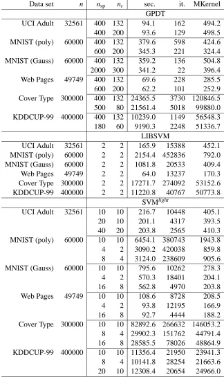
In the first experiments set, we analyse the behaviour of the serial code on the test problems just described. In Table 1 we report the time in seconds (sec.), the decomposition iteration count (it.) and the number of kernel evaluations in millions (MKernel) required for each one of the considered SVM training packages. The values we use for the working set parameters nsp and nc are also reported: as mentioned, the LIBSVM software works only with nsp=nc=2, whilst both SVMlight and GPDT accept larger values. For these two softwares, meaningful ranges of parameters were explored: we report the results corresponding to the pairs that gave the best training time and to the default setting (nsp=nc=10 for SVMlight, nsp=400, nc=⌊nsp/3⌋=132 for GPDT). SVMlightis run with several values of nspin the range[2,80]with both its inner solvers: the Hildreth-D’Esopo and the pr LOQO. The best training time is obtained by using the Hildreth-D’Esopo solver with nsp small and nc=nsp/2, generally observing a significant performance decrease for nsp>40.
We run the codes assigning to the caching area 512MB for the MNIST test problems and 768MB in the other cases; the default threshold ε=10−3 for the termination criterion is used, except for the two largest Cover Type and KDDCUP-99 test problems, where the stopping toleranceεis set to 10−2. All the other parameters are assigned default values. This means that both LIBSVM and SVMlightbenefit from the shrinking (Joachims, 1998) strategy that is not implemented in the current release of GPDT.
Table 1 well emphasizes the different approach of the three softwares. In particular we see how GPDT, by exploiting large working sets, converges in far less iterations than the other softwares, but its iterations are much heavier. Looking at the computational time, GPDT seems to be very competitive with respect to both LIBSVM and SVMlight. Furthermore, the kernel column highlights
Data set n nsp nc sec. it. MKernel GPDT
UCI Adult 32561 400 132 94.1 162 494.2 400 200 93.6 129 498.5 MNIST (poly) 60000 400 132 379.6 598 424.6 600 200 345.3 221 324.4 MNIST (Gauss) 60000 400 132 359.2 136 504.8 2000 300 341.2 22 396.4 Web Pages 49749 400 132 69.6 228 285.5 600 200 62.2 101 252.9 Cover Type 300000 400 132 24365.5 3730 120846.5 500 80 21561.4 5018 99880.0 KDDCUP-99 400000 400 132 10239.0 1149 56548.3 180 60 9190.3 2248 51336.7
LIBSVM
UCI Adult 32561 2 2 165.9 15388 452.1 MNIST (poly) 60000 2 2 2154.4 452836 792.0 MNIST (Gauss) 60000 2 2 1081.8 20533 409.4 Web Pages 49749 2 2 64.0 13237 170.3 Cover Type 300000 2 2 17271.7 274092 53152.6 KDDCUP-99 400000 2 2 11220.8 40767 50773.8
SVMlight
UCI Adult 32561 10 10 216.7 10448 405.1 20 10 201.1 4317 393.5 40 20 203.8 2565 410.3 MNIST (poly) 60000 10 10 6454.1 380743 1943.8 4 2 3090.2 420038 859.8 8 4 3124.0 238609 905.6 MNIST (Gauss) 60000 10 10 795.6 10262 278.3 4 2 570.3 18401 204.1 16 8 562.8 4970 203.8 Web Pages 49749 10 10 108.6 8728 208.5 4 2 93.8 12195 166.9 16 8 92.7 4444 188.2 Cover Type 300000 10 10 82892.6 266632 146053.2 8 4 29902.3 151762 44791.4 16 8 28585.5 78026 48864.9 KDDCUP-99 400000 10 10 11356.4 21950 23941.3 8 4 10141.8 28254 21663.6 20 10 12308.4 20654 24966.0
Solver SV BSV
F
opt b test error MNIST (poly) test problemGPDT 2712 640 −2555033.8 3.54283 0.63% LIBSVM 2715 640 −2555033.6 3.54231 0.63% SVMlight 2714 640 −2555033.0 3.54213 0.62%
Cover Type test problem
GPDT 50853 32683 −299399.7 0.22083 3.62% LIBSVM 51131 32573 −299396.0 0.22110 3.63% SVMlight 51326 32511 −299393.9 0.22149 3.62%
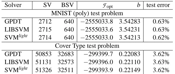
Table 2: accuracy of the serial solvers.
how GPDT benefits from a good optimization of the execution time for the kernel computation: compare, for instance, the results for the MNIST Gaussian test, where the kernel evaluations are very expensive. Here, in front of a number of kernel evaluations similar to LIBSVM and larger than SVMlight, a significant lower training time is exhibited. The same consideration holds true for the MNIST polynomial test; however in this case the good GPDT performance is also due to a lower number of kernel evaluations.
The next experiments are intended to underline how the good training time given by GPDT is accompanied by scaling and accuracy properties very similar to the other packages. From the accuracy viewpoint, this is shown for two of the considered test problems by reporting in Table 2 the number of support vectors (SV) and bound support vectors (BSV), the computed optimal value
F
optof the objective function, the bias b of the separating surface expression4(Cristianini and Shawe-Taylor, 2000) and the error rate on the test set.For what concerns the scaling, Figure 3a shows, for the Cover Type test problem (the worst case for GPDT), the training time with respect to the problem size. All the packages exhibit almost the same dependence that, for this particular data set, seems between quadratic and cubic with respect to the number of examples. For completeness, the number of support vectors of these test problems is also reported in Figure 3b.
3.3 Parallel Behaviour
The second experiments set concerns with the behaviour of PGPDT. We evaluate PGPDT on the previous four largest problems and some very large problems sized O(106) derived from the KDDCUP-99 data set.
3.3.1 LARGETESTPROBLEMS
For a meaningful comparison against the serial version, PGPDT is run on the MNIST, Cover Type and KDDCUP-99 (n=400000) test problems with the same nsp, nc andε parameters as in the previous experiments; furthermore, the same amount of caching area (768MB) is now allocated on each CPU of the IBM SP5. Default values are assigned to the other parameters.
4. The support vectors are those samples in the training set corresponding toα∗i >0; the samples withα∗i =C are
18.75 37.5 75 150 220 300 101
102 103 104 105
Number of training examples ( × 103 )
Time (sec.)
GPDT LIBSVM SVMlight
(a) dependence on n.
18.75 0 37.5 75 150 220 300 10
20 30 40 50 60
Number of training examples ( × 103 )
Number of SV (
×
10
3 )
GPDT LIBSVM SVMlight
(b) number of support vectors.
Figure 3: scaling of the serial solvers on test problems from the Cover Type data set.
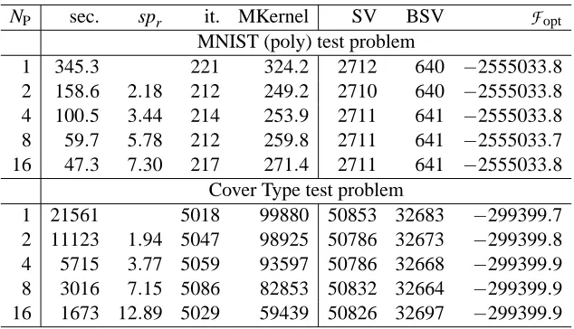
NP sec. spr it. MKernel SV BSV
F
opt MNIST (poly) test problem1 345.3 221 324.2 2712 640 −2555033.8 2 158.6 2.18 212 249.2 2710 640 −2555033.8 4 100.5 3.44 214 253.9 2711 641 −2555033.8 8 59.7 5.78 212 259.8 2711 641 −2555033.7 16 47.3 7.30 217 271.4 2711 641 −2555033.8
Cover Type test problem
1 21561 5018 99880 50853 32683 −299399.7 2 11123 1.94 5047 98925 50786 32673 −299399.8 4 5715 3.77 5059 93597 50786 32668 −299399.9 8 3016 7.15 5086 82853 50832 32664 −299399.9 16 1673 12.89 5029 59439 50826 32697 −299399.9
Table 3: PGPDT scaling on the IBM SP5 system.
Table 3 and Figure 4 summarize the results obtained by running PGPDT on different numbers of processors. We evaluate the parallel performance by the relative speedup, defined as spr=
Tserial/Tparallel, where Tserialis the training time spent on a single processor, while Tparalleldenotes the training time on NPprocessors.
bene-1 2 4 8 16 0 100 200 300 400 Time (sec.)
Number of processors
2 4 8 16 Relative speedup Linear speedup Time (sec) Rel. speedup
(a) MNIST (Gauss) test problem.
1 2 4 8 16
0 2000 4000 6000 8000 10000 Time (sec.)
Number of processors
2 4 8 16 Relative speedup Linear speedup Time (sec) Rel. speedup
(b) KDDCUP-99 (n=400000) test problem.
1 2 4 8 16
0 50 100 150 200 250 300 350 Time (sec.)
Number of processors
2 4 8 16 Relative speedup Linear speedup Time (sec) Rel. speedup
(c) MNIST (poly) test problem.
1 2 4 8 16
0 5000 10000 15000 20000 25000 Time (sec.)
Number of processors
2 4 8 16 Relative speedup Linear speedup Time (sec.) Rel. speedup
(d) Cover Type test problem.
Figure 4: PGPDT scaling on the IBM SP5 system.
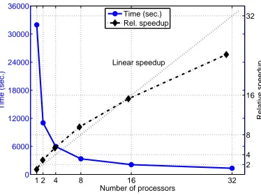
fits due to the parallel caching strategy are not sufficient to ensure optimal speedups. For instance, sometimes the nspvalues that give satisfactory serial performance are not suited for good PGPDT scaling. This is the case of the KDDCUP-99 test problem (Figure 4b), where the small working sets sized nsp=180 imply many decomposition iterations and consequently the fixed costs of the non-distributed tasks (working set selection and stopping rule) become very heavy. Another exam-ple is provided by the MNIST (polynomial) test problem (Figure 4c): here the subproblem solution is a dominant task in comparison to the gradient updating and the suboptimal scaling of the PGPM solver on 16 processors leads to poor speedups. However, also in these cases remarkable time reductions are observed in comparison with the serial softwares (see Table 1).
1 2 4 8 16 32
0 6000 12000 18000 24000 30000 36000
Time (sec.)
Number of processors
2 4 8 16 32
Relative speedup
Linear speedup Time (sec.) Rel. speedup
Figure 5:PGPDT scaling on the CLX/1024 system for the KDDCUP-99 (n=4·105) test problem.
5 10 20 40 100 200 101
102 103 104 105
Number of training examples ( × 104 )
Time (sec.)
4 PE 8 PE 16 PE
(a) dependence on n.
5 10 20 40 100 200 1
2 3 4 5 6 7 8 9
Number of training examples ( × 104 )
Number of SV (
×
10
4 )
PGPDT
(b) number of support vectors.
Figure 6: Parallel training time for different sizes of the KDDCUP-99 test probelms
3.3.2 VERYLARGETESTPROBLEMS
In this section we present the behavior of the PGPDT code on very large test problems. In partic-ular we considered three test problems from the KDDCUP-99 data set of size n=106, 2·106and 4898431, the latter being the full data set size. The test problems are obtained by training Gaussian SVMs with the parameters setting previously used for this data set.
In the two larger cases a different setting for the nsp, nc and caching area have been used. In particular, for the case n=2·106we used nsp=150, nc=40 and 600Mb of caching area; for the full case we used nsp=90, nc=30 and 250Mb of caching area. The reason for reducing the caching area is that every processor can allocate no more that 1.7Gb of memory and, when the data set size increases, most of the memory is used for storing the training data and cannot be used for caching.
decom-position packages (Collobert and Bengio, 2001; Joachims, 1998). This result is quite natural if we remember that PGPDT is based on a parallelization of each iteration of a standard decomposition technique. Concerning the subquadratic scaling exhibited for increasing sizes, it can be motivated by the sublinear growth of the support vectors observed on these experiments; however, in different situations it may be expected a training time complexity that scales at least quadratically (see, for instance, the experiments on the Cover Type data set described in Figure 3).
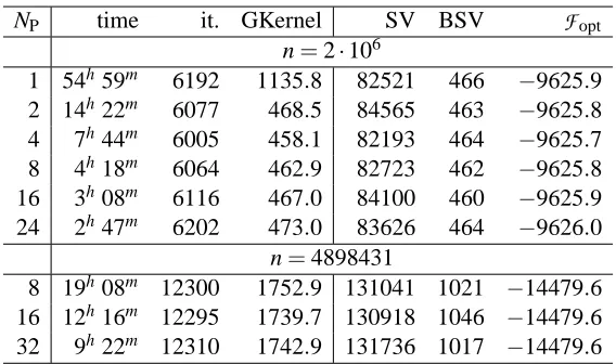
Table 4 shows the PGPDT performance in terms of training time and accuracy for different number of processors. Here, the time is measured in hours and minutes and the kernel evaluations are expressed in billions. For the test problem sized n=2·106, the serial results concern only the GPDT because LIBSVM exceeded the time limit of 60 hours and SVMlight stopped without a valid solution after relaxing the KKT conditions. Due to the very large size of the problem, the amount of 600MB for the caching area seems not sufficient to prevent a huge number of kernel evaluations in the serial run. Again, this drawback is reduced in the multiprocessor runs, due to increased memory for caching. Thus, analogously to some previous experiments (see Figures 4a, 5), superlinear speedup is exhibited, in this case up to about 20 processors. The largest test problem, with size about 5 millions and more than 105support vectors, can be faced in a reasonable time only with the parallel version. In this case the overall remark is that, on the considered architecture, few processors allow to train the Gaussian SVM in less than one day while few tens of processors can be exploited to reduce the training time to about 10 hours.
Finally, by observing in Table 4 the column of the objective function values, we may confirm that also in these experiments the training time saving ensured by PGPDT is obtained without damaging the solution accuracy.
These results show that PGPDT is able to exploit the resources of today multiprocessor systems to overcome the limits of the serial SVM implementations in solving O(106) problems (see also the training time in Figure 6a). As already mentioned, there is no other available parallel software to perform a fair comparison on the same architecture and the same data; however, an indirect comparison with the results reported by Graf et al. (2005) for the cascade algorithm suggests that PGPDT could be really competitive. Furthermore, since the cascade algorithm and PGPDT exploit very different parallelization ideas (recall that the former is based on the distribution of smaller independent SVMs), promising improvements could be achieved by an appropriate combination of the two approaches.
4. Conclusions and Future Work
NP time it. GKernel SV BSV
F
opt n=2·1061 54h59m 6192 1135.8 82521 466 −9625.9 2 14h22m 6077 468.5 84565 463 −9625.8 4 7h44m 6005 458.1 82193 464 −9625.7 8 4h18m 6064 462.9 82723 462 −9625.8 16 3h08m 6116 467.0 84100 460 −9625.9 24 2h47m 6202 473.0 83626 464 −9626.0
n=4898431
8 19h08m 12300 1752.9 131041 1021 −14479.6 16 12h16m 12295 1739.7 130918 1046 −14479.6 32 9h22m 12310 1742.9 131736 1017 −14479.6
Table 4: PGPDT scaling on very large test problems from the KDDCUP-99 data set.
serial SVM implementation currently available. The main improvements will concern: (i) the opti-mization/distribution of the tasks which are not currently parallelized, to improve the scalability; (ii) the introduction of a shrinking strategy, for further reducing the number of kernel evaluations; (iii) the inner solver robustness, to better face the subproblems arising from badly scaled training data. Furthermore, work is in progress to include in a new PGPDT release a suitable data distribution and the extension to regression problems.
Acknowledgments
The authors are grateful to the staff of the CINECA Supercomputing Center (Bologna, Italy) for supporting us with their valuable expertise. The authors also thank the anonymous referees for their helpful comments.
References
Jonathan Barzilai and Jonathan M. Borwein. Two-point step size gradient methods. IMA Journal of Numerical Analysis, 8(1):141–148, 1988.
Dimitri P. Bertsekas. Nonlinear Programming. Athena Scientific, Belmont, MA, second edition, 1999.
Ernesto G. Birgin, Jos´e Mario Mart´ınez, and Marcos Raydan. Nonmonotone spectral projected gradient methods on convex sets. SIAM Journal on Optimization, 10(4):1196–1211, 2000.
Bernhard E. Boser, Isabelle Guyon, and Vladimir N. Vapnik. A training algorithm for optimal margin classifiers. In David Haussler, editor, Proceedings of the 5th Annual ACM Workshop on Computational Learning Theory, pages 144–152. ACM Press, Pittsburgh, PA, 1992.
Chih-Chung Chang and Chih-Jen Lin. LIBSVM: a library for support vector machines, 2001. URL
Pai-Hsuen Chen, Rong-En Fan, and Chih-Jen Lin. A study on SMO-type decomposition methods for support vector machines. Technical report, Department of Computer Science and Information Engineering, National Taiwan University, Taipei, Taiwan, 2005. To appear on IEEE Transaction on Neural Networks, 2006.
Ronan Collobert and Samy Bengio. SVMTorch: Support vector machines for large-scale regression problems. Journal of Machine Learning Research, 1:143–160, 2001.
Ronan Collobert, Samy Bengio, and Yoshua Bengio. A parallel mixture of SVMs for very large scale problems. Neural Computation, 14(5):1105–1114, 2002.
Nello Cristianini and John Shawe-Taylor. An Introduction to Support Vector Machines and other Kernel-Based Learning Methods. Cambridge University Press, 2000.
Yu-Hong Dai and Roger Fletcher. New algorithms for singly linearly constrained quadratic pro-grams subject to lower and upper bounds. Mathematical Programming, 106(3):403–421, 2006.
Yu-Hong Dai and Roger Fletcher. Projected Barzilai-Borwein methods for large-scale box-constrained quadratic programming. Numerische Mathematik, 100(1):21–47, 2005.
Jian-Xiong Dong, Adam Krzyzak, and Ching Y. Suen. A fast parallel optimization for training support vector machine. In P. Perner and A. Rosenfeld, editors, Proceedings of 3rd International Conference on Machine Learning and Data Mining, volume 17, pages 96–105. Springer Lecture Notes in Artificial Intelligence, Leipzig, Germany, 2003.
Rong-En Fan, Pai-Hsuen Chen, and Chih-Jen Lin. Working set selection using second order in-formation for training Support Vector Machines. Journal of Machine Learning Research, 6: 1889–1918, 2005.
Hans Peter Graf, Eric Cosatto, L´eon Bottou, Igor Dourdanovic, and Vladimir N. Vapnik. Parallel support vector machines: the Cascade SVM. In Lawrence Saul, Yair Weiss, and L´eon Bottou, editors, Advances in Neural Information Processing Systems, volume 17. MIT Press, 2005.
Chih-Wei Hsu and Chih-Jen Lin. A simple decomposition method for support vector machines. Machine Learning, 46:291–314, 2002.
Don Hush and Clint Scovel. Polynomial-time decomposition algorithms for support vector ma-chines. Machine Learning, 51:51–71, 2003.
Throstem Joachims. Making large-scale SVM learning practical. In Bernard Sch¨olkopf, C.J.C. Burges, and Alex Smola, editors, Advances in Kernel Methods – Support Vector Learning. MIT Press, Cambridge, MA, 1998.
S. Sathiya Keerthi and Elmer G. Gilbert. Convergence of a generalized SMO algorithm for SVM classifier design. Machine Learning, 46:351–360, 2002.
Chih-Jen Lin. Linear convergence of a decomposition method for support vector machines. Tech-nical report, Department of Computer Science and Information Engineering, National Taiwan University, Taipei, Taiwan, 2001b.
Chih-Jen Lin. Asymptotic convergence of an SMO algorithm without any assumptions. IEEE Transactions on Neural Networks, 13:248–250, 2002.
Message Passing Interface Forum. MPI: A message-passing interface standard (version 1.2). Inter-national Journal of Supercomputing Applications, 8(3/4), 1995. URLhttp://www.mpi-forum. org. Also available as Technical Report CS-94-230, Computer Science Dept., University of Tennesse, Knoxville, TN.
Bruce A. Murtagh and Michael A. Saunders. MINOS 5.5 user’s guide. Technical report, Department of Operation Research, Stanford University, Stanford CA, 1998.
Edgar Osuna, Robert Freund, and Girosi Federico. Training support vector machines: an applica-tion to face detecapplica-tion. In Proceedings of the IEEE Conference on Computer Vision and Pattern Recognition (CVPR97), pages 130–136. IEEE Computer Society, New York, 1997.
Laura Palagi and Marco Sciandrone. On the convergence of a modified version of SVMlight algo-rithm. Optimization Methods and Software, 20:317–334, 2005.
Panos M. Pardalos and Naina Kovoor. An algorithm for a singly constrained class of quadratic programs subject to upper and lower bounds. Mathematical Programming, 46:321–328, 1990.
John C. Platt. Fast training of support vector machines using sequential minimal optimization. In Bernard Sch¨olkopf, C.J.C. Burges, and Alex Smola, editors, Advances in Kernel Methods – Support Vector Learning. MIT Press, Cambridge, MA, 1998.
Valeria Ruggiero and Luca Zanni. A modified projection algorithm for large strictly convex quadratic programs. Journal of Optimization Theory and Applications, 104(2):281–299, 2000a.
Valeria Ruggiero and Luca Zanni. Variable projection methods for large convex quadratic programs. In Donato Trigiante, editor, Recent Trends in Numerical Analysis, volume 3 of Advances in the Theory of Computational Mathematics, pages 299–313. Nova Science Publisher, 2000b.
Thomas Serafini and Luca Zanni. On the working set selection in gradient projection-based de-composition techniques for support vector machines. Optimization Methods and Software, 20: 583–596, 2005.
Thomas Serafini, Gaetano Zanghirati, and Luca Zanni. Gradient projection methods for quadratic programs and applications in training support vector machines. Optimization Methods and Soft-ware, 20:353–378, 2005.
Alex J. Smola. pr LOQO optimizer, 1997. URL http://www.kernel-machines.org/code/ prloqo.tar.gz.
Vladimir N. Vapnik. Statistical Learning Theory. John Wiley and Sons, New York, 1998.
Gaetano Zanghirati and Luca Zanni. A parallel solver for large quadratic programs in training support vector machines. Parallel Computing, 29:535–551, 2003.