Neural Autoregressive Distribution Estimation
Benigno Uria [email protected]
Google DeepMind London, UK
Marc-Alexandre Cˆot´e [email protected]
Department of Computer Science Universit´e de Sherbrooke
Sherbrooke, J1K 2R1, QC, Canada
Karol Gregor [email protected]
Google DeepMind London, UK
Iain Murray [email protected]
School of Informatics University of Edinburgh
Edinburgh EH8 9AB, UK
Hugo Larochelle [email protected]
141 Portland St, Floor 6 Cambridge MA 02139, USA
Editor:Ruslan Salakhutdinov
Abstract
We present Neural Autoregressive Distribution Estimation (NADE) models, which are neural network architectures applied to the problem of unsupervised distribution and density estimation. They leverage the probability product rule and a weight sharing scheme inspired from restricted Boltzmann machines, to yield an estimator that is both tractable and has good generalization performance. We discuss how they achieve competitive performance in modeling both binary and real-valued observations. We also present how deep NADE models can be trained to be agnostic to the ordering of input dimensions used by the autoregressive product rule decomposition. Finally, we also show how to exploit the topological structure of pixels in images using a deep convolutional architecture for NADE.
Keywords: deep learning, neural networks, density modeling, unsupervised learning
1. Introduction
Distribution estimation is one of the most general problems addressed by machine learning. From a good and flexible distribution estimator, in principle it is possible to solve a variety of types of inference problem, such as classification, regression, missing value imputation, and many other predictive tasks.
a latent statehfrom some prior p(h), followed by sampling the observed data xfrom some conditional p(x|h). Unfortunately, this approach quickly becomes intractable and requires approximations when the latent state h increases in complexity. Specifically, computing the marginal probability of the data,p(x) =P
hp(x|h)p(h), is only tractable under fairly
constraining assumptions on p(x|h) and p(h).
Another popular approach, based on undirected graphical models, gives probabilities of the formp(x) = exp{φ(x)}/Z, where φis a tractable function andZ is a normalizing con-stant. A popular choice for such a model is the restricted Boltzmann machine (RBM), which substantially out-performs mixture models on a variety of binary data sets (Salakhutdinov and Murray, 2008). Unfortunately, we often cannot compute probabilities p(x) exactly in undirected models either, due to the normalizing constantZ.
In this paper, we advocate a third approach to distribution estimation, based on autore-gressive models and feed-forward neural networks. We refer to our particular approach as Neural Autoregressive Distribution Estimation (NADE). Its main distinguishing property is that computingp(x) under a NADE model is tractable and can be computed efficiently, given an arbitrary ordering of the dimensions ofx.
The NADE framework was first introduced for binary variables by Larochelle and Murray (2011), and concurrent work by Gregor and LeCun (2011). The framework was then generalized to real-valued observations (Uria et al., 2013), and to versions based on deep neural networks that can model the observations in any order (Uria et al., 2014). This paper pulls together an extended treatement of these papers, with more experimental results, including some by Uria (2015). We also report new work on modeling 2D images by incorporating convolutional neural networks into the NADE framework. For each type of data, we’re able to reach competitive results, compared to popular directed and undirected graphical model alternatives.
2. NADE
We consider the problem of modeling the distributionp(x) of input vector observationsx. For now, we will assume that the dimensions of xare binary, that is xd∈ {0,1} ∀d. The
model generalizes to other data types, which is explored later (Section 3) and in other work (Section 8).
NADE begins with the observation that any D-dimensional distribution p(x) can be factored into a product of one-dimensional distributions, in any order o(a permutation of the integers 1, . . . , D):
p(x) =
D
Y
d=1
p(xod|xo<d). (1)
Here o<d contains the firstd−1 dimensions in ordering o and xo<d is the corresponding
subvector for these dimensions. Thus, one can define an ‘autoregressive’ generative model of the data simply by specifying a parameterization of allDconditionalsp(xod|xo<d).
conditional. Moreover, they allowed connections between the output of each network and the hidden layer of networks for the conditionals appearing earlier in the autoregressive ordering. Using neural networks led to some improvements in modeling performance, though at the cost of a really large model for very high-dimensional data.
In NADE, we also model each conditional using a feed-forward neural network. Specifi-cally, each conditionalp(xod|x<d) is parameterized as follows:
p(xod= 1|xo<d) = sigm (Vod,·hd+bod) (2) hd= sigm W·,o<dxo<d+c
, (3)
where sigm (a) = 1/(1 +e−a) is the logistic sigmoid, and withH as the number of hidden units, V ∈RD×H,b∈RD,W ∈RH×D,c∈RH are the parameters of the NADE model.
The hidden layer matrix W and biasc are shared by each hidden layerhd (which are all
of the same size). This parameter sharing scheme (illustrated in Figure 1) means that NADE has O(HD) parameters, rather thanO(HD2) required if the neural networks were separate. Limiting the number of parameters can reduce the risk of over-fitting. Another advantage is that allDhidden layers hdcan be computed in O(HD) time instead of O(HD2). Denoting
the pre-activation of thedthhidden layer asad=W·,o<dxo<d+c, this complexity is achieved
by using the recurrence
h1 = sigm (a1), wherea1 =c (4)
hd= sigm (ad), wheread=W·,o<dxo<d +c=W·,od−1xod−1 +ad−1 (5) ford∈ {2, . . . , D},
where Equation 5 given vector ad−1 can be computed in O(H). Moreover, the computation
of Equation 2 givenh is alsoO(H). Thus, computingp(x) from Dconditional distributions (Equation 1) costs O(HD) for NADE. This complexity is comparable to that of regular
feed-forward neural network models.
NADE can be trained by maximum likelihood, or equivalently by minimizing the average negative log-likelihood,
1
N N
X
n=1
−logp(x(n)) = 1
N N
X
n=1
D
X
d=1
−logp(x(on)
d |x (n)
o<d), (6)
usually by stochastic (minibatch) gradient descent. As probabilities p(x) cost O(HD), gradients of the negative log-probability of training examples can also be computed in
O(HD). Algorithm 1 describes the computation of bothp(x) and the gradients of−logp(x) with respect to NADE’s parameters.
2.1 Relationship with the RBM
The proposed weight-tying for NADE isn’t simply motivated by computational reasons. It also reflects the computations of approximation inference in the RBM.
Denoting the energy function and distribution under an RBM as
E(x,h) =−h>W x−b>x−c>h (7)
500 units
784 units
...
784 units ...
... ...
...
...
...
...
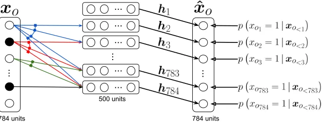
Figure 1: Illustration of a NADE model. In this example, in the input layer, units with value 0 are shown in black while units with value 1 are shown in white. The dashed border represents a layer pre-activation.The outputs ˆxO give predictive
probabilities for each dimension of a vector xO, given elements earlier in some
ordering. There is no path of connections between an output and the value being predicted, or elements of xO later in the ordering. Arrows connected together
correspond to connections with shared (tied) parameters.
computing all conditionals
p(xod|xo<d) =
X
xo>d∈{0,1}D−d X
h∈{0,1}H
exp{−E(x,h)}/Z(xo<d) (9)
Z(xo<d) =
X
xo≥d∈{0,1}D−d+1 X
h∈{0,1}H
exp{−E(x,h)} (10)
is intractable. However, these could be approximated using mean-field variational inference. Specifically, consider the conditional overxod,xo>d and hinstead:
p(xod,xo>d,h|xo<d) = exp{−E(x,h)}/Z(xo<d). (11)
A mean-field approach could first approximate this conditional with a factorized distribution
q(xod,xo>d,h|xo<d) =µi(d)
xod(1−µ
d(d))1−xod
Y
j>d
µj(d)xoj(1−µj(d))1−xoj
Y
k
τk(d)hk(1−τk(d))1−hk, (12)
where µj(d) is the marginal probability ofxoj being equal to 1, given xo<d. Similarly, τk(d)
is the marginal for hidden variablehk. The dependence on dcomes from conditioning on
xo<d, that is on the firstd−1 dimensions of xin ordering o.
For some d, a mean-field approximation is obtained by finding the parametersµj(d) for
j ∈ {d, . . . , D} and τk(d) for k∈ {1, . . . , H} which minimize the KL divergence between
Algorithm 1 Computation of p(x) and learning gradients for NADE.
Input: training observation vector xand orderingo of the input dimensions. Output: p(x) and gradients of −logp(x) on parameters.
# Computing p(x)
a1←c
p(x)←1
for dfrom 1 toDdo hd←sigm (ad)
p(xod= 1|xo<d)←sigm (Vod,·hd+bod)
p(x)←p(x) p(xod= 1|xo<d)
xod + (1−p(x
od= 1|xo<d)) 1−xod ad+1←ad+W·,odxod
end for
# Computing gradients of −logp(x)
δaD ←0
δc←0
for dfromD to 1do
δbod ← p(xod= 1|xo<d)−xod
δVod,·← p(xod= 1|xo<d)−xod
h>d
δhd← p(xod= 1|xo<d)−xod
Vo>d,·
δc←δc+δhdhd(1−hd)
δW·,od ←δadxod
δad−1←δad+δhdhd(1−hd)
end for
return p(x), δb, δV, δc, δW
passing updates that each set the derivatives of the KL divergence to 0 for some of the parameters ofq(xod,xo>d,h|xo<d) given others.
For some d, let us fix µj(d) =xod for j < d, leaving only µj(d) for j > d to be found.
The KL-divergence develops as follows:
KL(q(xod,xo>d,h|xo<d)||p(xod,xo>d,h|xo<d))
= − X
xod,xo>d,h
q(xod,xo>d,h|xo<d) logp(xod,xo>d,h|xo<d)
+ X
xod,xo>d,h
q(xod,xo>d,h|xo<d) logq(xod,xo>d,h|xo<d)
= logZ(xo<d)− X
j
X
k
τk(d)Wk,ojµj(d)− X
j
bojµj(d)− X
k
ckτk(d)
+X
j≥d
(µj(d) logµj(d) + (1−µj(d)) log(1−µj(d)))
+X
k
Then, we can take the derivative with respect to τk(d) and set it to 0, to obtain:
0 = ∂KL(q(xod,xo>d,h|xo<d)||p(xod,xo>d,h|xo<d))
∂τk(d)
0 = −ck−
X
j
Wk,ojµj(d) + log
τk(d)
1−τk(d)
τk(d)
1−τk(d)
= exp
ck+
X
j
Wk,ojµj(d)
(13)
τk(d) =
expnck+PjWk,ojµj(d) o
1 + expnck+PjWk,ojµj(d) o
τk(d) = sigm
ck+
X
j≥d
Wk,ojµj(d) + X
j<d
Wk,ojxoj
. (14)
where in the last step we have used the fact that µj(d) =xoj for j < d. Equation 14 would
correspond to the message passing updates of the hidden unit marginals τk(d) given the
marginals of input µj(d).
Similarly, we can set the derivative with respect toµj(d) for j≥dto 0 and obtain:
0 = ∂KL(q(xod,xo>d,h|xo<d)||p(xod,xo>d,h|xo<d))
∂µj(d)
0 = −bod− X
k
τk(d)Wk,oj+ log
µj(d)
1−µj(d)
µj(d)
1−µj(d)
= exp
(
boj+ X
k
τk(d)Wk,oj )
µj(d) =
expboj+ P
kτk(d)Wk,oj
1 + expboj + P
kτk(d)Wk,oj
µj(d) = sigm boj+
X
k
τk(d)Wk,oj !
. (15)
Equation 15 would correspond to the message passing updates of the input marginalsµj(d)
given the hidden layer marginals τk(d). The complete mean-field algorithm would thus
alternate between applying the updates of Equations 14 and 15, right to left.
We now notice that Equation 14 corresponds to NADE’s hidden layer computation (Equation 3) whereµj(d) = 0 ∀j≥d. Also, Equation 15 corresponds to NADE’s output
layer computation (Equation 2) where j=d,τk(d) =hd,k and W> =V. Thus, in short,
NADE’s forward pass is equivalent to applying a single pass of mean-field inference to approximate all the conditionals p(xod|xo<d) of an RBM, where initially µj(d) = 0 and
3. NADE for Non-Binary Observations
So far we have only considered the case of binary observationsxi. However, the framework
of NADE naturally extends to distributions over other types of observations.
In the next section, we discuss the case of real-valued observations, which is one of the most general cases of non-binary observations and provides an illustrative example of the technical considerations one faces when extending NADE to new observations.
3.1 RNADE: Real-Valued NADE
A NADE model for real-valued data could be obtained by applying the derivations shown in Section 2.1 to the Gaussian-RBM (Welling et al., 2005). The resulting neural network would output the mean of a Gaussian with fixed variance for each of the conditionals in Equation 1. Such a model is not competitive with mixture models, for example on perceptual data sets (Uria, 2015). However, we can explore alternative models by making the neural network for each conditional distribution output the parameters of a distribution that’s not a fixed-variance Gaussian.
In particular, a mixture of one-dimensional Gaussians for each autoregressive conditional provides a flexible model. Given enough components, a mixture of Gaussians can model any continuous distribution to arbitrary precision. The resulting model can be interpreted as a sequence of mixture density networks (Bishop, 1994) with shared parameters. We call this model RNADE-MoG. In RNADE-MoG, each of the conditionals is modeled by a mixture of Gaussians:
p(xod|xo<d) =
C
X
c=1
πod,c N(xod;µod,c, σ 2
od,c), (16)
where the parameters are set by the outputs of a neural network:
πod,c=
expnzo(πd,c) o
PC
c=1exp n
z(oπd,c)
o (17)
µod,c=z (µ)
od,c (18)
σod,c= exp n
zo(σd),co (19)
zo(πd,c) =b(oπd),c+
H
X
k=1
Vo(π)
d,k,chd,k (20)
zo(µd,c) =b(oµd),c+
H
X
k=1
Vo(µ)
d,k,chd,k (21)
zo(σd,c) =b(oσd),c+
H
X
k=1
Vo(σ)
d,k,chd,k (22)
Different one dimensional conditional forms may be preferred, for example due to limited data set size or domain knowledge about the form of the conditional distributions. Other choices, like single variable-variance Gaussians, sinh-arcsinh distributions, and mixtures of Laplace distributions, have been examined by Uria (2015).
Training an RNADE can still be done by stochastic gradient descent on the parameters of the model with respect to the negative log-density of the training set. It was found empirically (Uria et al., 2013) that stochastic gradient descent leads to better parameter configurations when the gradient of the mean ∂µ∂J
od,c
was multiplied by the standard
deviation (σod,c).
4. Orderless and Deep NADE
The fixed ordering of the variables in a NADE model makes the exact calculation of arbitrary conditional probabilities computationally intractable. Only a small subset of conditional distributions, those where the conditioned variables are at the beginning of the ordering and marginalized variables at the end, are computationally tractable.
Another limitation of NADE is that a naive extension to a deep version, with multiple layers of hidden units, is computationally expensive. Deep neural networks (Bengio, 2009; LeCun et al., 2015) are at the core of state-of-the-art models for supervised tasks like image recognition (Krizhevsky et al., 2012) and speech recognition (Dahl et al., 2013). The same inductive bias should also provide better unsupervised models. However, extending the NADE framework to network architectures with several hidden layers, by introducing extra non-linear calculations between Equations 3 and 2, increases its complexity to cubic in the number of units per layer. Specifically, the cost becomesO(DH2L), where Lstands for the number of hidden layers and can be assumed to be a small constant,D is the number of variables modeled, andH is the number of hidden units, which we assumed to be of the same order as D. This increase in complexity is caused by no longer being able to share hidden layer computations across the conditionals in Equation 1, after the non-linearity in the first layer.
We first describe the model for an L-layer neural network modeling binary variables. A conditional distribution is obtained directly from a hidden unit in the final layer:
p(xod= 1|xo<d,θ, o<d, od) =h (L)
od . (23)
This hidden unit is computed from previous layers, all of which can only depend on thexo<d
variables that are currently being conditioned on. We remove the other variables from the computation using a binary mask,
mo<d = [11∈o<d,12∈o<d, . . . ,1D∈o<d], (24)
which is element-wise multiplied with the inputs before computing the remaining layers as in a standard neural network:
h(0) =xmo<d (25) a(`)=W(`)h(`−1)+b(`) (26)
h(`)=σ
a(`)
(27)
h(L)=sigma(L). (28) The network is specified by a free choice of the activation function σ(·), and learnable parametersW(`)∈RH(`)×H(`
−1)
andb(`)∈RH(`), whereH(l) is the number of units in the
`-th layer. As layer zero is the masked input,H(0)=D. The final L-th layer needs to be able to provide predictions for any element (Equation 23) and so also hasD units.
To train a DeepNADE, the ordering of the variables is treated as a stochastic variable with a uniform distribution. Moreover, since we wish DeepNADE to provide good predictions for any ordering, we optimize the expected likelihood over the ordering of variables:
J(θ) = E
o∈D!−logp(X|θ, o)∝o∈ED!xE∈X−logp(x|θ, o), (29) where we’ve made the dependence on the orderingoand the network’s parametersθ explicit,
D! stands for the set of all orderings (the permutations ofD elements) andxis a uniformly sampled data point from the training setX. Using NADE’s expression for the density of a data point in Equation 1 we have
J(θ) = E
o∈D!xE∈X D
X
d=1
−logp(xod|xo<d,θ, o), (30)
where dindexes the elements in the ordering,o, of the variables. By moving the expectation over orderings inside the sum over the elements of the ordering, the ordering can be split in three parts: o<d (the indices of the d−1 first dimensions in the ordering),od (the index of
the d-th variable) and o>d (the indices of the remaining dimensions). Therefore, the loss
function can be rewritten as:
J(θ) = E
x∈X D
X
d=1 E
o<dEodoE>d
The value of each of these terms does not depend on o>d. Therefore, it can be simplified as:
J(θ) = E
x∈X D
X
d=1 E
o<doEd−
logp(xod|xo<d,θ, o<d, od). (32)
In practice, this loss function will have a very high number of terms and will have to be approximated by sampling x,dando<d. The innermost expectation over values of od
can be calculated cheaply, because all of the neural network computations depend only on the masked input xo<d, and can be reused for each possible od. Assuming all orderings are
equally probable, we will estimate J(θ) by:
b
J(θ) = D
D−d+ 1
X
od
−logp(xod|xo<d,θ, o<d, od), (33)
which is an unbiased estimator of Equation 29. Therefore, training can be done by descent on the gradient of Jb(θ).
For binary observations, we use the cross-entropy scaled by a factor of D−Dd+1 as the training loss which corresponds to minimizingJb:
J(x) = D
D−d+ 1 m
> o≥d
xlogh(L)+ (1−x)log1−h(L). (34) Differentiating this cost involves backpropagating the gradients of the cross-entropy only from the outputs ino≥d and rescaling them by D−Dd+1.
The resulting training procedure resembles that of a denoising autoencoder (Vincent et al., 2008). Like the autoencoder,D outputs are used to predictD inputs corrupted by a random masking process (mo<d in Equation 25). A single forward pass can compute h
(L)
o≥d,
which provides a prediction p(xod= 1|xo<d,θ, o<d, od) for every masked variable, which
could be used next in an ordering starting witho<d. Unlike the autoencoder, the outputs
for variables corresponding to those provided in the input (not masked out) are ignored. In this order-agnostic framework, missing variables and zero-valued observations are indistinguishable by the network. This shortcoming can be alleviated by concatenating the inputs to the network (masked variables xmo<d) with the mask mo<d. Therefore we
advise substituting the input described in Equation 25 with
h(0) = concat(xmo<d,mo<d). (35)
We found this modification to be important in order to obtain competitive statistical performance (see Table 3). The resulting neural network is illustrated in Figure 2.
4.1 Ensembles of NADE Models
...
500 units
...
500 units
...
784 units
...
784 units
...
784 units
...
784 units
1568 units
...
...
...
784 units
Figure 2: Illustration of a DeepNADE model with two hidden layers. The dashed border represents a layer pre-activation. Units with value 0 are shown in black while units with value 1 are shown in white. A maskmo<d specifies a subset of variables
to condition on. A conditional or predictive probability of the remaining variables is given in the final layer. The output units with a corresponding input mask of value 1 (shown with dotted contour) are not involved in DeepNADE’s training loss (Equation 34).
However, it is possible to use this variability across the different orderings to our advantage by combining several models. A usual approach to improve on a particular estimator is to construct an ensemble of multiple, strong but different estimators, e.g. using bagging (Ormoneit and Tresp, 1995) or stacking (Smyth and Wolpert, 1999). The DeepNADE training procedure suggests a way of generating ensembles of NADE models: take a set of uniformly distributed orderings {o(k)}Kk=1 over the input variables and use the average probability K1 PK
k=1p(x|θ, o(k)) as an estimator.
The use of an ensemble increases the test-time cost of density estimation linearly with the number of orderings used. The complexity of sampling does not change however: after one of theK orderings is chosen at random, the single corresponding NADE is sampled. Importantly, the cost of training also remains the same, unlike other ensemble methods such as bagging. Furthermore, the number of components can be chosen after training and even adapted to a computational budget on the fly.
5. ConvNADE: Convolutional NADE
Recently, convolutional neural networks (CNN) have achieved state-of-the-art perfor-mance on many supervised tasks related to images Krizhevsky et al. (2012). Briefly, CNNs are composed of convolutional layers, each one having multiple learnable filters. The outputs of a convolutional layer are feature maps and are obtained by the convolution on the input image (or previous feature maps) of a linear filter, followed by the addition of a bias and the application of a non-linear activation function. Thanks to the convolution, spatial structure in the input is preserved and can be exploited. Moreover, as per the definition of a convolution the same filter is reused across all sub-regions of the entire image (or previous feature maps), yielding a parameter sharing that is natural and sensible for images.
The success of CNNs raises the question: can we exploit the spatial topology of the inputs while keeping NADE’s autoregressive property? It turns out we can, simply by replacing the fully connected hidden layers of a DeepNADE model with convolutional layers. We thus refer to this variant as Convolutional NADE (ConvNADE).
First we establish some notation that we will use throughout this section. Without loss of generality, let the inputX ∈ {0,1}NX×NX be a square binary image of sizeN
X and every
convolution filter W(ij`) ∈ RN
(`)
W×N
(`)
W connecting two feature maps H(`−1)
i and H
(`)
j also
be square with their sizeNW(`) varying for each layer `. We also define the following mask
Mo<d ∈ {0,1}
NX×NX, which is 1 for the locations of the firstd−1 pixels in the ordering o.
Formally, Equation 26 is modified to use convolutions instead of dot products. Specifically for anL-layer convolutional neural network that preserves the input shape (explained below) we have
p(xod= 1|xo<d,θ, o<d, od) =vec
H(1L)
od
, (36)
with
H(0)1 =XMo<d (37) A(j`) =b(j`)+
H(`−1)
X
i=1
H(i`−1)~W(ij`) (38)
H(j`) =σA(j`) (39)
H(jL) =sigm
A(jL)
, (40)
where H(`) is the number of feature maps output by the `-th layer and b(l) ∈ RH(l), W(`)∈RH
(`−1)×H(`)×N(`)
W×N
(`)
W , withdenoting the element-wise multiplication, σ(·) being
any activation function andvec(X)→xis the concatenation of every row inX. Note that
H(0) corresponds to the number of channels the input images have.
For notational convenience, we use ~ to denote both “valid” convolutions and “full” convolutions, instead of introducing bulky notations to differentiate these cases. The “valid” convolutions only apply a filter to complete patches of the image, resulting in a smaller image (its shape is decreased toNX −NW(`)+ 1). Alternatively, “full” convolutions zero-pad the
contour of the image before applying the convolution, thus expanding the image (its shape is increased toNX +NW(`)−1). Which one is used should be self-explanatory depending on
Moreover, in order for ConvNADE to output conditional probabilities as shown in Equation 36, the output layer must have only one feature map H(1L), whose dimension matches the dimension of the input X. This can be achieved by carefully combining layers that use either “valid” or “full” convolutions.
To explore different model architectures respecting that constraint, we opted for the following strategy. Given a network, we ensured the first half of its layers was using “valid” convolutions while the other half would use “full” convolutions. In addition to that, we made sure the network was symmetric with respect to its filter shapes (i.e. the filter shape used in layer`matched the one used in layerL−`).
For completeness, we wish to mention that ConvNADE can also include pooling and upsampling layers, but we did not see much improvement when using them. In fact, recent research suggests that these types of layers are not essential to obtain state-of-the-art results (Springenberg et al., 2015).
The flexibility of DeepNADE allows us to easily combine both convolutional and fully connected layers. To create such hybrid models, we used the simple strategy of having two separate networks, with their last layer fused together at the end. The ‘convnet’ part is only composed of convolutional layers whereas the ‘fullnet’ part is only composed of fully connected layers. The forward pass of both networks follows respectively Equations 37–39 and Equations 25–27. Note that in the ‘fullnet’ network case,xcorresponds to the input image having been flattened.
In the end, the output layer g of the hybrid model corresponds to the aggregation of the last layer pre-activation of both ‘convnet’ and ‘fullnet’ networks. The conditionals are slightly modified as follows:
p(xod= 1|xo<d,θ, o<d, od) =god (41)
g =sigmvecA1(L)+a(L). (42) The same training procedure as for DeepNADE model can also be used for ConvNADE. For binary observations, the training loss is similar to Equation 34, with h(L) being substi-tuted for g as defined in Equation 42.
As for the DeepNADE model, we found that providing the mask Mo<d as an input
to the model improves performance (see Table 4). For the ‘convnet’ part, the mask was provided as an additional channel to the input layer. For the ‘fullnet’ part, the inputs were concatenated with the mask as shown in Equation 35.
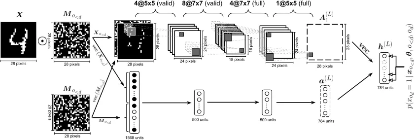
The final architecture is shown in Figure 3. In our experiments, we found that this type of hybrid model works better than only using convolutional layers (see Table 4). Certainly, more complex architectures could be employed but this is a topic left for future work.
6. Related Work
As we mentioned earlier, the development of NADE and its extensions was motivated by the question of whether a tractable distribution estimator could be designed to match a powerful but intractable model such as the restricted Boltzmann machine.
...
784 units 24 pixels
24 pixels
28 pixels
28 pixels
...
500 units
28 pixels
28 pixels ...
500 units
28 pixels
28 pixels
24 pixels
24 pixels
18 pixels
18 pixels
4@5x5 (valid) 8@7x7 (valid) 4@7x7 (full) 1@5x5 (full)
...
784 units 28 pixels
28 pixels
1568 units
...
...
28 pixels
28 pixels
Figure 3: Illustration of a ConvNADE that combines a convolutional neural network with three hidden layers and a fully connected feed-forward neural network with two hidden layers. The dashed border represents a layer pre-activation. Units with a dotted contour are not valid conditionals since they depend on themselves i.e. they were given in the input.
competitive, despite the simplicity of the distribution family for its conditionals. Bengio and Bengio (2000) later proposed using more powerful conditionals, modeled as single layer neural networks. Moreover, they proposed connecting the output of eachdth conditional to all of the hidden layers of thed−1 neural networks for the preceding conditionals. More recently, Germain et al. (2015) generalized this model by deriving a simple procedure for making it deep and orderless (akin to DeepNADE, in Section 4). We compare with all of these approaches in Section 7.1.
There exists, of course, more classical and non-autoregressive approaches to tractable distribution estimation, such as mixture models and Chow–Liu trees (Chow and Liu, 1968). We compare with these as well in Section 7.1.
This work also relates directly to the recently growing literature on generative neural networks. In addition to the autoregressive approach described in this paper, there exists three other types of such models: directed generative networks, undirected generative networks and hybrid networks.
posterior. The VAE optimizes a bound on the likelihood which is estimated using a single sample from the variational posterior, though recent work has shown that a better bound can be obtained using an importance sampling approach (Burda et al., 2016). Gregor et al. (2015) later exploited the VAE approach to develop DRAW, a directed generative model for images based on a read-write attentional mechanism. Goodfellow et al. (2014) proposed an adversarial approach to training directed generative networks, that relies on a discriminator network simultaneously trained to distinguish between data and model samples. Generative networks trained this way are referred to as Generative Adversarial Networks (GAN). While the VAE optimizes a bound of the likelihood (which is the KL divergence between the empirical and model distributions), it can be shown that the earliest versions of GANs optimize the Jensen–Shannon (JS) divergence between the empirical and model distributions. Li et al. (2015) instead propose a training objective derived from Maximum Mean Discrepancy (MMD; Gretton et al., 2007). Recently, the directed generative model approach has been very successfully applied to model images (Denton et al., 2015; Sohl-Dickstein et al., 2011).
The undirected paradigm has also been explored extensively for developing powerful gen-erative networks. These include the restricted Boltzmann machine (Smolensky, 1986; Freund and Haussler, 1992) and its multilayer extension, the deep Boltzmann machine (Salakhut-dinov and Hinton, 2009), which dominate the literature on undirected neural networks. Salakhutdinov and Murray (2008) provided one of the first quantitative evidence of the generative modeling power of RBMs, which motivated the original parameterization for NADE (Larochelle and Murray, 2011). Efforts to train better undirected models can vary in nature. One has been to develop alternative objectives to maximum likelihood. The proposal of Contrastive Divergence (CD; Hinton, 2002) was instrumental in the popularization of the RBM. Other proposals include pseudo-likelihood (Besag, 1975; Marlin et al., 2010), score matching (Hyv¨arinen, 2005; Hyv¨arinen, 2007a,b), noise contrastive estimation (Gutmann and Hyv¨arinen, 2010) and probability flow minimization (Sohl-Dickstein et al., 2011). An-other line of development has been to optimize likelihood using Robbins–Monro stochastic approximation (Younes, 1989), also known as Persistent CD (Tieleman, 2008), and develop good MCMC samplers for deep undirected models (Salakhutdinov, 2009, 2010; Desjardins et al., 2010; Cho et al., 2010). Work has also been directed towards proposing improved update rules or parameterization of the model’s energy function (Tieleman and Hinton, 2009; Cho et al., 2013; Montavon and M¨uller, 2012) as well as improved approximate inference of the hidden layers (Salakhutdinov and Larochelle, 2010). The work of Ngiam et al. (2011) also proposed an undirected model that distinguishes itself from deep Boltzmann machines by having deterministic hidden units, instead of stochastic.
Finally, hybrids of directed and undirected networks are also possible, though much less common. The most notable case is the Deep Belief Network (DBN; Hinton et al., 2006), which corresponds to a sigmoid belief network for which the prior over its top hidden layer is an RBM (whose hidden layer counts as an additional hidden layer). The DBN revived interest in RBMs, as they were required to successfully initialize the DBN.
Name # Inputs Train Valid. Test
Adult 123 5000 1414 26147
Connect4 126 16000 4000 47557
DNA 180 1400 600 1186
Mushrooms 112 2000 500 5624
NIPS-0-12 500 400 100 1240
OCR-letters 128 32152 10000 10000
RCV1 150 40000 10000 150000
Web 300 14000 3188 32561
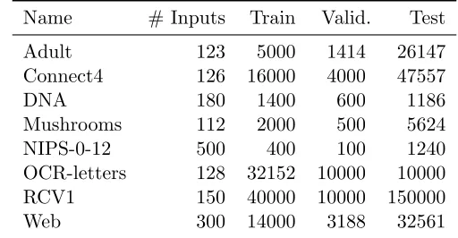
Table 1: Statistics on the binary vector data sets of Section 7.1.
exact samples from the model (unlike in undirected models) and get an unbiased gradient for maximum likelihood training (unlike in directed graphical models).
7. Results
In this section, we evaluate the performance of our different NADE models on a variety of data sets. The code to reproduce the experiments of the paper is available on GitHub1. Our implementation is done using Theano (Team et al., 2016).
7.1 Binary Vectors Data Sets
We start by evaluating the performance of NADE models on a set of benchmark data sets where the observations correspond to binary vectors. These data sets were mostly taken from the LIBSVM data sets web site2, except for OCR-letters3 and NIPS-0-124. Code to download these data sets is available here: http://info.usherbrooke.ca/hlarochelle/ code/nade.tar.gz. Table 1 summarizes the main statistics for these data sets.
For these experiments, we only consider tractable distribution estimators, where we can evaluatep(x) on test items exactly. We consider the following baselines:
• MoB: A mixture of multivariate Bernoullis, trained using the EM algorithm. The number of mixture components was chosen from{32,64,128,256,512,1024} based on validation set performance, and early stopping was used to determine the number of EM iterations.
• RBM: A restricted Boltzmann machine made tractable by using only 23 hidden units, trained by contrastive divergence with up to 25 steps of Gibbs sampling. The validation set performance was used to select the learning rate from {0.005,0.0005,0.00005}, and the number of iterations over the training set from {100,500,1000}.
1.http://github.com/MarcCote/NADE
2.http://www.csie.ntu.edu.tw/~cjlin/libsvmtools/datasets/ 3.http://ai.stanford.edu/~btaskar/ocr/
• FVSBN: Fully visible sigmoid belief network, that models each conditionalp(xod|xo<d)
with logistic regression. The ordering of inputs was selected randomly. Training was by stochastic gradient descent. The validation set was used for early stopping, as well as for choosing the base learning rateη∈ {0.05,0.005,0.0005}, and a decreasing schedule constantγ from {0,0.001,0.000001}for the learning rate schedule η/(1 +γt) for the
tth update.
• Chow–Liu: A Chow–Liu tree is a graph over the observed variables, where the distribution of each variable, except the root, depends on a single parent node. There is an O(D2) fitting algorithm to find the maximum likelihood tree and conditional distributions (Chow and Liu, 1968). We adapted an implementation provided by Harmeling and Williams (2011), who found Chow–Liu to be a strong baseline.
The maximum likelihood parameters are not defined when conditioning on events that haven’t occurred in the training set. Moreover, conditional probabilities of zero are possible, which could give infinitely bad test set performance. We re-estimated the conditional probabilities on the Chow–Liu tree using Lidstone or “add-α” smoothing:
p(xd= 1|xparent=z) =
count(xd= 1|xparent=z) +α
count(xparent=z) + 2α
, (43)
selecting α for each data set from{10−20,0.001,0.01,0.1} based on performance on the validation set.
• MADE (Germain et al., 2015): Generalization of the neural network approach of Bengio and Bengio (2000), to multiple layers. We consider a version using a single (fixed) input ordering and another trained on multiple orderings from which an ensemble was constructed (which was inspired from the order-agnostic approach of Section 4) that we refer to as MADE-E. See Germain et al. (2015) for more details.
We compare these baselines with the two following NADE variants:
• NADE (fixed order): Single layer NADE model, trained on a single (fixed) randomly generated order, as described in Section 2. The sigmoid activation function was used for the hidden layer, of size 500. Much like for FVSBN, training relied on stochastic gradient descent and the validation set was used for early stopping, as well as for choosing the learning rate from {0.05, 0.005, 0.0005}, and the decreasing schedule constantγ from{0,0.001,0.000001}.
Model Adult Connect4 DNA Mushrooms NIPS-0-12 OCR-letters RCV1 Web
MoB -20.44 -23.41 -98.19 -14.46 -290.02 -40.56 -47.59 -30.16 RBM -16.26 -22.66 -96.74 -15.15 -277.37 -43.05 -48.88 -29.38 FVSBN -13.17 -12.39 -83.64 -10.27 -276.88 -39.30 -49.84 -29.35 Chow–Liu -18.51 -20.57 -87.72 -20.99 -281.01 -48.87 -55.60 -33.92 MADE -13.12 -11.90 -83.63 -9.68 -280.25 -28.34 -47.10 -28.53 MADE-E -13.13 -11.90 -79.66 -9.69 -277.28 -30.04 -46.74 -28.25
NADE -13.19 -11.99 -84.81 -9.81 -273.08 -27.22 -46.66 -28.39 NADE-E -13.19 -12.58 -82.31 -9.69 -272.39 -27.32 -46.12 -27.87
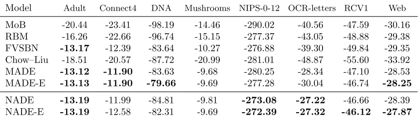
Table 2: Average log-likelihood performance of tractable distribution baselines and NADE models, on binary vector data sets. The best result is shown in bold, along with any other result with an overlapping confidence interval.
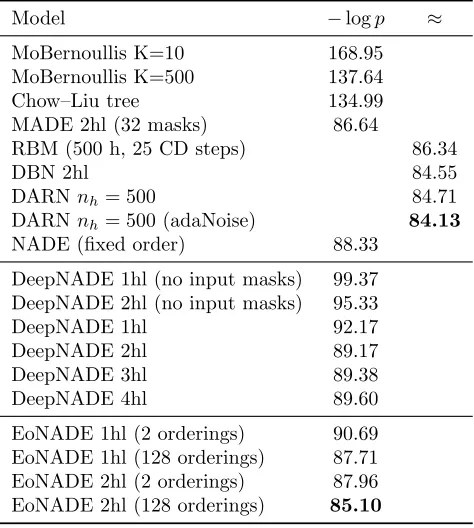
Table 2 presents the results. We observe that NADE restricted to a fixed ordering of the inputs achieves very competitive performance compared to the baselines. However, the order-agnostic version of NADE is overall the best method, being among the top performing model for 5 data sets out of 8.
The performance of fixed-order NADE is surprisingly robust to variations of the chosen input ordering. The standard deviation on the average log-likelihood when varying the ordering was small: on Mushrooms, DNA and NIPS-0-12, we observed standard deviations of 0.045, 0.05 and 0.15, respectively. However, models with different orders can do well on different test examples, which explains why ensembling can still help.
7.2 Binary Image Data Set
We now consider the case of an image data set, constructed by binarizing the MNIST digit data set. Each image has been stochastically binarized according to their pixel intensity as generated by Salakhutdinov and Murray (2008). This benchmark has been a popular choice for the evaluation of generative neural network models. Here, we investigate two questions:
1. How does NADE compare to intractable generative models?
2. Does the use of a convolutional architecture improve the performance of NADE?
For these experiments, in addition to the baselines already described in Section 7.1, we consider the following:
• DARN (Gregor et al., 2014): This deep generative autoencoder has two hidden layers, one deterministic and one with binary stochastic units. Both layers have 500 units (denoted as nh = 500). Adaptive weight noise (adaNoise) was either used or
Model −logp ≈
MoBernoullis K=10 168.95 MoBernoullis K=500 137.64
Chow–Liu tree 134.99
MADE 2hl (32 masks) 86.64
RBM (500 h, 25 CD steps) 86.34
DBN 2hl 84.55
DARN nh= 500 84.71
DARN nh= 500 (adaNoise) 84.13 NADE (fixed order) 88.33
DeepNADE 1hl (no input masks) 99.37 DeepNADE 2hl (no input masks) 95.33
DeepNADE 1hl 92.17
DeepNADE 2hl 89.17
DeepNADE 3hl 89.38
DeepNADE 4hl 89.60
EoNADE 1hl (2 orderings) 90.69 EoNADE 1hl (128 orderings) 87.71 EoNADE 2hl (2 orderings) 87.96 EoNADE 2hl (128 orderings) 85.10
Table 3: Negative log-likelihood test results of models ignorant of the 2D topology on the binarized MNIST data set.
• DRAW (Gregor et al., 2015): Similar to a variational autoencoder where both the encoder and the decoder are LSTMs, guided (or not) by an attention mechanism. In this model, both LSTMs (encoder and decoder) are composed of 256 recurrent hidden units and always perform 64 timesteps. When the attention mechanism is enabled, patches (2×2 pixels) are provided as inputs to the encoder instead of the whole image and the decoder also produces patches (5×5 pixels) instead of a whole image.
• Pixel RNN(Oord et al., 2016): NADE-like model for natural images that is based on convolutional and LSTM hidden units. This model has 7 hidden layers, each composed of 16 units. Oord et al. (2016) proposed a novel two-dimensional LSTM, named Diagonal BiLSTM, which is used in this model. Unlike our ConvNADE, the ordering is fixed before training and at test time, and corresponds to a scan of the image in a diagonal fashion starting from a corner at the top and reaching the opposite corner at the bottom.
We compare these baselines with some NADE variants. The performance of a basic (fixed-order, single hidden layer) NADE model is provided in Table 3 and samples are illustrated in Figure 4. More importantly, we will focus on whether the following variants achieve better test set performance:
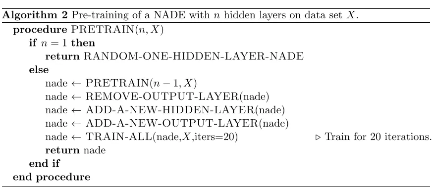
was either provided or not (no input masks) to the model. The rectified linear activation function was used for all hidden layers. Minibatch gradient descent was used for training, with minibatches of size 1000. Training consisted of 200 iterations of 1000 parameter updates. Each hidden layer was pre-trained according to Algorithm 2. We report an average of the average test log-likelihoods over ten different random orderings.
• EoNADE: This variant is similar to DeepNADE except for the log-likelihood on the test set, which is instead computed from an ensemble that averages predictive probabilities over 2 or 128 orderings. To clarify, the DeepNADE results report the typical performance of one ordering, by averaging results after taking the log, and so do not combine the predictions of the models like EoNADE does.
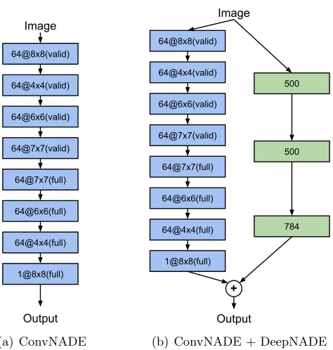
• ConvNADE: Multiple convolutional layers trained according to the order-agnostic procedure described in Section 4. The exact architecture is shown in Figure 5(a). Information about which inputs are masked was either provided or not (no input masks). The rectified linear activation function was used for all hidden layers. The Adam optimizer (Kingma and Ba, 2015) was used with a learning rate of 10−4. Early stopping was used with a look ahead of 10 epochs, using Equation 34 to get a stochastic estimate of the validation set average log-likelihood. An ensemble using 128 orderings was used to compute the log-likelihood on the test set.
• ConvNADE + DeepNADE: This variant is similar to ConvNADE except for the aggregation of a separate DeepNADE model at the end of the network. The exact architecture is shown in Figure 5(b). The training procedure is the same as with ConvNADE.
Algorithm 2 Pre-training of a NADE withn hidden layers on data setX. procedure PRETRAIN(n, X)
if n= 1 then
return RANDOM-ONE-HIDDEN-LAYER-NADE
else
nade ←PRETRAIN(n−1, X)
nade ←REMOVE-OUTPUT-LAYER(nade)
nade ←ADD-A-NEW-HIDDEN-LAYER(nade)
nade ←ADD-A-NEW-OUTPUT-LAYER(nade)
nade ←TRAIN-ALL(nade,X,iters=20) .Train for 20 iterations.
return nade end if
end procedure
Figure 2: (Left): samples from NADE trained on a binary version of mnist. (Middle): probabilities from
which each pixel was sampled. (Right): visualization of some of the rows of W. This figure is better seen on a
computer screen.
set it to 0, to obtain:
0 = ∂KL(q(vi,v>i,h|v<i)||p(vi,v>i,h|v<i))
∂τk(i)
0 = −ck−Wk,·µ(i) + log
τk(i)
1−τk(i)
τk(i)
1−τk(i)
= exp(ck+Wk,·µ(i))
τk(i) =
exp(ck+Wk,·µ(i))
1 + exp(ck+Wk,·µ(i))
τk(i) = sigm
ck+
X
j≥i
Wkjµj(i) +
X
j<i
Wkjvj
where in the last step we have replaced the
ma-trix/vector multiplicationWk,·µ(i) by its explicit
sum-mation form and have used the fact thatµj(i) = vj for
j < i.
Similarly, we set the derivative with respect to µj(i)
for j ≥i to 0 and obtain:
0 = ∂KL(q(vi,v>i,h|v<i)||p(vi,v>i,h|v<i))
∂µj(i)
0 = −bj−τ(i)>W·,j+ log
µj(i)
1−µj(i)
µj(i)
1−µj(i)
= exp(bj+τ(i)>W·,j)
µj(i) =
exp(bj +τ(i)>W·,j)
1 + exp(bj+τ(i)>W·,j)
µj(i) = sigm bj+
X
k
Wkjτk(i)
!
We then recover the mean-field updates of
Equa-tions 7 and 8.
References
Bengio, Y., & Bengio, S. (2000). Modeling high-dimensional discrete data with multi-layer neural
networks. Advances in Neural Information
Process-ing Systems 12 (NIPS’99)(pp. 400–406). MIT Press.
Bengio, Y., Lamblin, P., Popovici, D., & Larochelle, H. (2007). Greedy layer-wise training of deep networks.
Advances in Neural Information Processing Systems
19 (NIPS’06)(pp. 153–160). MIT Press.
Chen, X. R., Krishnaiah, P. R., & Liang, W. W. (1989).
Estimation of multivariate binary density using
or-thogonal functions. Journal of Multivariate Analysis,
31, 178–186.
Freund, Y., & Haussler, D. (1992). A fast and exact
learning rule for a restricted class of Boltzmann
ma-chines. Advances in Neural Information Processing Systems 4 (NIPS’91) (pp. 912–919). Denver, CO:
Morgan Kaufmann, San Mateo.
Frey, B. J. (1998). Graphical models for machine
learn-ing and digital communication. MIT Press.
Frey, B. J., Hinton, G. E., & Dayan, P. (1996). Does the wake-sleep algorithm learn good density estimators?
Advances in Neural Information Processing Systems
8 (NIPS’95) (pp. 661–670). MIT Press, Cambridge,
MA.
Hinton, G. E. (2002). Training products of experts by
minimizing contrastive divergence. Neural
Computa-tion, 14, 1771–1800.
Hinton, G. E., Osindero, S., & Teh, Y. (2006). A fast learning algorithm for deep belief nets. Neural
Computation,18, 1527–1554.
Larochelle, H., & Bengio, Y. (2008). Classification using
discriminative restricted Boltzmann machines.
Pro-ceedings of the 25th Annual International Conference Figure 2: (Left): samples from NADE trained on a binary version of mnist. (Middle): probabilities from
which each pixel was sampled. (Right): visualization of some of the rows of W. This figure is better seen on a
computer screen.
set it to 0, to obtain:
0 = ∂KL(q(vi,v>i,h|v<i)||p(vi,v>i,h|v<i))
∂τk(i)
0 = −ck−Wk,·µ(i) + log
τk(i)
1−τk(i)
τk(i)
1−τk(i)
= exp(ck+Wk,·µ(i))
τk(i) =
exp(ck+Wk,·µ(i))
1 + exp(ck+Wk,·µ(i))
τk(i) = sigm
ck+
X
j≥i
Wkjµj(i) +
X
j<i
Wkjvj
where in the last step we have replaced the
ma-trix/vector multiplication Wk,·µ(i) by its explicit
sum-mation form and have used the fact that µj(i) = vj for
j < i.
Similarly, we set the derivative with respect to µj(i)
for j ≥i to 0 and obtain:
0 = ∂KL(q(vi,v>i,h|v<i)||p(vi,v>i,h|v<i))
∂µj(i)
0 = −bj −τ(i)>W·,j + log
µj(i)
1−µj(i)
µj(i)
1−µj(i)
= exp(bj+τ(i)>W·,j)
µj(i) =
exp(bj +τ(i)>W·,j)
1 + exp(bj+τ(i)>W·,j)
µj(i) = sigm bj+
X
k
Wkjτk(i)
!
We then recover the mean-field updates of
Equa-tions 7 and 8.
References
Bengio, Y., & Bengio, S. (2000). Modeling high-dimensional discrete data with multi-layer neural
networks. Advances in Neural Information
Process-ing Systems 12 (NIPS’99)(pp. 400–406). MIT Press.
Bengio, Y., Lamblin, P., Popovici, D., & Larochelle, H. (2007). Greedy layer-wise training of deep networks.
Advances in Neural Information Processing Systems
19 (NIPS’06)(pp. 153–160). MIT Press.
Chen, X. R., Krishnaiah, P. R., & Liang, W. W. (1989).
Estimation of multivariate binary density using
or-thogonal functions. Journal of Multivariate Analysis,
31, 178–186.
Freund, Y., & Haussler, D. (1992). A fast and exact
learning rule for a restricted class of Boltzmann
ma-chines. Advances in Neural Information Processing Systems 4 (NIPS’91) (pp. 912–919). Denver, CO:
Morgan Kaufmann, San Mateo.
Frey, B. J. (1998). Graphical models for machine
learn-ing and digital communication. MIT Press.
Frey, B. J., Hinton, G. E., & Dayan, P. (1996). Does the wake-sleep algorithm learn good density estimators?
Advances in Neural Information Processing Systems
8 (NIPS’95) (pp. 661–670). MIT Press, Cambridge,
MA.
Hinton, G. E. (2002). Training products of experts by
minimizing contrastive divergence. Neural
Computa-tion, 14, 1771–1800.
Hinton, G. E., Osindero, S., & Teh, Y. (2006). A fast learning algorithm for deep belief nets. Neural
Computation, 18, 1527–1554.
Larochelle, H., & Bengio, Y. (2008). Classification using
discriminative restricted Boltzmann machines.
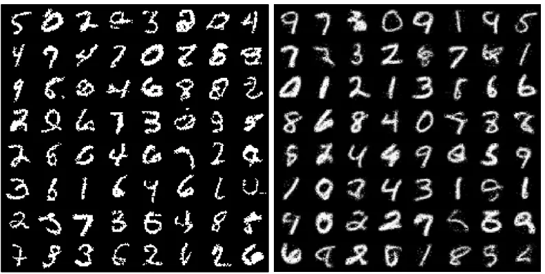
Pro-ceedings of the 25th Annual International Conference Figure 4: Left: samples from NADE trained on binarized MNIST. Right: probabilities
from which each pixel was sampled. Ancestral sampling was used with the same fixed ordering used during training.
Model −logp ≤
DRAW (without attention) 87.40
DRAW 80.97
Pixel RNN 79.20
ConvNADE+DeepNADE (no input masks) 85.25
ConvNADE 81.30
ConvNADE+DeepNADE 80.82
Table 4: Negative log-likelihood test results of models exploiting 2D topology on the binarized MNIST data set.
Now, addressing the second question, we can see from Table 4 that convolutions do improve the performance of NADE. Moreover, we observe that providing information about which inputs are masked is essential to obtaining good results. We can also see that combining convolutional and fully-connected layers helps. Even though ConvNADE+DeepNADE performs slightly worse than Pixel RNN, we note that our proposed approach is order-agnostic, whereas Pixel RNN requires a fixed ordering. Figure 7 shows samples obtained from the ConvNADE+DeepNADE model using ancestral sampling on a random ordering.
7.3 Real-Valued Observations Data Sets
In this section, we compare the statistical performance of RNADE to mixtures of Gaus-sians (MoG) and factor analyzers (MFA), which are surprisingly strong baselines in some tasks (Tang et al., 2012; Zoran and Weiss, 2012).
Image
64@8x8(valid)
64@4x4(valid)
64@6x6(valid)
64@7x7(valid)
64@4x4(full) 64@6x6(full) 64@7x7(full)
1@8x8(full)
Output
(a) ConvNADE
Image
64@8x8(valid)
64@4x4(valid)
64@6x6(valid)
64@7x7(valid)
64@4x4(full) 64@6x6(full) 64@7x7(full)
1@8x8(full)
Output
500
500
784
+
(b) ConvNADE + DeepNADE
-61.21 -36.33
-84.40 -46.22
-96.68 -66.26
-86.37 -73.31
-93.35 -79.40
-45.84 -41.88
Figure 6: Example of marginalization and sampling. The first column shows five examples from the test set of the MNIST data set. The second column shows the density of these examples when a random 10×10 pixel region is marginalized. The right-most five columns show samples for the hollowed region. Both tasks can be done easily with a NADE where the pixels to marginalize are at the end of the ordering.
0 50 100 150 200
0
50
100
150
200
Samples
7.3.1 Low-dimensional data
We start by considering three UCI data sets (Bache and Lichman, 2013), previously used to study the performance of other density estimators (Silva et al., 2011; Tang et al., 2012), namely: red wine, white wine and parkinsons. These are low dimensional data sets (see Table 5) with hard thresholds and non-linear dependencies that make it difficult to fit mixtures of Gaussians or factor analyzers.
Following Tang et al. (2012), we eliminated discrete-valued attributes and an attribute from every pair with a Pearson correlation coefficient greater than 0.98. We normalized each dimension of the data by subtracting its training-subset sample mean and dividing by its standard deviation. All results are reported on the normalized data.
We use full-covariance Gaussians and mixtures of factor analysers as baselines. Models were compared on their log-likelihood on held-out test data. Due to the small size of the data sets (see Table 5), we used 10-folds, using 90% of the data for training, and 10% for testing.
We chose the hyperparameter values for each model by doing per-fold cross-validation, using a ninth of the training data as validation data. Once the hyperparameter values have been chosen, we train each model using all the training data (including the validation data) and measure its performance on the 10% of held-out testing data. In order to avoid overfitting, we stopped the training after reaching a training likelihood higher than the one obtained on the best validation-wise iteration of the best validation run. Early stopping was important to avoid overfitting the RNADE models. It also improved the results of the MFAs, but to a lesser degree.
The MFA models were trained using the EM algorithm (Ghahramani and Hinton, 1996; Verbeek, 2005). We cross-validated the number of components and factors. We also selected the number of factors from 2,4, . . . D, where choosingDresults in a mixture of Gaussians, and the number of components was chosen among 2,4, . . .50. Cross-validation selected fewer than 50 components in every case.
We report the performance of several RNADE models using different parametric forms for the one-dimensional conditionals: Gaussian with fixed variance (RNADE-FV), Gaussian with variable variance (RNADE-Gaussian),sinh-arcsinh distribution (RNADE-SAS), mixture of Gaussians (RNADE-MoG), and mixture of Laplace distributions (RNADE-MoL). All RNADE models were trained by stochastic gradient descent, using minibatches of size 100, for 500 epochs, each epoch comprising 10 minibatches. We fixed the number of hidden units to 50, and the non-linear activation function of the hidden units to ReLU. Three hyperparameters were cross-validated using grid-search: the number of components on each one-dimensional conditional (only applicable to the RNADE-MoG and RNADE-MoL models) was chosen from {2,5,10,20}, the weight-decay (used only to regularize the input to hidden weights) from {2.0,1.0,0.1,0.01,0.001,0}, and the learning rate from {0.1,0.05,0.025,0.0125}. Learning rates were decreased linearly to reach 0 after the last epoch.
−20 0 20 40 60 80 x6
−50
0 50 100 150 200 250 300
x7
RNADE-FV
−20 0 20 40 60 80
x6
−50
0 50 100 150 200 250 300
x7
RNADE-Gaussian
−20 0 20 40 60 80
x6
−50
0 50 100 150 200 250 300
x7
RNADE-SAS
−20 0 20 40 60 80
x6
−50
0 50 100 150 200 250 300
x7
RNADE-MoG K=20
Figure 8: Scatter plot of dimensions x7 vs x6 of the red wine data set. A thousand data
points from the data set are shown in black in all subfigures. As can be observed, this conditional distribution p(x7|x6) is heteroscedastic, skewed and has hard
Red wine White wine Parkinsons
Dimensionality 11 11 15
Total number of data points 1599 4898 5875
Table 5: Dimensionality and size of the UCI data sets used in Section 7.3.1
Model Red wine White wine Parkinsons
Gaussian −13.18 −13.20 −10.85
MFA −10.19 −10.73 −1.99
RNADE-FV −12.29 −12.50 −8.87
RNADE-Gaussian −11.99 −12.20 −3.47
RNADE-SAS −9.86 −11.22 −3.07
RNADE-MoG −9.36 −10.23 −0.90
RNADE-MoL −9.46 −10.38 −2.63
Table 6: Average test set log-likelihoods per data point for seven models on three UCI data sets. Performances not in bold can be shown to be significantly worse than at least one of the results in bold as per a pairedt-test on the ten mean-likelihoods (obtained from each data fold), with significance level 0.05.
7.3.2 Natural image patches
We also measured the ability of RNADE to model small patches of natural images. Following the work of Zoran and Weiss (2011), we use 8-by-8-pixel patches of monochrome natural images, obtained from the BSDS300 data set (Martin et al., 2001; Figure 9 gives examples).
Pixels in this data set can take a finite number of brightness values ranging from 0 to 255. We added uniformly distributed noise between 0 and 1 to the brightness of each pixel. We then divided by 256, making the pixels take continuous values in the range [0,1]. Adding noise prevents deceivingly high-likelihood solutions that assign narrow high-density spikes around some of the possible discrete values.
We subtracted the mean pixel value from each patch. Effectively reducing the dimen-sionality of the data. Therefore we discarded the 64th (bottom-right) pixel, which would be perfectly predictable and models could fit arbitrarily high densities to it. All of the results in this section were obtained by fitting the pixels in a raster-scan order.
All RNADE models reported use ReLU activations for the hidden units. The RNADE models were trained by stochastic gradient descent, using 25 data points per minibatch, for a total of 1,000 epochs, each comprising 1,000 minibatches. The learning rate was initialized to 0.001, and linearly decreased to reach 0 after the last epoch. Gradient momentum with factor 0.9 was used, but initiated after the first epoch. A weight decay rate of 0.001 was applied to the input-to-hidden weight matrix only. We found that multiplying the gradient of the mean output parameters by the standard deviation improves results of the models with mixture outputs5. RNADE training was early stopped but didn’t show signs of overfitting. Even larger models might perform better.
The MoG models were trained using 1,000 iterations of minibatch EM. At each iteration 20,000 randomly sampled data points were used in an EM update. A step was taken from the previous parameters’ value towards the parameters resulting from the M-step:
θt = (1−η)θt−1+ηθEM. The step size, η, was scheduled to start at 0.1 and linearly
decreased to reach 0 after the last update. The training of the MoG was early-stopped and also showed no signs of overfitting.
The results are shown in Table 7. We report the average log-likelihood of each model for a million image patches from the test set. The ranking of RNADE models is maintained when ordered by validation likelihood: the model with best test-likelihood would have been chosen using crossvalidation across all the RNADE models shown in the table. We also compared RNADE with a MoG trained by Zoran and Weiss (downloaded from Daniel Zoran’s website) from which we removed the 64th row and column of each covariance matrix. There are two differences in the set-up of our experiments and those of Zoran and Weiss. First, we learned the means of the MoG components, while Zoran and Weiss (2011) fixed them to zero. Second, we held-out 20 images from the training set to do early-stopping and hyperparameter optimisation, while they used the 200 images for training.
The RNADE-FV model with fixed conditional variances obtained very low statistical performance. Adding an output parameter per dimension to have variable standard deviations made our models competitive with MoG with 100 full-covariance components. However, in order to obtain results superior to the mixture of Gaussians model trained by Zoran and Weiss, we had to use richer conditional distributions: one-dimensional mixtures of Gaussians (RNADE-MoG). On average, the best RNADE model obtained 3.3 nats per patch higher
log-density than a MoG fitted with the same training data.
In Figure 9, we show one hundred examples from the test set, one hundred examples from Zoran and Weiss’ mixture of Gaussians, and a hundred samples from our best RNADE-MoG model. Similar patterns can be observed in the three cases: uniform patches, edges, and locally smooth noisy patches.
7.3.3 Speech acoustics
We also measured the ability of RNADE to model small patches of speech spectrograms, extracted from the TIMIT data set (Garofolo et al., 1993). The patches contained 11 frames of 20 filter-banks plus energy; totalling 231 dimensions per data point. A good generative model of speech acoustics could be used, for example, in denoising, or speech detection tasks.
Model Test log-likelihood
MoGK= 200 (Zoran and Weiss, 2012)a 152.8
MoGK= 100 144.7
MoGK= 200 150.4
MoGK= 300 150.4
RNADE-FVh= 512 100.3
RNADE-Gaussianh= 512 143.9
RNADE-Laplace h= 512 145.9
RNADE-SASb h= 512 148.5
RNADE-MoGK= 2h= 512 149.5
RNADE-MoGK= 2h= 1024 150.3
RNADE-MoGK= 5h= 512 152.4
RNADE-MoGK= 5h= 1024 152.7
RNADE-MoGK= 10h= 512 153.5
RNADE-MoGK= 10h= 1024 153.7
RNADE-MoLK= 2h= 512 149.3
RNADE-MoLK= 2h= 1024 150.1
RNADE-MoLK= 5h= 512 151.5
RNADE-MoLK= 5h= 1024 151.4
RNADE-MoLK= 10 h= 512 152.3
RNADE-MoLK= 10 h= 1024 152.5
Table 7: Average per-example log-likelihood of several mixture of Gaussian and RNADE models on 8×8 pixel patches of natural images. These results are reported in nats and were calculated using one million patches. Standard errors due to the finite test sample size are lower than 0.1 nats in every case. hindicates the number of hidden units in the RNADE models, andKthe number of one-dimensional components for each conditional in RNADE or the number of full-covariance components for MoG.
a. This model was trained using the full 200 images in the BSDS training data set, the rest of the models were trained using 180, reserving 20 for hyperparameter crossvalidation and early-stopping.
Model Test LogL
MoG N= 50 110.4
MoG N= 100 112.0
MoG N= 200 112.5
MoG N= 300 112.5
RNADE-Gaussian 110.6
RNADE-Laplace 108.6
RNADE-SAS 119.2
RNADE-MoGK= 2 121.1
RNADE-MoGK= 5 124.3
RNADE-MoGK= 10 127.8
RNADE-MoL K= 2 116.3
RNADE-MoL K= 5 120.5
RNADE-MoL K= 10 123.3
Table 8: Log-likelihood of several MoG and RNADE models on the core-test set of TIMIT measured in nats. Standard errors due to the finite test sample size are lower than 0.4 nats in every case. RNADE obtained a higher (better) log-likelihood.
We fitted the models using the standard TIMIT training subset, which includes recordings from 605 speakers of American English. We compare RNADE with a mixture of Gaussians by measuring their log-likelihood on the complete TIMIT core-test data set: a held-out set of 25 speakers.
The RNADE models have 512 hidden units, ReLU activations, and a mixture of 20 one-dimensional Gaussian components per output. Given the large scale of this data set, hyperparameter choices were again made manually using validation data. The same training procedures for RNADE and mixture of Gaussians were used as for natural image patches.
The RNADE models were trained by stochastic gradient descent, with 25 data points per minibatch, for a total of 200 epochs, each comprising 1,000 minibatches. The learning rate was initialized to 0.001 and linearly decreased to reach 0 after the last epoch. Gradient momentum with momentum factor 0.9 was used, but initiated after the first epoch. A weight decay rate of 0.001 was applied to the input-to-hidden weight matrix only. Again, we found that multiplying the gradient of the mean output parameters by the standard deviation improved results. RNADE training was early stopped but didn’t show signs of overfitting.
As for the MoG model, it was trained exactly as in Section 7.3.2.
8. Conclusion
We’ve described the Neural Autoregressive Distribution Estimator, a tractable, flexible and competitive alternative to directed and undirected graphical models for unsupervised distribution estimation.
Since the publication of the first formulation of NADE (Larochelle and Murray, 2011), it has been extended to many more settings, other than those described in this paper. Larochelle and Lauly (2012); Zheng et al. (2015b) adapted NADE for topic modeling of documents and images, while Boulanger-Lewandowski et al. (2012) used NADE for modeling music sequential data. Theis and Bethge (2015) and Oord et al. (2016) proposed different NADE models for images than the one we presented, applied to natural images and based on convolutional and LSTM hidden units. Zheng et al. (2015a) used a NADE model to integrate an attention mechanism into an image classifier. Bornschein and Bengio (2015) showed that NADE could serve as a powerful prior over the latent state of directed graphical model. These are just a few examples of many possible ways one can leverage the flexibility and effectiveness of NADE models.
References
Kevin Bache and Moshe Lichman. UCI machine learning repository, 2013. http://archive. ics.uci.edu/ml.
Yoshua Bengio. Learning deep architectures for AI. Foundations and Trends in Machine Learning, 2(1):1–127, 2009.
Yoshua Bengio and Samy Bengio. Modeling high-dimensional discrete data with multi-layer neural networks. InAdvances in Neural Information Processing Systems 12, pages 400–406. MIT Press, 2000.
Julian Besag. Statistical analysis of non-lattice data. The Statistician, 24(3):179–195, 1975.
Christopher M. Bishop. Mixture density networks. Technical Report NCRG 4288, Neural Computing Research Group, Aston University, Birmingham, 1994.
J¨org Bornschein and Yoshua Bengio. Reweighted wake-sleep. In Proceedings of the 3rd International Conference on Learning Representations. arXiv:1406.2751, 2015.
Nicolas Boulanger-Lewandowski, Yoshua Bengio, and Pascal Vincent. Modeling temporal dependencies in high-dimensional sequences: Application to polyphonic music generation and transcription. In Proceedings of the 29th International Conference on Machine Learning, pages 1159–1166. Omnipress, 2012.
Yuri Burda, Ruslan Salakhutdinov, and Roger Grosse. Importance weighted autoen-coders. In Proceedings of the 4th International Conference on Learning Representations. arXiv:1509.00519v3, 2016.