Information Bottleneck for Gaussian Variables
Gal Chechik∗ [email protected]
Computer Science Department Stanford University
Stanford CA 94305-9025, USA
Amir Globerson∗ [email protected]
Naftali Tishby [email protected]
Yair Weiss [email protected]
School of Computer Science and Engineering and The Interdisciplinary Center for Neural Computation The Hebrew University of Jerusalem
Givat Ram, Jerusalem 91904, Israel
Editor: Peter Dayan
Abstract
The problem of extracting the relevant aspects of data was previously addressed through the
infor-mation bottleneck (IB) method, through (soft) clustering one variable while preserving inforinfor-mation
about another - relevance - variable. The current work extends these ideas to obtain continuous rep-resentations that preserve relevant information, rather than discrete clusters, for the special case of multivariate Gaussian variables. While the general continuous IB problem is difficult to solve, we provide an analytic solution for the optimal representation and tradeoff between compression and relevance for the this important case. The obtained optimal representation is a noisy linear projec-tion to eigenvectors of the normalized regression matrixΣx|yΣ−x1, which is also the basis obtained in canonical correlation analysis. However, in Gaussian IB, the compression tradeoff parameter uniquely determines the dimension, as well as the scale of each eigenvector, through a cascade of structural phase transitions. This introduces a novel interpretation where solutions of different ranks lie on a continuum parametrized by the compression level. Our analysis also provides a complete analytic expression of the preserved information as a function of the compression (the “information-curve”), in terms of the eigenvalue spectrum of the data. As in the discrete case, the information curve is concave and smooth, though it is made of different analytic segments for each optimal dimension. Finally, we show how the algorithmic theory developed in the IB framework provides an iterative algorithm for obtaining the optimal Gaussian projections.
Keywords: information bottleneck, Gaussian processes, dimensionality reduction, canonical
cor-relation analysis
1. Introduction
Extracting relevant aspects of complex data is a fundamental task in machine learning and statistics. The problem is often that the data contains many structures, which make it difficult to define which of them are relevant and which are not in an unsupervised manner. For example, speech signals may
be characterized by their volume level, pitch, or content; pictures can be ranked by their luminosity level, color saturation or importance with regard to some task.
This problem was addressed in a principled manner by the information bottleneck (IB) approach (Tishby et al., 1999). Given the joint distribution of a “source” variable X and another “relevance” variable Y , IB operates to compress X , while preserving information about Y . The variable Y thus implicitly defines what is relevant in X and what is not. Formally, this is cast as the following variational problem
min
p(t|x)
L
:L
≡I(X ; T)−βI(T ;Y) (1)where T represents the compressed representation of X via the conditional distributions p(t|x), while the information that T maintains on Y is captured by the distribution p(y|t). This formulation is general and does not depend on the type of the X,Y distribution. The positive parameter β
determines the tradeoff between compression and preserved relevant information, as the Lagrange multiplier for the constrained optimization problem minp(t|x)I(X ; T)−β(I(T ;Y)−const). Since T
is a function of X it is independent of Y given X , thus the three variables can be written as the Markov chain Y−X−T . From the information inequality we thus have I(X ; T)−βI(T ;Y)≥(1−β)I(T ;Y), and therefore for all values ofβ≤1, the optimal solution of the minimization problem is degenerated
I(T ; X) =I(T ;Y) =0. As we will show below, the range of degenerated solutions is even larger for
Gaussian variables and depends on the eigen spectrum of the variables covariance matrices. The rationale behind the IB principle can be viewed as model-free “looking inside the black-box” system analysis approach. Given the input-output (X,Y) “black-box” statistics, IB aims to construct efficient representations of X , denoted by the variable T , that can account for the observed statistics of Y . IB achieves this using a single tradeoff parameter to represent the tradeoff between the complexity of the representation of X , measured by I(X ; T), and the accuracy of this representa-tion, measured by I(T ;Y). The choice of mutual information for the characterization of complexity and accuracy stems from Shannon’s theory, where information minimization corresponds to optimal compression in Rate Distortion Theory, and its maximization corresponds to optimal information transmission in Noisy Channel Coding.
From a machine learning perspective, IB may be interpreted as regularized generative modeling. Under certain conditions I(T ;Y)can be interpreted as an empirical likelihood of a special mixture model, and I(T ; X)as penalizing complex models (Slonim and Weiss, 2002). While this interpreta-tion can lead to interesting analogies , it is important to emphasize the differences. First, IB views
I(X ; T)not as a regularization term, but rather corresponds to the distortion constraint in the
origi-nal system. As a result, this constraint is useful even when the joint distribution is known exactly, because the goal of IB is to obtain compact representations rather than to estimate density. Inter-estingly, I(T ; X)also characterizes the complexity of the representation T as the expected number of bits needed to specify the t for a given x. In that role it can be viewed as an expected “cost” of the internal representation, as in MDL. As is well acknowledged now source coding with distortion and channel coding with cost are dual problems (see for example Shannon, 1959; Pradhan et al., 2003). In that information theoretic sense, IB is self dual, where the resulting source and channel are perfectly matched (as in Gastpar and Vetterli, 2003).
and Miller, 2001) to gene expression analysis (Friedman et al., 2001; Sinkkonen and Kaski, 2001) (for a more detailed review of IB clustering algorithms see Slonim (2003)). However, its general information theoretic formulation is not restricted, both in terms of the nature of the variables X and Y , as well as of the compression variable T . It can be naturally extended to nominal, categorical, and continuous variables, as well as to dimension reduction rather than clustering techniques. The goal of this paper is apply the IB for the special, but very important, case of Gaussian processes which has become one of the most important generative classes in machine learning. In addition, this is the first concrete application of IB to dimension reduction with continuous compressed representation, and as such exhibit interesting dimension related phase transitions.
The general solution of IB for continuous T yields the same set of self-consistent equations obtained already in (Tishby et al., 1999), but solving these equations for the distributions p(t|x), p(t)
and p(y|t) without any further assumptions is a difficult challenge, as it yields non-linear coupled eigenvalue problems. As in many other cases, however, we show here that the problem turns out to be analytically tractable when X and Y are joint multivariate Gaussian variables. In this case, rather than using the fixed point equations and the generalized Blahut-Arimoto algorithm as proposed in (Tishby et al., 1999), one can explicitly optimize the target function with respect to the mapping p(t|x)and obtain a closed form solution of the optimal dimensionality reduction.
The optimal compression in the Gaussian information bottleneck (GIB) is defined in terms of the compression-relevance tradeoff (also known as the “Information Curve”, or “Accuracy-Complexity” tradeoff), determined by varying the parameterβ. The optimal solution turns out to be a noisy linear projection to a subspace whose dimensionality is determined by the parameterβ. The subspaces are spanned by the basis vectors obtained as in the well known canonical correlation analysis (CCA) (Hotelling, 1935), but the exact nature of the projection is determined in a unique way via the parameterβ. Specifically, asβincreases, additional dimensions are added to the projection variable T , through a series of critical points (structural phase transitions), while at the same time the relative magnitude of each basis vector is rescaled. This process continues until all the relevant information about Y is captured in T . This demonstrates how the IB principle can provide a continuous measure of model complexity in information theoretic terms.
The idea of maximization of relevant information was also taken in the Imax framework of Becker and Hinton (Becker and Hinton, 1992; Becker, 1996), which followed Linsker’s idea of information maximization (Linsker, 1988, 1992). In the Imax setting, there are two one-layer feed forward networks with inputs Xa, Xb and outputs neurons Ya, Yb; the output neuron Ya serves to define relevance to the output of the neighboring network Yb. Formally, the goal is to tune the incoming weights of the output neurons, such that their mutual information I(Ya;Yb)is maximized. An important difference between Imax and the IB setting, is that in the Imax setting, I(Ya;Yb) is invariant to scaling and translation of the Y ’s since the compression achieved in the mapping Xa→Ya is not modeled explicitly. In contrast, the IB framework aims to characterize the dependence of the solution on the explicit compression term I(T ; X), which is a scale sensitive measure when the transformation is noisy. This view of compressed representation T of the inputs X is useful when dealing with neural systems that are stochastic in nature and limited in their responses amplitudes and are thus constrained to finite I(T ; X).
algorithm can be adapted to the Gaussian case, yielding an iterative algorithm for finding the optimal projections. The relations to canonical correlation analysis and coding with side-information are discussed in Section 9.
2. Gaussian Information Bottleneck
We now formalize the problem of information bottleneck for Gaussian variables. Let(X,Y)be two jointly multivariate Gaussian variables of dimensions nx, ny and denote byΣx,Σy the covariance matrices of X ,Y and byΣxytheir cross-covariance matrix.1The goal of GIB is to compress the vari-able X via a stochastic transformation into another varivari-able T ∈Rnx, while preserving information
about Y . The dimension of T is not explicitly limited in our formalism, since we will show that the effective dimension is determined by the value ofβ.
It is shown in Globerson and Tishby (2004) that the optimum for this problem is obtained by a variable T which is also jointly Gaussian with X . The formal proof uses the entropy power inequality as in Berger and Zamir (1999), and is rather technical, but an intuitive explanation is that since X and Y are Gaussians, the only statistical dependencies that connect them are bi-linear. Therefore, a linear projection of X is sufficient to capture all the information that X has on Y . The Entropy-power inequality is used to show that a linear projection of X , which is also Gaussian in this case, indeed attains this maximum information.
Since every two centered random variables X and T with jointly Gaussian distribution can be presented through the linear transformation T=AX+ξ, whereξ∼N(0,Σξ)is another Gaussian that
is independent of X , we formalize the problem using this representation of T , as the minimization
min A,Σξ
L
≡I(X ; T)−βI(T ;Y) (2)over the noisy linear transformations of A,Σξ
T=AX+ξ; ξ∼N(0,Σξ). (3)
Thus T is normally distributed T ∼N(0,Σt)withΣt =AΣxAT+Σξ.
Interestingly, the term ξ can also be viewed as an additive noise term, as commonly done in models of learning in neural networks. Under this view, ξserves as a regularization term whose covariance determines the scales of the problem. While the goal of GIB is to find the optimal projection parameters A,Σξjointly, we show below that the problem factorizes such that the optimal projection A does not depend on the noise, which does not carry any information about Y .
3. The Optimal Projection
The first main result of this paper is the characterization of the optimal A,Σξas a function ofβ
1. For simplicity we assume that X and Y have zero means andΣx,Σyare full rank. Otherwise X and Y can be centered
Theorem 3.1 The optimal projection T =AX+ξ for a given tradeoff parameter β is given by
Σξ=Ix and
A=
0T;. . .; 0T 0≤β≤βc1
α
1vT1,0T;. . .; 0T
βc
1≤β≤βc2
α1vT1;α2vT2; 0T;. . .; 0T
βc
2≤β≤βc3 ..
.
(4)
where {vT1,vT2, . . . ,vnTx} are left eigenvectors of Σx|yΣ−x1 sorted by their corresponding ascending eigenvalues λ1,λ2, . . . ,λnx, β
c
i = 1−λ1 i are critical β values, αi are coefficients defined by αi ≡
q
β(1−λi)−1
λiri , ri ≡v
T
i Σxvi, 0T is an nx dimensional row vector of zeros, and semicolons separate
rows in the matrix A.
This theorem asserts that the optimal projection consists of eigenvectors ofΣx|yΣ−1
x , combined in an interesting manner: Forβvalues that are smaller than the smallest critical pointβc1, compression is more important than any information preservation and the optimal solution is the degenerated one A≡0. As βis increased, it goes through a series of critical points βc
i, at each of which another eigenvector ofΣx|yΣ−x1is added to A. Even though the rank of A increases at each of these transition points, A changes continuously as a function ofβsince at each critical pointβci the coefficient αi vanishes. Thusβparameterizes a sort of “continuous rank” of the projection.
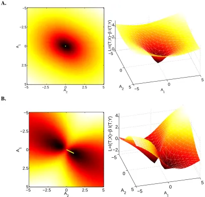
To illustrate the form of the solution, we plot the landscape of the target function
L
together with the solution in a simple problem where X∈R2and Y∈R. In this case A has a single non-zero row, thus A can be thought of as a row vector of length 2, that projects X to a scalar A : X →R,T∈R. Figure 1 shows the target function
L
as a function of the (vector of length 2) projection A. Inthis example, the largest eigenvalue isλ1=0.95, yieldingβc1=20. Therefore, forβ=15 (Figure 1A) the zero solution is optimal, but forβ=100>βc (Figure 1B) the corresponding eigenvector is a feasible solution, and the target function manifold contains two mirror minima. Asβincreases from 1 to∞, these two minima, starting as a single unified minimum at zero, split atβc, and then diverge apart to∞.
We now turn to prove Theorem 3.1.
4. Deriving the Optimal Projection
We first rewrite the target function as
L
=I(X ; T)−βI(T ;Y) =h(T)−h(T|X)−βh(T) +βh(T|Y) (5)where h is the (differential) entropy of a continuous variable
h(X)≡ − Z
X
f(x)log f(x)dx.
Recall that the entropy of a d dimensional Gaussian variable is
h(X) =1
2log
(2πe)d|Σx|
A.
A1
A2
−5 −2.5 0 2.5 5
−5
−2.5
0
2.5
5
−5
0
5 −5 0
5 0
2 4
A
1
A
2
L=I(T;X)−
β
I(T;Y)
B.
A 1
A2
−5 −2.5 0 2.5 5 −5
−2.5
0
2.5
5
−5
0
5 −5 0
5 −2
0 2 4
A1
A
2
L=I(T;X)−
β
I(T;Y)
where|x|denotes the determinant of x, andΣxis the covariance of X . We therefore turn to calcu-late the relevant covariance matrices. From the definition of T we haveΣtx =AΣx,Σty=AΣxyand
Σt =AΣxAT+Σξ. Now, the conditional covariance matrixΣx|ycan be used to calculate the covari-ance of the conditional variable T|Y , using the Schur complement formula (see e.g., Magnus and Neudecker, 1988)
Σt|y=Σt−ΣtyΣ−y1Σyt =AΣx|yAT+Σξ. The target function can now be rewritten as
L
= log(|Σt|)−log(|Σt|x|)−βlog(|Σt|) +βlog(|Σt|y|). (6)= (1−β)log(|AΣxAT+Σξ|)−log(|Σξ|) +βlog(|AΣx|yAT+Σξ|)
Although
L
is a function of both the noiseΣξand the projection A, Lemma A.1 in Appendix A shows that for every pair (A,Σξ), there is another projection ˜A such that the pair (A˜,I) obtains the same value ofL
. This is obtained by setting ˜A=√D−1VA where Σξ=V DVT, which yields
L
(A˜,I) =L
(A,Σξ).2 This allows us to simplify the calculations by replacing the noise covariance matrixΣξwith the identity matrix Id.To identify the minimum of
L
we differentiateL
with respect to the projection A using the algebraic identity δδAlog(|ACAT|) = (ACAT)−12AC which holds for any symmetric matrix C:δ
L
δA = (1−β)(AΣxA T+I
d)−12AΣx+β(AΣx|yAT+Id)−12AΣx|y. (7) Equating this derivative to zero and rearranging, we obtain necessary conditions for an internal minimum of
L
, which we explore in the next two sections.4.1 Scalar Projections
For clearer presentation of the general derivation, we begin with a sketch of the proof by focusing on the case where T is a scalar, that is, the optimal projection matrix A is a now a single row vector. In this case, both AΣxAT and AΣx|yAT are scalars, and we can write
β
−1
β
AΣ
x|yAT+1 AΣxAT+1
!
A=AΣ
x|yΣ−x1
. (8)
This equation is therefore an eigenvalue problem in which the eigenvalues depend on A. It has two types of solutions depending on the value ofβ. First, A may be identically zero. Otherwise, A must
be the eigenvector ofΣx|yΣ−x1, with an eigenvalueλ= β− 1
β
AΣx|yAT+1
AΣxAT+1
To characterize the values ofβfor which the optimal solution does not degenerate, we find when the eigenvector solution is optimal. Denote the norm ofΣx with respect to A by r=AΣxA
T
||A||2 . When A
is an eigenvector ofΣx|yΣ−x1, Lemma B.1 shows that r is positive and that AΣx|yΣx−1ΣxAT=λr||A||2. Rewriting the eigenvalue and isolating||A||2, we have
0<||A||2=β(1−λ)−1
rλ . (9)
A. B.
1 10 100 1000
0 0.2 0.4 0.6 0.8 1
Feasible region
β
λ
1
10
100
0 0.5
1 0 5 10
β λ
log(||A||
2)
Figure 2: A. The regions of (β,λ) pairs that lead to the zero (red) and eigenvector (blue) solutions. B. The norm||A||2as a function ofβandλover the feasible region.
This inequality provides a constraint on β and λ that is required for a non-degenerated type of solution
λ≤β−β1 or β≥(1−λ)−1, (10)
thus defining a critical value βc(λ) = (1−λ)−1. For β≤βc(λ), the weight of compression is so strong that the solution degenerates to zero and no information is carried about X or Y . For
β≥βc(λ)the weight of information preservation is large enough, and the optimal solution for A is an eigenvector ofΣx|yΣ−x1. The feasible regions for non degenerated solutions and the norm||A||2 as a function ofβandλare depicted in Figure 2.
For someβvalues, several eigenvectors can satisfy the condition for non degenerated solutions of Equation (10). Appendix C shows that the optimum is achieved by the eigenvector ofΣx|yΣ−x1 with the smallest eigenvalue. Note that this is also the eigenvector ofΣxyΣ−y1ΣyxΣ−x1with the largest eigenvalue. We conclude that for scalar projections
A(β) =
q
β(1−λ)−1
rλ v1 0<λ≤
β−1
β
0 β−β1 ≤λ≤1 (11)
where v1is the eigenvector ofΣx|yΣ−x1with the smallest eigenvalue.
4.2 The High-Dimensional Case
We now return to the proof of the general, high dimensional case, which follows the same lines as the scalar projection case. Setting the gradient in Equation (7) to zero and reordering we obtain
β−1
β
(AΣx|yAT+Id)(AΣxAT+Id)−1
A=AΣx|yΣ−x1
. (12)
represent the projection A as a mixture A=WV where the rows of V are left normalized eigenvectors ofΣx|yΣ−x1and W is a mixing matrix that weights these eigenvectors. The form of the mixing matrix W , that characterizes the norms of these eigenvectors, is described in the following lemma, which is proved in Appendix D.
Lemma 4.1 The optimum of the cost function is obtained with a diagonal mixing matrix W of the form
W=diag
s
β(1−λ1)−1
λ1r1
, . . . , s
β(1−λk)−1
λkrk
,0, . . . ,0
(13)
where{λ1, . . . ,λk} are k≤nx eigenvalues ofΣx|yΣx−1 with criticalβvaluesβc1, . . . ,βck ≤β. ri≡
vTi Σxvias in Theorem 3.1.
The proof is presented in Appendix D.
We have thus characterized the set of all minima of
L
, and turn to identify which of them achieve the global minima.Corollary 4.2
The global minimum of
L
is obtained with allλithat satisfyλi<β−β1.The proof is presented in Appendix D.
Taken together, these observations prove that for a given value of β, the optimal projection is obtained by taking all the eigenvectors whose eigenvaluesλisatisfyβ≥1−λ1
i, and setting their norm
according to A=WV with W determined as in Lemma 4.1. This completes the proof of Theorem 3.1.
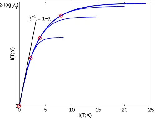
5. The GIB Information Curve
0 5 10 15 20 25 0
I(T;X)
I(T;Y)
Σ log(λi)
β−1
= 1−λ
1
Figure 3: GIB information curve obtained with four eigenvaluesλi=0.1,0.5,0.7,0.9. The informa-tion at the critical points are designated by circles. For infiniteβ, curve is saturated at the log of the determinant∑logλi. For comparison, information curves calculated with smaller number of eigenvectors are also depicted (all curves calculated forβ<1000). The slope of the un-normalized curve at each point is the correspondingβ−1. The tangent at zero, with slopeβ−1=1−λ
1, is super imposed on the information curve.
To this end, we substitute the optimal projection A(β)into I(T ; X)and I(T ;Y)and rewrite them as a function ofβ
Iβ(T ; X) = 1
2log |AΣxA T+I
d|
(14)
= 1
2log |(β(I−D)−I)D
−1 |
= 1
2 n(β)
∑
i=1 log
(β−1)1−λi
λi
Iβ(T ;Y) = I(T ; X)−1
2 n(β)
∑
i=1
logβ(1−λi),
where D is a diagonal matrix whose entries are the eigenvalues ofΣx|yΣ−x1 as in Appendix D, and n(β)is the maximal index i such thatβ≥1−λ1
i. Isolatingβas a function of Iβ(T ; X)in the correct
range of nβand then Iβ(T ;Y)as a function of Iβ(T ; X)we have
I(T ;Y) =I(T ; X)−nI
2 log nI
∏
i=1
(1−λi)
1 nI +e
2I(T ;X)
nI
nI
∏
i=1
λi
1 nI
!
(15)
where the products are over the first nI =nβ(I(T ;X)) eigenvalues, since these obey the critical β
condition, with cnI ≤I(T ; X)≤cnI+1and cnI=∑
nI−1
i=1 log
λnI
λi
1−λi
The GIB curve, illustrated in Figure 3, is continuous and smooth, but is built of several seg-ments: as I(T ; X)increases additional eigenvectors are used in the projection. The derivative of the curve, which is equal to β−1, can be easily shown to be continuous and decreasing, therefore the information curve is concave everywhere, in agreement with the general concavity of information curve in the discrete case (Wyner, 1975; Gilad-Bachrach et al., 2003). Unlike the discrete case where concavity proofs rely on the ability to use a large number of clusters, concavity is guaranteed here also for segments of the curve, where the number of eigenvectors are limited a-priori.
At each value of I(T ; X)the curve is bounded by a tangent with a slopeβ−1(I(T ; X)). Generally in IB, the data processing inequality yields an upper bound on the slope at the origin,β−1(0)<1,
in GIB we obtain a tighter bound: β−1(0)<1−λ1. The asymptotic slope of the curve is always zero, as β→∞, reflecting the law of diminishing return: adding more bits to the description of X does not provide higher accuracy about T . This relation between the spectral properties of the covariance matrices raises interesting questions for special cases where the spectrum can be better characterized, such as random-walks and self-similar processes.
6. An Iterative Algorithm
The GIB solution is a set of scaled eigenvectors, and as such can be calculated using standard tech-niques. For example gradient ascent methods were suggested for learning CCA (Becker, 1996; Borga et al., 1997). An alternative approach is to use the general iterative algorithm for IB prob-lems (Tishby et al., 1999). This algorithm that can be extended to continuous variables and repre-sentations, but its practical application for arbitrary distributions leads to a non-linear generalized eigenvalue problem whose general solution can be difficult. It is therefore interesting to explore the form that the iterative algorithm assumes once it is applied to Gaussian variables. Moreover, it may be possible to later extend this approach to more general parametric distributions, such as general exponential forms, for which linear eigenvector methods may no longer be adequate.
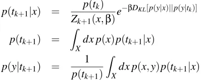
The general conditions for the IB stationary points were presented by Tishby et al. (1999) and can be written for a continuous variable x by the following self consistent equations for the unknown distributions p(t|x), p(y|t)and p(t):
p(t) = Z
X
dx p(x)p(t|x) (16)
p(y|t) = 1
p(t) Z
X
dx p(x,y)p(t|x)
p(t|x) = p(t)
Z(β)e
−βDKL[p(y|x)||p(y|t)]
equations can be iterated directly in a Blahut-Arimoto like algorithm,
p(tk+1|x) =
p(tk) Zk+1(x,β)
e−βDKL[p(y|x)||p(y|tk)] (17)
p(tk+1) =
Z
Xdx p
(x)p(tk+1|x) p(y|tk+1) =
1 p(tk+1)
Z
X
dx p(x,y)p(tk+1|x).
where each iteration results in a distribution over the variables Tk, X and Y . The second and third equations calculate p(tk+1)and p(y|tk+1)using standard marginalization, and the Markov property Y−X−Tk. These iterations were shown to converge to the optimal T by Tishby et al. (1999).
For the general continuous T such an iterative algorithm is clearly not feasible. We show here, how the fact that we are confined to Gaussian distributions, can be used to turn those equations into an efficient parameter updating algorithm. We conjecture that algorithms for parameters optimiza-tions can be defined also for parametric distribution other than Gaussians, such as other exponential distributions that can be efficiently represented with a small number of parameters.
In the case of Gaussian p(x,y), when p(tk|x)is Gaussian for some k, so are p(tk),p(y|tk)and p(tk+1|x). In other words, the set of Gaussians p(t|x)is invariant under the above iterations. To see why this is true, notice that p(y|tk)is Gaussian since Tkis jointly Gaussian with X . Also, p(tk+1|x) is Gaussian since DKL[p(y|x)||p(y|tk)]between two Gaussians contains only second order moments in y and t and thus its exponential is Gaussian. This is in agreement with the general fact that the optima (which are fixed points of 17) are Gaussian (Globerson and Tishby, 2004). This invariance allows us to turn the IB algorithm that iterates over distributions, into an algorithm that iterates over the parameters of the distributions, being the relevant degrees of freedom in the problem.
Denote the variable T at time k by Tk =AkX+ξk, where ξk∼
N
(0,Σξk). The parameters AandΣat time k+1 can be obtained by substituting Tk in the iterative IB equations. As shown in Appendix E, this yields the following update equations
Σξk+1 = βΣ−1
tk|y−(β−1)Σ
−1 tk
−1
(18)
Ak+1 = βΣξk+1Σ −1
tk|yAk I−Σy|xΣ
−1 x
whereΣtk|y,Σtk are the covariance matrices calculated for the variable Tk.
This algorithm can be interpreted as repeated projection of Akon the matrix I −Σy|xΣ−x1(whose eigenvectors we seek) followed by scaling withβΣξk+1Σt−1
k|y. It thus has similar form to the power
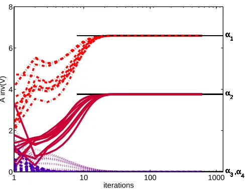
method for calculating the dominant eigenvectors of the matrixΣy|xΣ−x1(Demmel, 1997; Golub and Loan, 1989). However, unlike the naive power method, where only the single dominant eigenvector is preserved, the GIB iterative algorithm maintains several different eigenvectors, and their number is determined by the continuous parameter β and emerges from the iterations: All eigenvectors whose eigenvalues are smaller than the criticalβvanish to zero, while the rest are properly scaled. This is similar to an extension of the naive power method known as Orthogonal Iteration, in which the projected vectors are renormalized to maintain several non vanishing vectors (Jennings and Stewart, 1975).
1 10 100 1000 0 2 4 6 8 α1 α2
α3,α
4
iterations
A inv(V)
α1
α2
α3,α
4 α1
α2
α3,α
4 α1
α2
α3,α
4 α1
α2
α3,α
4 α1
α2
α3,α
4 α1
α2
α3,α
4 α1
α2
α3,α
4 α1
α2
α3,α
4 α1
α2
α3,α
4
Figure 4: The norm of projection on the four eigenvectors ofΣx|yΣ−1
x , as evolves along the operation of the iterative algorithm. Each line corresponds to the length of the projection of one row of A on the closest eigenvector. The projection on the other eigenvectors also vanishes (not shown). β was set to a value that leads to two non vanishing eigenvectors. The algorithm was repeated 10 times with different random initialization points, showing that it converges within 20 steps to the correct valuesαi.
The iterative algorithm can also be interpreted as a regression of X on T via Y . This can be seen by writing the update equation for Ak+1as
Ak+1=Σξk+1Σ −1 tk|y ΣytkΣ
−1 y
Σ
yxΣ−x1
. (19)
SinceΣyxΣ−x1 describes the optimal linear regressor of X on Y , the operation of Ak+1on X can be described by the following diagram
X ΣyxΣ
−1 x
−−−−→µy|x
ΣytkΣ−1 y
−−−−→µtk|µy|x
Σξk+1Σ −1 tk|y
−−−−−→Tk+1 (20)
where the last step scales and normalizes T .
7. Relation To Other Works
The GIB solutions are related to studies of two main types: studies of eigenvalues based co-projections, and information theoretic studies of continuous compression. We review both below.
7.1 Canonical Correlation Analysis and Imax
finds linear relations between two variables. Given two variables X,Y , CCA finds a set of basis vec-tors for each variable, such that the correlation coefficient between the projection of the variables on the basis vectors is maximized. In other words, it finds the bases in which the correlation matrix is diagonal and the correlations on the diagonal are maximized. The bases are the eigenvectors of the matricesΣ−y1ΣyxΣ−x1ΣxyandΣ−x1ΣxyΣ−y1Σyx, and the square roots of their corresponding eigenvalues are the canonical correlation coefficients. CCA was also shown to be a special case of continu-ous Imax (Becker and Hinton, 1992; Becker, 1996), when the Imax networks are limited to linear projections.
Although GIB and CCA involve the spectral analysis of the same matrices, they have some inherent differences. First of all, GIB characterizes not only the eigenvectors but also their norm, in a way that that depends on the trade-off parameter β. Since CCA depends on the correlation coefficient between the compressed (projected) versions of X and Y , which is a normalized measure of correlation, it is invariant to a rescaling of the projection vectors. In contrast, for any value ofβ, GIB will choose one particular rescaling given by Theorem 3.1.
While CCA is symmetric (in the sense that both X and Y are projected), IB is non symmetric and only the X variable is compressed. It is therefore interesting that both GIB and CCA use the same eigenvectors for the projection of X .
7.2 Multiterminal Information Theory
The information bottleneck formalism was recently shown (Gilad-Bachrach et al., 2003) to be closely related to the problem of source coding with side information (Wyner, 1975). In the lat-ter, two discrete variables X,Y are encoded separately at rates Rx,Ry, and the aim is to use them to perfectly reconstruct Y . The bounds on the achievable rates in this case were found in (Wyner, 1975) and can be obtained from the IB information curve.
When considering continuous variables, lossless compression at finite rates is no longer pos-sible. Thus, mutual information for continuous variables is no longer interpretable in terms of the actual number of encoding bits, but rather serves as an optimal measure of information between vari-ables. The IB formalism, although coinciding with coding theorems in the discrete case, is more general in the sense that it reflects the tradeoff between compression and information preservation, and is not concerned with exact reconstruction.
Lossy reconstruction can be considered by introducing distortion measures as done for source coding of Gaussians with side information by Wyner (1978) and by Berger and Zamir (1999) (see also Pradhan, 1998), but these focus on the region of achievable rates under constrained distortion and are not relevant for the question of finding the representations which capture the information between the variables. Among these, the formalism closest to ours is that of Berger and Zamir (1999) where the distortion in reconstructing X is assumed to be small (high-resolution scenario). However, their results refer to encoding rates and as such go to infinity as the distortion goes to zero. They also analyze the problem for scalar Gaussian variables, but the one-dimensional setting does not reveal the interesting spectral properties and phase transitions which appear only in the multidimensional case discussed here.
7.3 Gaussian IB with Side Information
side information (IBSI) (Chechik and Tishby, 2002) alleviates this problem using side information in the form of an irrelevance variable Y− about which information is removed. IBSI thus aims to minimize
L
=I(X ; T)−β I(T ;Y+)−γI(T ;Y−)(21)
This formulation can also be extended to the Gaussian case, in a manner similar to the original GIB functional. Looking at its derivative with respect to the projection A yields
δ
L
δA = ( 1−β+βγ )(AΣxA T+I
d)−12AΣx
+ β (AΣx|y+AT+Id)−12AΣx|y+ − βγ (AΣx|y−AT+Id)−12AΣx|y−.
While GIB relates to an eigenvalue problem of the formλA=AΣx|yΣ−x1, GIB with side information (GIBSI) requires to solve of a matrix equation of the form λ0A+λ+AΣ
x|y+Σ−x1 =λ−AΣx|y−Σ−x1,
which is similar in form to a generalized eigenvalue problem. However, unlike standard generalized eigenvalue problems, but as in the GIB case analyzed in this paper, the eigenvalues themselves depend on the projection A.
8. Practical Implications
The GIB approach can be viewed as a method for finding the best linear projection of X , under a constraint on I(T ; X). Another straightforward way to limit the complexity of the projection is to specify its dimension in advance. Such an approach leaves open the question of the relative weight-ing of the resultweight-ing eigenvectors. This is the approach taken in classical CCA, where the number of eigenvectors is determined according to a statistical significance test, and their weights are then set to√1−λi. This expression is the correlation coefficient between the ithCCA projections on X and
Y , and reflects the amount of correlation captured by the ithprojection. The GIB weighting scheme
is different, since it is derived to preserve maximum information under the compression constraint. To illustrate the difference, consider the case where β= 1−λ1
3, so that only two eigenvectors are
used by GIB. The CCA scaling in this case is√1−λ1, and √
1−λ2. The GIB weights are (up to a constant)α1=
q λ3−λ1
λ1r1 ,α2= q
λ3−λ2
λ2r2 ,, which emphasizes large gaps in the eigenspectrum, and
can be very different from the CCA scaling.
This difference between CCA scaling and GIB scaling may have implications on two aspects of learning in practical applications. First, in applications involving compression of Gaussian signals due to limitation on available band-width. This is the case in the growing field of sensor networks in which sensors are often very limited in their communication bandwidth due to energy constraints. In these networks, sensors communicate with other sensors and transmit information about their local measurements. For example, sensors can be used to monitor chemicals’ concentrations, temperature or light conditions. Since only few bits can be transmitted, the information has to be compressed in a relevant way, and the relative scaling of the different eigenvectors becomes important (as in transform coding Goyal, 2001). As shown above, GIB describes the optimal transformation of the raw data into information conserving representation.
in particular in domains which are inherently high dimensional such as meteorology (von Storch and Zwiers, 1999) chemometrics (Antti et al., 2002) and functional MRI of brains (Friman et al., 2003). Since GIB weights the eigenvectors of the normalized cross correlation matrix in a different way than CCA, it may lead to very different interpretation of the relative importance of factors in these studies.
9. Discussion
We applied the information bottleneck method to continuous jointly Gaussian variables X and Y , with a continuous representation of the compressed variable T . We derived an analytic optimal solution as well as a new general algorithm for this problem (GIB) which is based solely on the spectral properties of the covariance matrices in the problem. The solutions for GIB are character-ized in terms of the trade-off parameterβbetween compression and preserved relevant information, and consist of eigenvectors of the matrixΣx|yΣ−x1, continuously adding up vectors as more complex models are allowed. We provide an analytic characterization of the optimal tradeoff between the representation complexity and accuracy - the “information curve” - which relates the spectrum to relevant information in an intriguing manner. Besides its clean analytic structure, GIB offers a way for analyzing empirical multivariate data when only its correlation matrices can be estimated. In that case it extends and provides new information theoretic insight to the classical canonical correlation analysis.
The most intriguing aspect of GIB is in the way the dimensionality of the representation changes with increasing complexity and accuracy, through the continuous value of the trade-off parameter
β. While both mutual information values vary continuously on the smooth information curve, the dimensionality of the optimal projection T increases discontinuously through a cascade of structural (second order) phase transitions, and the optimal curve moves from one analytic segment to another. While this transition cascade is similar to the bifurcations observed in the application of IB to clustering through deterministic annealing, this is the first time such dimensional transitions are shown to exist in this context. The ability to deal with all possible dimensions in a single algorithm is a novel advantage of this approach compared to similar linear statistical techniques as CCA and other regression and association methods.
Interestingly, we show how the general IB algorithm which iterates over distributions, can be transformed to an algorithm that performs iterations over the distributions’ parameters. This algo-rithm, similar to multi-eigenvector power methods, converges to a solution in which the number of eigenvectors is determined by the parameterβ, in a way that emerges from the iterations rather than defined a-priori.
For multinomial variables, the IB framework can be shown to be related in some limiting cases to maximum-likelihood estimation in a latent variable model (Slonim and Weiss, 2002). It would be interesting to see whether the GIB-CCA equivalence can be extended and give a more general understanding of the relation between IB and statistical latent variable models.
The more general exponential forms, can be considered as a kernelized version of IB (see Mika et al., 2000) and appear in other minimum-information methods (such as SDR, Globerson and Tishby, 2003). these are of particular interest here, as they behave like Gaussian distributions in the joint kernel space. The Kernel Fisher-matrix in this case will take the role of the original cross covariance matrix of the variables in GIB.
Another interesting extension of our work is to networks of Gaussian processes. A general framework for that problem was developed in Friedman et al. (2001) and applied for discrete vari-ables. In this framework the mutual information is replaced by multi-information, and the depen-dencies of the compressed and relevance variables is specified through two Graphical models. It is interesting to explore the effects of dimensionality changes in this more general framework, to study how they induce topological transitions in the related graphical models, as some edges of the graphs become important only beyond corresponding critical values of the tradeoff parameterβ.
Acknowledgments
G. C. and A. G. were supported by the Israeli Ministry of Science, the Eshkol Foundation. This work was partially supported by a center of excellence grant of the Israeli Science Foundation (ISF).
Appendix A. Invariance to the Noise Covariance Matrix
Lemma A.1 For every pair (A,Σξ)of a projection A and a full rank covariance matrixΣξ, there
exist a matrix ˜A such that
L
(A˜,Id) =L
(A,Σξ), where Idis the nt×nt identity matrix.Proof: Denote by V the matrix which diagonalizesΣξ, namelyΣξ=V DVT, and by c the determinant c≡ |√D−1V|=|√D−1VT|. Setting ˜A≡√D−1VA we have
L
(A˜,I) = (1−β)log(|A˜ΣxA˜T+Id|)−log(|Id|) +βlog(|A˜Σx|yA˜T+Id|) (22)
= (1−β)log(c|AΣxAT+Σξ|c)−log(c|Σξ|c) +βlog(c|AΣx|yAT+Σξ|c)
= (1−β)log(|AΣxAT+Σξ|)−log(|Σξ|) +βlog(|AΣx|yAT+Σξ|)
=
L
(A,Σξ)where the first equality stems from the fact that the determinant of a matrix product is the product of the determinants.
Appendix B. Properties of Eigenvalues ofΣx|yΣ−x1andΣx
Lemma B.1 Denote the set of left normalized eigenvectors ofΣx|yΣ−x1 by vi (||vi||=1) and their
corresponding eigenvalues byλi. Then
1. All the eigenvalues are real and satisfy 0≤λi≤1
2. ∃ri>0 s.t. vTi Σxvj=δi jri. 3. vTi Σx|yvj=δi jλiri.
1. The matricesΣx|yΣ−x1andΣxyΣ−y1ΣyxΣ−x1are positive semi definite (PSD), and their eigenval-ues are therefore positive. SinceΣx|yΣ−1
x =I−ΣxyΣ−y1ΣyxΣx−1, the eigenvalues ofΣx|yΣ−x1are bounded between 0 and 1.
2. Denote by V the matrix whose rows are vTi . The matrix VΣ
1 2
x is the eigenvector matrix of
Σ−1 2
x Σx|yΣ−
1 2 x since VΣ 1 2 x
Σ−1 2
x Σx|yΣ−
1 2
x =VΣx|yΣ−
1 2
x = VΣx|yΣ−x1
Σ12
x =DVΣ
1 2
x. From the
fact thatΣ−
1 2
x Σx|yΣ−
1 2
x is symmetric, VΣ
1 2
x is orthogonal, and thus VΣxVT is diagonal.
3. Follows from 2: vTi Σx|yΣ−x1Σxvj=λivTi Σxvj=λiδi jri.
Appendix C. Optimal Eigenvector
For someβ values, several eigenvectors can satisfy the conditions for non degenerated solutions (Equation 10). To identify the optimal eigenvector, we substitute the value of||A||2 from Equation (9) AΣx|yAT=rλ||A||2and AΣxAT=r||A||2into the target function
L
of Equation (6), and obtainL
= (1−β)log
(1−λ)(β−1)
λ
+βlog(β(1−λ)). (23)
Sinceβ≥1, this is monotonically increasing inλand is minimized by the eigenvector ofΣx|yΣ−x1 with the smallest eigenvalue. Note that this is also the eigenvector ofΣxyΣ−y1ΣyxΣ−x1with the largest eigenvalue.
Appendix D. Optimal Mixing Matrix
Lemma D.1 The optimum of the cost function is obtained with a diagonal mixing matrix W of the form
W=diag
s
β(1−λ1)−1
λ1r1 , . . . ,
s
β(1−λk)−1
λkrk
,0, . . . ,0
(24)
where{λ1, . . . ,λk} are k≤nx eigenvalues ofΣx|yΣx−1 with criticalβvaluesβc1, . . . ,βck ≤β. ri≡
vTi Σxvias in Theorem 3.1.
Proof: We write VΣx|yΣ−x1=DV where D is a diagonal matrix whose elements are the corre-sponding eigenvalues, and denote by R the diagonal matrix whose ithelement is ri. When k=nx, we substitute A=WV into Equation (12), and eliminate V from both sides to obtain
β−1
β
(W DRWT+Id)(W RWT+Id)−1
W=W D
Use the fact that W is full rank to multiply by W−1from the left and by W−1(W RWT+Id)W from the right
β−1
Rearranging, we have
WTW = [β(I−D)−I](DR)−1, (25)
which is a diagonal matrix.
While this does not uniquely characterize W , we note that using properties of the eigenvalues from lemma B.1, we obtain
|AΣxAT+Id| = |WVΣxVTWT+Id|=|W RWT+Id|.
Note that W RWT has left eigenvectors WT with corresponding eigenvalues obtained from the di-agonal matrix WTW R. Thus if we substitute A into the target function in Equation (6), a similar calculation yields
L
= (1−β)n
∑
i=1
log ||wTi ||2ri+1
+β
n
∑
i=1
log ||wTi||2riλi+1
(26)
where||wTi ||2 is the ith element of the diagonal of WTW . This shows that
L
depends only on the norm of the columns of W , and all matrices W that satisfy (25) yield the same target function. We can therefore choose to take W to be the diagonal matrix which is the (matrix) square root of (25)W=
q
[β(I−D)−I](DR)−1 (27) which completes the proof of the full rank (k=nx) case.
In the low rank (k<nx) case W does not mix all the eigenvectors, but only k of them. To prove the lemma for this case, we first show that any such low rank matrix is equivalent (in terms of the target function value) to a low rank matrix that has only k non zero rows. We then conclude that the non zero rows should follow the form described in the above lemma.
Consider a nx×nx matrix W of rank k<nx, but without any zero rows. Let U be the set of left eigenvectors of WWT (that is, WWT =UΛUT). Then, since WWT is Hermitian, its eigenvectors are orthonormal, thus(UW)(WU)T=Λand W0=UW is a matrix with k non zero rows and n
x−k zero lines. Furthermore, W0obtains the same value of the target function, since
L
= (1−β)log(|W0RW0T+Σ2ξ|) +βlog(|W0DRW0T+Σ2ξ|) (28)= (1−β)log(|UW RWTUT+UUTΣ2ξ|) +βlog(|UW DRWTUT+UUTΣ2ξ|) = (1−β)log(|U||W RWT+Σ2ξ||UT|) +βlog(|U||UW DRWTUT+Σ2ξ||UT|) = (1−β)log(|W RWT+Σ2
ξ|) +βlog(|W DRWTT+Σ2ξ|),
where we have used the fact that U is orthonormal and hence|U|=1. To complete the proof note that the non zero rows of W0also have nx−k zero columns and thus define a square matrix of rank k, for which the proof of the full rank case apply, but this time by projecting to a dimension k instead of nx.
This provides a characterization of all local minima. To find which is the global minimum, we prove the following corollary.
Corollary D.2
Proof: Substituting the optimal W of Equation (27) into Equation (26) yields
L
=k
∑
i=1
(β−1)logλi+log(1−λi) +f(β). (29)
Since 0≤λ≤1 andβ≥1−λ1 ,
L
is minimized by taking all the eigenvalues that satisfyβ> (1−λ1i).
Appendix E. Deriving the Iterative Algorithm
To derive the iterative algorithm in Section 6, we assume that the distribution p(tk|x)corresponds to the Gaussian variable Tk =AkX+ξk. We show below that p(tk+1|x) corresponds to Tk+1= Ak+1X+ξk+1withξk+1∼N(0,Σξk+1)and
Σξk+1 = βΣ−t 1
k|y−(β−1)Σ
−1 tk
−1
(30)
Ak+1 = βΣξk+1Σ −1
tk|yAk I−Σy|xΣ
−1 x
We first substitute the Gaussian p(tk|x)∼N(Akx,Σξk)into the equations of (17), and treat the
second and third equations. The second equation p(tk) =
R
xp(x)p(tk|x)dx, is a marginal of the Gaussian Tk=AkX+ξk, and yields a Gaussian p(tk)with zero mean and covariance
Σtk=AkΣxA
T
k +Σξk (31)
The third equation, p(y|tk) = p(1tk)
R
xp(x,y)p(tk|x)dx defines a Gaussian with mean and covariance matrix given by:
µy|tk = µy+ΣytkΣ−
1
tk (tk−µtk) =ΣytkΣ−
1
tk tk≡Bktk (32) Σy|tk = Σy−ΣytkΣ−
1
tk Σtky=Σy−AkΣxyΣ−
1 tk ΣyxA
T k
where we have used the fact that µy=µtk=0, and define the matrix Bk≡ΣytkΣ−
1
tk as the regressor
of tkon y. Finally, we return to the first equation of (17), that defines p(tk+1|x)as p(tk+1|x) =
p(tk) Z(x,β)e
−βDKL[p(y|x)||p(y|tk)]
. (33)
We now show that p(tk+1|x)is Gaussian and compute its mean and covariance matrix.
The KL divergence between the two Gaussian distributions, in the exponent of Equation (33) is known to be
2DKL[p(y|x)||p(y|tk)] = log|
Σy|tk|
|Σy|x|
+Tr(Σ−y|t1
kΣy|x) (34)
+ (µy|x−µy|tk)
TΣ−1
y|tk(µy|x−µy|tk).
The only factor which explicitly depends on the value of t in the above expression is µy|tk derived in
Equation (32), is linear in t. The KL divergence can thus be rewritten as
DKL[p(y|x)||p(y|tk)] =c(x) + 1
2(µy|x−Bktk) TΣ−1
Adding the fact that p(tk)is Gaussian we can write the log of Equation (33) as a quadratic form in t:
log p(tk+1|x) =Z(x) + (tk+1−µtk+1|x)
TΣ
ξk+1(tk+1−µtk+1|x),
where
Σξk+1 = βBTkΣ−y|t1
kBk+Σ
−1 tk
−1
(35)
µtk+1|x = Ak+1x
Ak+1 = βΣξk+1B
T
kΣ−y|t1kΣyxΣ
−1 x x.
This shows that p(tk+1|x)is a Gaussian Tk+1=Ak+1x+ξk+1, withξ∼N(0,Σξk+1).
To simplify the form of Ak+1,Σξk+1, we use the two following matrix inversion lemmas,
3which hold for any matrices E,F,G,H of appropriate sizes when E,H are invertible:
(E−FH−1G)−1 = E−1+E−1F(H−GE−1F)−1GE−1 (36)
(E−FH−1G)−1FH−1 = E−1F(H−GE−1F)−1.
Using E≡Σtk, F≡Σytk, H≡Σy, G≡Σytk, Bk=ΣytkΣ−
1
tk in the first lemma we obtain
Σ−1 tk|y=Σ
−1 tk +B
T kΣ−y|t1kBk.
Replacing this into the expression forΣξk+1 in Equation (35) we obtain
Σξk+1 =
βΣ−1
tk|y−(β−1)Σ
−1 tk
−1
. (37)
Finally, using again E ≡Σtk, F≡Σtky, H≡Σy, G≡Σytk in the second matrix lemma, we have Σ−1
tk|yΣtkyΣ
−1
y =Σ−tk1ΣtkyΣ−
1
y|tk, which turns the expression for Ak+1in Equation (35) into
Ak+1 = βΣξk+1Σ −1 tk|yΣtkyΣ
−1
y ΣyxΣ−x1 (38)
= βΣξk+1Σ−t 1
k|yAkΣxyΣ
−1 y ΣyxΣ−x1
= βΣξk+1Σ−1
tk|yAk(I−Σx|yΣ
−1 x ),
which completes the derivation of the algorithm as described in (17).
References
H. Antti, E. Holmes, and J. Nicholson. Multivariate solutions to metabo-nomic profiling and functional genomics. part 2 - chemometric analysis, 2002. http://www.acc.umu.se/ tnkjtg/chemometrics/editorial/oct2002.
S. Becker. Mutual information maximization: Models of cortical self-organization. Network: Com-putation in Neural Systems, pages 7,31, 1996.
S. Becker and G. E. Hinton. A self-organizing neural network that discovers surfaces in random-dot stereograms. Nature, 355(6356):161–163, 1992.
T. Berger and R. Zamir. A semi-continuous version of the berger-yeung problem. IEEE Transactions on Information Theory, pages 1520–1526, 1999.
M. Borga. Canonical correlation: a tutorial. http://people.imt.liu.se/magnus/cca, January 2001.
M. Borga, H. Knutsson, and T. Landelius. Learning canonical correlations. In Proceedings of the 10th Scandinavian Conference on Image Analysis, Lappeenranta, Finland, June 1997. SCIA.
G. Chechik and N. Tishby. Extracting relevant structures with side information. In S. Becker, S. Thrun, and K. Obermayer, editors, Advances in Neural Information Processing Systems 15, Vancouver, Canada, 2002.
T. M. Cover and J. A. Thomas. The elements of information theory. Plenum Press, New York, 1991.
J. W. Demmel. Applied numerical linear algebra. Society for Industrial and Applied Mathematics, Philadelphia, 1997. ISBN 0-89871-389-7.
Alexander G. Dimitrov and John P. Miller. Neural coding and decoding: Communication chan-nels and quantization. Network: Computation in Neural Systems, 12(4):441–472, 2001. URL citeseer.nj.nec.com/dimitrov01neural.html.
N. Friedman, O. Mosenzon, N. Slonim, and N. Tishby. Multivariate information bottleneck. In J. S. Breese and D. Koller, editors, Uncertainty in Artificial Intelligence: Proceedings of the Seven-teenth Conference (UAI-2001), pages 152–161, San Francisco, CA, 2001. Morgan Kaufmann.
O. Friman, M. Borga, P. Lundberg, and H. Knutsson. Adaptive analysis of fMRI data. NeuroImage, 19(3):837–845, 2003.
Rimoldi Gastpar and Vetterli. To code, or not to code: lossy source-channel communication revis-ited. Information Theory, 49(5):1147–1158, 2003.
R. Gilad-Bachrach, A. Navot, and N. Tishby. An information theoretic tradeoff between complexity and accuracy. In Proceedings of the COLT, Washington, 2003.
A. Globerson and N. Tishby. Sufficient dimensionality reduction. Journal of Macine Learning Research, 3:1307–1331, 2003. ISSN 1533-7928.
A. Globerson and N. Tishby. Tbd. Technical report, Hebrew University, January 2004.
G. H. Golub and C. F. V. Loan. Matrix Computations. The Johns Hopkins University Press, Balti-more, 1989.
V. K. Goyal. Theoretical foundations of transform coding. Signal Processing Magazine, IEEE, 18 (5):9–21, 2001.
A. Jennings and G. W. Stewart. Simultaneous iteration for partial eigensolution of real matrices. J. Inst. Math Appl, 15:351–361, 1975.
S. M. Kay. Fundamentals of Statistical Signal Processing Volume I Estimation Theory. Prentice-Hall, 1993.
R. Linsker. Self-organization in a perceptual network. Computer, 21(3):105–117, 1988.
R. Linsker. Local synaptic learning rules suffice to maximize mutual information in a linear network. Neural Computation, 4:691–702, 1992.
J. R. Magnus and H. Neudecker. Matrix Differential Calculus with Applications in Statistics and Econometrics. John Wiley and Sons, 1988.
S. Mika, G. Ratsch, J. Weston, B. Scholkopf, A. Smola, and K. Muller. Invariant feature extraction and classification in kernel spaces. In S. A. Solla, T. K. Leen, and K. R. Muller, editors, Advances in Neural Information Processing Systems 12, pages 526–532, Vancouver, Canada, 2000.
S. S. Pradhan. On rate-distortion function of gaussian sources with memory with side information at the decoder. Technical report, Berkeley, 1998.
S. S. Pradhan, J. Chou, and K. Ramchandran. Duality between source coding and channel coding and its extension to the side information case. Information Theory, 49(5):1181–1203, 2003.
C. E. Shannon. Coding theorems for a discrete source with a fidelity criterion. In Institute for Radio Engineers, International Convention Record, volume 7, part 4, pages 142–163, New York, NY, USA, March 1959.
J. Sinkkonen and S. Kaski. Clustering based on conditional distributions in an auxiliary space. Neural Computation, 14:217–239, 2001.
N. Slonim. Information Bottleneck theory and applications. PhD thesis, Hebrew University of Jerusalem, 2003.
N. Slonim and N. Tishby. Document clustering using word clusters via the information bottleneck method. In P. Ingwersen N. J. Belkin and M-K. Leong, editors, Research and Development in Information Retrieval (SIGIR-00), pages 208–215. ACM press, new york, 2000.
N. Slonim and Y. Weiss. Maximum likelihood and the information bottleneck. In S. Becker, S. Thrun, and K. Obermayer, editors, Advances in Neural Information Processing Systems 15, Vancouver, Canada, 2002.
B. Thompson. Canonical correlation analysis: Uses and interpretation., volume 47. Thousands Oak, CA Sage publications, 1984.
N. Tishby, F. C. Pereira, and W. Bialek. The information bottleneck method. In Proc. of 37th Allerton Conference on communication and computation, 1999.
A. D. Wyner. On source coding with side information at the decoder. IEEE Transactions on Infor-mation Theory, IT-21:294–300, 1975.