A Unifying View of Sparse
Approximate Gaussian Process Regression
Joaquin Qui ˜nonero-Candela [email protected]
Carl Edward Rasmussen [email protected]
Max Planck Institute for Biological Cybernetics Spemannstraße 38
72076 T¨ubingen, Germany
Editor: Ralf Herbrich
Abstract
We provide a new unifying view, including all existing proper probabilistic sparse approximations for Gaussian process regression. Our approach relies on expressing the effective prior which the methods are using. This allows new insights to be gained, and highlights the relationship between existing methods. It also allows for a clear theoretically justified ranking of the closeness of the known approximations to the corresponding full GPs. Finally we point directly to designs of new better sparse approximations, combining the best of the existing strategies, within attractive com-putational constraints.
Keywords: Gaussian process, probabilistic regression, sparse approximation, Bayesian committee
machine
Regression models based on Gaussian processes (GPs) are simple to implement, flexible, fully probabilistic models, and thus a powerful tool in many areas of application. Their main limitation is that memory requirements and computational demands grow as the square and cube respectively, of the number of training cases n, effectively limiting a direct implementation to problems with at most a few thousand cases. To overcome the computational limitations numerous authors have recently suggested a wealth of sparse approximations. Common to all these approximation schemes is that only a subset of the latent variables are treated exactly, and the remaining variables are given some approximate, but computationally cheaper treatment. However, the published algorithms have widely different motivations, emphasis and exposition, so it is difficult to get an overview (see Rasmussen and Williams, 2006, chapter 8) of how they relate to each other, and which can be expected to give rise to the best algorithms.
In this paper we provide a unifying view of sparse approximations for GP regression. Our approach is simple, but powerful: for each algorithm we analyze the posterior, and compute the
effective prior which it is using. Thus, we reinterpret the algorithms as “exact inference with an
approximated prior”, rather than the existing (ubiquitous) interpretation “approximate inference with the exact prior”. This approach has the advantage of directly expressing the approximations in terms of prior assumptions about the function, which makes the consequences of the approximations much easier to understand. While our view of the approximations is not the only one possible, it has the advantage of putting all existing probabilistic sparse approximations under one umbrella, thus enabling direct comparison and revealing the relation between them.
algorithms in Sections 4-7. The relation of transduction and augmentation to our sparse framework is covered in Section 8. All our approximations are written in terms of a new set of inducing
vari-ables. The choice of these variables is itself a challenging problem, and is discussed in Section
9. We comment on a few special approximations outside our general scheme in Section 10 and conclusions are drawn at the end.
1. Gaussian Processes for Regression
Probabilistic regression is usually formulated as follows: given a training set
D
={(xi,yi),i= 1, . . . ,n}of n pairs of (vectorial) inputs xiand noisy (real, scalar) outputs yi, compute the predictive distribution of the function values f∗ (or noisy y∗) at test locations x∗. In the simplest case (which we deal with here) we assume that the noise is additive, independent and Gaussian, such that the relationship between the (latent) function f(x)and the observed noisy targets y are given byyi = f(xi) +εi, where εi ∼
N
(0,σ2noise), (1) whereσ2noiseis the variance of the noise.Definition 1 A Gaussian process (GP) is a collection of random variables, any finite number of
which have consistent1joint Gaussian distributions.
Gaussian process (GP) regression is a Bayesian approach which assumes a GP prior2over functions, i.e. assumes a priori that function values behave according to
p(f|x1,x2, . . . ,xn) =
N
(0,K), (2) where f= [f1,f2, . . . ,fn]>is a vector of latent function values, fi= f(xi)and K is a covariance ma-trix, whose entries are given by the covariance function, Ki j =k(xi,xj). Note that the GP treats the latent function values fias random variables, indexed by the corresponding input. In the following, for simplicity we will always neglect the explicit conditioning on the inputs; the GP model and all expressions are always conditional on the corresponding inputs. The GP model is concerned only with the conditional of the outputs given the inputs; we do not model anything about the inputs themselves.Remark 2 Note, that to adhere to a strict Bayesian formalism, the GP covariance function,3which defines the prior, should not depend on the data (although it can depend on additional parameters).
As we will see in later sections, some approximations are strictly equivalent to GPs, while others are not. That is, the implied prior may still be multivariate Gaussian, but the covariance function may be different for training and test cases.
Definition 3 A Gaussian process is called degenerate iff the covariance function has a finite number
of non-zero eigenvalues.
1. By consistency is meant simply that the random variables obey the usual rules of marginalization, etc. 2. For notational simplicity we exclusively use zero-mean priors.
Degenerate GPs (such as e.g. with polynomial covariance function) correspond to finite linear (-in-the-parameters) models, whereas non-degenerate GPs (such as e.g. with squared exponential or RBF covariance function) do not. The prior for a finite m dimensional linear model only consid-ers a univconsid-erse of at most m linearly independent functions; this may often be too restrictive when
nm. Note however, that non-degeneracy on its own doesn’t guarantee the existence of the “right
kind” of flexibility for a given particular modelling task. For a more detailed background on GP models, see for example that of Rasmussen and Williams (2006).
Inference in the GP model is simple: we put a joint GP prior on training and test latent values, f and f∗4, and combine it with the likelihood5 p(y|f)using Bayes rule, to obtain the joint posterior
p(f,f∗|y) = p(f,f∗)p(y|f)
p(y) . (3)
The final step needed to produce the desired posterior predictive distribution is to marginalize out the unwanted training set latent variables:
p(f∗|y) = Z
p(f,f∗|y)df = 1
p(y) Z
p(y|f)p(f,f∗)df, (4)
or in words: the predictive distribution is the marginal of the renormalized joint prior times the likelihood. The joint GP prior and the independent likelihood are both Gaussian
p(f,f∗) =
N
0,hKf,f K∗,fKf,∗ K∗,∗
i
, and p(y|f) =
N
(f,σ2noiseI), (5) where K is subscript by the variables between which the covariance is computed (and we use the asterisk ∗as shorthand for f∗) and I is the identity matrix. Since both factors in the integral are Gaussian, the integral can be evaluated in closed form to give the Gaussian predictive distribution
p(f∗|y) =
N
K∗,f(Kf,f+σ2noiseI)−1y,K∗,∗−K∗,f(Kf,f+σ2noiseI)−1Kf,∗, (6)see the relevant Gaussian identity in appendix A. The problem with the above expression is that it requires inversion of a matrix of size n×n which requires
O
(n3)operations, where n is the number of training cases. Thus, the simple exact implementation can handle problems with at most a few thousand training cases.2. A New Unifying View
We now seek to modify the joint prior p(f∗,f)from (5) in ways which will reduce the computational requirements from (6). Let us first rewrite that prior by introducing an additional set of m latent variables u= [u1, . . . ,um]>, which we call the inducing variables. These latent variables are values of the Gaussian process (as also f and f∗), corresponding to a set of input locations Xu, which we call the inducing inputs. Whereas the additional latent variables u are always marginalized out in the predictive distribution, the choice of inducing inputs does leave an imprint on the final solution.
4. We will mostly consider a vector of test cases f∗(rather than a single f∗).
The inducing variables will turn out to be generalizations of variables which other authors have re-ferred to variously as “support points”, “active set” or “pseudo-inputs”. Particular sparse algorithms choose the inducing variables in various different ways; some algorithms chose the inducing inputs to be a subset of the training set, others not, as we will discuss in Section 9. For now consider any arbitrary inducing variables.
Due to the consistency of Gaussian processes, we know that we can recover p(f∗,f)by simply integrating (marginalizing) out u from the joint GP prior p(f∗,f,u)
p(f∗,f) = Z
p(f∗,f,u)du = Z
p(f∗,f|u)p(u)du, where p(u) =
N
(0,Ku,u). (7)This is an exact expression. Now, we introduce the fundamental approximation which gives rise to almost all sparse approximations. We approximate the joint prior by assuming that f∗and f are
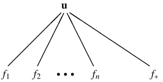
conditionally independent given u, see Figure 1, such that
p(f∗,f) ' q(f∗,f) = Z
q(f∗|u)q(f|u)p(u)du. (8)
The name inducing variable is motivated by the fact that f and f∗ can only communicate though u, and u therefore induces the dependencies between training and test cases. As we shall detail in the following sections, the different computationally efficient algorithms proposed in the literature correspond to different additional assumptions about the two approximate inducing conditionals
q(f|u), q(f∗|u)of the integral in (8). It will be useful for future reference to specify here the exact expressions for the two conditionals
training conditional: p(f|u) =
N
(Kf,uKu−,u1u,Kf,f−Qf,f), (9a)test conditional: p(f∗|u) =
N
(K∗,uKu−,u1u,K∗,∗−Q∗,∗), (9b) where we have introduced the shorthand notation6Qa,b,Ka,uKu−,1uKu,b. We can readily identify the expressions in (9) as special (noise free) cases of the standard predictive equation (6) with u playing the role of (noise free) observations. Note that the (positive semi-definite) covariance matrices in (9) have the form K−Q with the following interpretation: the prior covariance K minus a (non-negativedefinite) matrix Q quantifying how much information u provides about the variables in question (f or f∗). We emphasize that all the sparse methods discussed in the paper correspond simply to different approximations to the conditionals in (9), and throughout we use the exact likelihood and inducing prior
p(y|f) =
N
(f,σ2noiseI), and p(u) =
N
(0,Ku,u). (10)3. The Subset of Data (SoD) Approximation
Before we get started with the more sophisticated approximations, we mention as a baseline method the simplest possible sparse approximation (which doesn’t fall inside our general scheme): use only a subset of the data (SoD). The computational complexity is reduced to
O
(m3), where m<n.We would not generally expect SoD to be a competitive method, since it would seem impossible (even with fairly redundant data and a good choice of the subset) to get a realistic picture of the
A A A A A A Q Q Q Q Q Q Q Q Q u
f1 f2 r r r f
n f∗
r r A A A A A A Q Q Q Q Q Q Q Q Q u
f1 f2 r r r f
n f∗
r r
Figure 1: Graphical model of the relation between the inducing variables u, the training latent func-tions values f= [f1, . . . ,fn]>and the test function value f∗. The thick horizontal line
rep-resents a set of fully connected nodes. The observations y1, . . . ,yn,y∗(not shown) would dangle individually from the corresponding latent values, by way of the exact (factored) likelihood (5). Left graph: the fully connected graph corresponds to the case where no approximation is made to the full joint Gaussian process distribution between these variables. The inducing variables u are superfluous in this case, since all latent func-tion values can communicate with all others. Right graph: assumpfunc-tion of condifunc-tional
independence between training and test function values given u. This gives rise to the
separation between training and test conditionals from (8). Notice that having cut the communication path between training and test latent function values, information from f can only be transmitted to f∗via the inducing variables u.
uncertainties, when only a part of the training data is even considered. We include it here mostly as a baseline against which to compare better sparse approximations.
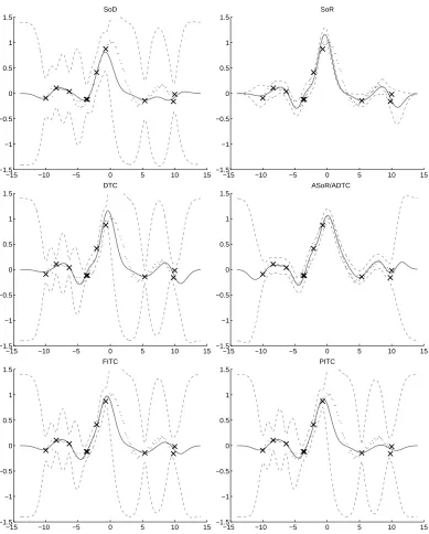
In Figure 5 top, left we see how the SoD method produces wide predictive distributions, when training on a randomly selected subset of 10 cases. A fair comparison to other methods would take into account that the computational complexity is independent of n as opposed to other more advanced methods. These extra computational resources could be spent in a number of ways, e.g. larger m, or an active (rather than random) selection of the m points. In this paper we will concentrate on understanding the theoretical foundations of the various approximations rather than investigating the necessary heuristics needed to turn the approximation schemes into actually prac-tical algorithms.
4. The Subset of Regressors (SoR) Approximation
The Subset of Regressors (SoR) algorithm was given by Silverman (1985), and mentioned again by Wahba et al. (1999). It was then adapted by Smola and Bartlett (2001) to propose a sparse greedy approximation to Gaussian process regression. SoR models are finite linear-in-the-parameters mod-els with a particular prior on the weights. For any input x∗, the corresponding function value f∗is given by:
which is Gaussian with zero mean and covariance
u = Ku,uwu ⇒ hu u>i = Ku,uhwuw>uiKu,u = Ku,u. (12)
Using the effective prior on u and the fact that wu=Ku−,u1u we can redefine the SoR model in an equivalent, more intuitive way:
f∗ = K∗,uKu−,u1u, with u ∼
N
(0,Ku,u). (13) We are now ready to integrate the SoR model in our unifying framework. Given that there is adeterministic relation between any f∗and u, the approximate conditional distributions in the integral in eq. (8) are given by:
qSoR(f|u) =
N
(Kf,uKu−,1uu,0), and qSoR(f∗|u) =N
(K∗,uKu−,1uu,0), (14) with zero conditional covariance, compare to (9). The effective prior implied by the SoR approxi-mation is easily obtained from (8), givingqSoR(f,f∗) =
N
0,hQf,f Qf,∗Q∗,f Q∗,∗
i
, (15)
where we recall Qa,b,Ka,uKu−,1uKu,b. A more descriptive name for this method, would be the Deterministic Inducing Conditional (DIC) approximation. We see that this approximate prior is degenerate. There are only m degrees of freedom in the model, which implies that only m linearly independent functions can be drawn from the prior. The m+1-th one is a linear combination of the previous. For example, in a very low noise regime, the posterior could be severely constrained by only m training cases.
The degeneracy of the prior causes unreasonable predictive distributions. Indeed, the approx-imate prior over functions is so restrictive, that given enough data only a very limited family of functions will be plausible under the posterior, leading to overconfident predictive variances. This is a general problem of finite linear models with small numbers of weights (for more details see Rasmussen and Qui˜nonero-Candela, 2005). Figure 5, top, right panel, illustrates the unreasonable predictive uncertainties of the SoR approximation on a toy dataset.7
The predictive distribution is obtained by using the SoR approximate prior (15) instead of the true prior in (4). For each algorithm we give two forms of the predictive distribution, one which is easy to interpret, and the other which is economical to compute with:
qSoR(f∗|y) =
N
Q∗,f(Qf,f+σ2noiseI)−1y,Q∗,∗−Q∗,f(Qf,f+σ2noiseI)−1Qf,∗
, (16a)
=
N
σ−2K∗,uΣKu,fy,K∗,uΣKu,∗, (16b)
where we have defined Σ= (σ−2K
u,fKf,u+Ku,u)−1. Equation (16a) is readily recognized as the regular prediction equation (6), except that the covariance K has everywhere been replaced by Q, which was already suggested by (15). This corresponds to replacing the covariance function k with
kSoR(xi,xj) =k(xi,u)Ku−,1uk(u,xj). The new covariance function has rank (at most) m. Thus we have the following
Remark 4 The SoR approximation is equivalent to exact inference in the degenerate Gaussian
process with covariance function kSoR(xi,xj) =k(xi,u)Ku−,1uk(u,xj).
The equivalent (16b) is computationally cheaper, and with (11) in mind,Σis the covariance of the posterior on the weights wu. Note that as opposed to the subset of data method, all training cases are taken into account. The computational complexity is
O
(nm2)initially, andO
(m)andO
(m2)per test case for the predictive mean and variance respectively.5. The Deterministic Training Conditional (DTC) Approximation
Taking up ideas already contained in the work of Csat´o and Opper (2002), Seeger et al. (2003) recently proposed another sparse approximation to Gaussian process regression, which does not suffer from the nonsensical predictive uncertainties of the SoR approximation, but that interestingly leads to exactly the same predictive mean. Seeger et al. (2003), who called the method Projected Latent Variables (PLV), presented the method as relying on a likelihood approximation, based on the projection f=Kf,uKu−,u1u:
p(y|f) ' q(y|u) =
N
(Kf,uKu−,1uu,σ2noiseI). (17) The method has also been called the Projected Process Approximation (PPA) by Rasmussen and Williams (2006, Chapter 8). One way of obtaining an equivalent model is to retain the usual likeli-hood, but to impose a deterministic training conditional and the exact test conditional from eq. (9b)qDTC(f|u) =
N
(Kf,uKu−,u1u,0), and qDTC(f∗|u) = p(f∗|u). (18) This reformulation has the advantage of allowing us to stick to our view of exact inference (with exact likelihood) with approximate priors. Indeed, under this model the conditional distribution of f given u is identical to that of the SoR, given in the left of (14). A systematic name for this approximation is the Deterministic Training Conditional (DTC).The fundamental difference with SoR is that DTC uses the exact test conditional (9b) instead of the deterministic relation between f∗and u of SoR. The joint prior implied by DTC is given by:
qDTC(f,f∗) =
N
0,hQf,f Qf,∗Q∗,f K∗,∗
i
, (19)
which is surprisingly similar to the effective prior implied by the SoR approximation (15). The fundamental difference is that under the DTC approximation f∗ has a prior variance of its own, given by K∗,∗. This prior variance reverses the behaviour of the predictive uncertainties, and turns
them into sensible ones, see Figure 5 for an illustration. The predictive distribution is now given by:
qDTC(f∗|y) =
N
(Q∗,f(Qf,f+σ2noiseI)−1y,K∗,∗−Q∗,f(Qf,f+σ2noiseI)−1Qf,∗ (20a)=
N
σ−2K∗,uΣKu,fy,K∗,∗−Q∗,∗+K∗,uΣK∗>,u
, (20b)
where again we have definedΣ= (σ−2K
u,fKf,u+Ku,u)−1 as in (16). The predictive mean for the DTC is identical to that of the SoR approximation (16), but the predictive variance replaces the Q∗,∗
from SoR with K∗,∗ (which is larger, since K∗,∗−Q∗,∗is positive definite). This added term is the
predictive variance of the posterior of f∗conditioned on u. It grows to the prior variance K∗,∗as x∗
A A A A A A
Q Q Q Q Q Q Q Q Q u
f1 f2 r r r f
n f∗
Figure 2: Graphical model for the FITC approximation. Compared to those in Figure 1, all edges between latent function values have been removed: the latent function values are con-ditionally fully independent given the inducing variables u. Although strictly speaking the SoR and DTC approximations could also be represented by this graph, note that both further assume a deterministic relation between f and u.
Remark 5 The only difference between the predictive distribution of DTC and SoR is the variance.
The predictive variance of DTC is never smaller than that of SoR.
Note, that since the covariances for training cases and test cases are computed differently, see (19), it follows that
Remark 6 The DTC approximation does not correspond exactly to a Gaussian process,
as the covariance between latent values depends on whether they are considered training or test cases, violating consistency, see Definition 1. The computational complexity has the same order as for SoR.
6. The Fully Independent Training Conditional (FITC) Approximation
Recently Snelson and Ghahramani (2006) proposed another likelihood approximation to speed up Gaussian process regression, which they called Sparse Gaussian Processes using Pseudo-inputs (SGPP). While the DTC is based on the likelihood approximation given by (17), the SGPP proposes a more sophisticated likelihood approximation with a richer covariance
p(y|f) ' q(y|u) =
N
(Kf,uKu−,1uu,diag[Kf,f−Qf,f] +σ2noiseI), (21) where diag[A] is a diagonal matrix whose elements match the diagonal of A. As we did in (18) for the DTC, we provide an alternative equivalent formulation called Fully Independent Training Conditional (FITC) based on the inducing conditionals:qFITC(f|u) = n
∏
i=1
p(fi|u) =
N
Kf,uKu−,1uu,diag[Kf,f−Qf,f]
, and qFITC(f∗|u) = p(f∗|u). (22)
section, we initially consider only a single test case, f∗. The corresponding graphical model is given in Figure 2. The effective prior implied by the FITC is given by
qFITC(f,f∗) =
N
0,hQf,f−diag[Qf,f−Kf,f] Qf,∗Q∗,f K∗,∗
i
. (23)
Note, that the sole difference between the DTC and FITC is that in the top left corner of the implied prior covariance, FITC replaces the approximate covariances of DTC by the exact ones on the diagonal. The predictive distribution is
qFITC(f∗|y) =
N
Q∗,f(Qf,f+Λ)−1y,K∗,∗−Q∗,f(Qf,f+Λ)−1Qf,∗
(24a)
=
N
K∗,uΣKu,fΛ−1y,K∗,∗−Q∗,∗+K∗,uΣKu,∗, (24b)where we have definedΣ= (Ku,u+Ku,fΛ−1Kf,u)−1andΛ=diag[Kf,f−Qf,f+σ2noiseI]. The compu-tational complexity is identical to that of SoR and DTC.
So far we have only considered a single test case. There are two options for joint predictions, either 1) use the exact full test conditional from (9b), or 2) extend the additional factorizing as-sumption to the test conditional. Although Snelson and Ghahramani (2006) don’t explicitly discuss joint predictions, it would seem that they probably intend the second option. Whereas the addi-tional independence assumption for the test cases is not really necessary for computaaddi-tional reasons, it does affect the nature of the approximation. Under option 1) the training and test covariance are computed differently, and thus this does not correspond to our strict definition of a GP model, but
Remark 7 Iff the assumption of full independence is extended to the test conditional, the FITC
ap-proximation is equivalent to exact inference in a non-degenerate Gaussian process with covariance function kFIC(xi,xj) =kSoR(xi,xj) +δi,j[k(xi,xj)−kSoR(xi,xj)],
whereδi,j is Kronecker’s delta. A logical name for the method where the conditionals (training and test) are always forced to be fully independent would be the Fully Independent Conditional (FIC) approximation. The effective prior implied by FIC is:
qFIC(f,f∗) =
N
0,hQf,f−diag[Qf,f−Kf,f] Qf,∗Q∗,f Q∗,∗−diag[Q∗,∗−K∗,∗]
i
. (25)
7. The Partially Independent Training Conditional (PITC) Approximation
In the previous section we saw how to improve the DTC approximation by approximating the train-ing conditional with an independent distribution, i.e. one with a diagonal covariance matrix. In this section we will further improve the approximation (while remaining computationally attractive) by extending the training conditional to have a block diagonal covariance:
qPITC(f|u) =
N
Kf,uKu−,u1u,blockdiag[Kf,f−Qf,f]
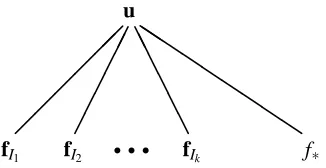
, and qPITC(f∗|u) = p(f∗|u). (26) where blockdiag[A]is a block diagonal matrix (where the blocking structure is not explicitly stated). We represent graphically the PITC approximation in Figure 3. Developing this analogously to the FITC approximation from the previous section, we get the joint prior
qPITC(f,f∗) =
N
0,hQf,f−blockdiag[Qf,f−Kf,f] Qf,∗Q∗,f K∗,∗
i
A A A A A A
Q Q Q Q Q Q Q Q Q u
fI1 fI2 r r r fIk f∗
Figure 3: Graphical representation of the PITC approximation. The set of latent function values fIi
indexed by the the set of indices Ii is fully connected. The PITC differs from FITC (see graph in Fig. 2) in that conditional independence is now between the k groups of training latent function values. This corresponds to the block diagonal approximation to the true training conditional given in (26).
and the predictive distribution is identical to (24), except for the alternative definition of Λ= blockdiag[Kf,f−Qf,f+σ2noiseI]. An identical expression was obtained by Schwaighofer and Tresp (2003, Sect. 3), developing from the original Bayesian committee machine (BCM) by Tresp (2000). The relationship to the FITC was pointed out by Lehel Csat´o. The BCM was originally proposed as a transductive learner (i.e. where the test inputs have to be known before training), and the inducing inputs Xuwere chosen to be the test inputs. We discuss transduction in detail in the next section.
It is important to realize that the BCM proposes two orthogonal ideas: first, the block diagonal structure of the partially independent training conditional, and second setting the inducing inputs to be the test inputs. These two ideas can be used independently and in Section 8 we propose using the first without the second.
The computational complexity of the PITC approximation depends on the blocking structure imposed in (26). A reasonable choice, also recommended by Tresp (2000) may be to choose
k=n/m blocks, each of size m×m. The computational complexity remains
O
(nm2). Since in the PITC model the covariance is computed differently for training and test casesRemark 8 The PITC approximation does not correspond exactly to a Gaussian process.
This is because computing covariances requires knowing whether points are from the training- or test-set, (27). One can obtain a Gaussian process from the PITC by extending the partial conditional independence assumption to the test conditional, as we did in Remark 7 for the FITC.
8. Transduction and Augmentation
The idea of transduction is that one should restrict the goal of learning to prediction on a pre-specified set of test cases, rather than trying to learn an entire function (induction) and then evaluate it at the test inputs. There may be no universally agreed upon definition of transduction. In this paper we use
Definition 9 Transduction occurs only if the predictive distribution depends on other test inputs.
A A A A A A
u
fI1 fI2
r r r f
Ik f∗
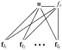
Figure 4: Two views on Augmentation. One view is to see that the test latent function value f∗ is now part of the inducing variables u and therefore has access to the training latent function values. An equivalent view is to consider that we have dropped the assumption of conditional independence between f∗ and the training latent function values. Even if
f∗ has now direct access to each of the training fi, these still need to go through u to talk to each other if they fall in conditionally independent blocks. We have in this figure decided to recycle the graph for PITC from Figure 3 to show that all approximations we have presented can be augmented, irrespective of what the approximation for the training conditional is.
There are several different possible motivations for transduction: 1) transduction is somehow easier than induction (Vapnik, 1995), 2) the test inputs may reveal important information, which should be used during training. This motivation drives models in semi-supervised learning (studied mostly in the context of classification) and 3) for approximate algorithms one may be able to limit the discrepancies of the approximation at the test points.
For exact GP models it seems that the first reason doesn’t really apply. If you make predictions at the test points that are consistent with a GP, then it is trivial inside the GP framework to extend these to any other input points, and in effect we have done induction.
The second reason seems more interesting. However, in a standard GP setting, it is a conse-quence of the consistency property, see Remark 2, that predictions at one test input are independent of the location of any other test inputs. Therefore transduction can not be married with exact GPs:
Remark 10 Transduction can not occur in exact Gaussian process models.
Whereas this holds for the usual setting of GPs, it could be different in non-standard situations where e.g. the covariance function depends on the empirical input densities.
Transduction can occur in the sparse approximation to GPs, by making the choice of inducing variables depend on the test inputs. The BCM from the previous section, where Xu=X∗ (where X∗are the test inputs) is an example of this. Since the inducing variables are connected to all other nodes (see Figure 3) we would expect the approximation to be good at u=f∗, which is what we care about for predictions, relating to reason 3) above. While this reasoning is sound, it is not necessarily a sufficient consideration for getting a good model. The model has to be able to simultaneously explain the training targets as well and if the choice of u makes this difficult, the posterior at the points of interest may be distorted. Thus, the choice of u should be governed by the ability to model the conditional of the latents given the inputs, and not solely by the density of the (test) inputs.
involved in the predictive distributions (e.g. matrix inversion) before seeing the test cases, enabling fast computation of test predictions.
It is interesting that whereas other methods spend much effort trying to optimize the inducing variables, the BCM simply uses the test set. The quality of the BCM approximation depends then on the particular location of the test inputs, upon which one usually does not have any control. We now see that there may be a better method, eliminating the drawback of transduction, namely use the PITC approximation, but choose the u’s carefully (see Section 9), don’t just use the test set.
8.1 Augmentation
An idea closely related to transduction, but not covered by our definition, is augmentation, which in contrast to transduction is done individually for each test case. Since in the previous sections, we haven’t assumed anything about u, we can simply augment the set of inducing variables by f∗ (i.e. have one additional inducing variable equal to the current test latent), and see what happens in the predictive distributions for the different methods. Let’s first investigate the consequences for the test conditional from (9b). Note, the interpretation of the covariance matrix K∗,∗−Q∗,∗
was “the prior covariance minus the information which u provides about f∗”. It is clear that the augmented u (with f∗) provides all possible information about f∗, and consequently Q∗,∗=K∗,∗.
An equivalent view on augmentation is that the assumption of conditional independence between
f∗ and f is dropped. This is seen trivially by adding edges between f∗ and the fi in the graphical model, Figure 4.
Augmentation was originally proposed by Rasmussen (2002), and applied in detail to the SoR with RBF covariance by Qui˜nonero-Candela (2004). Because the SoR is a finite linear model, and the basis functions are local (Gaussian bumps), the predictive distributions can be very misleading. For example, when making predictions far away from the center of any basis function, all basis functions have insignificant magnitudes, and the prediction (averaged over the posterior) will be close to zero, with very small error-bars; this is the opposite of the desired behaviour, where we would expect the error-bars to grow as we move away from the training cases. Here augmentation makes a particularly big difference turning the nonsensical predictive distribution into a reasonable one, by ensuring that there is always a basis function centered on the test case. Compare the non-augmented to the non-augmented SoR in Figure 5. An analogous Gaussian process based finite linear model that has recently been healed by augmentation is the relevance vector machine (Rasmussen and Qui˜nonero-Candela, 2005).
Although augmentation was initially proposed for a narrow set of circumstances, it is easily applied to any of the approximations discussed. Of course, augmentation doesn’t make any sense for an exact, non-degenerate Gaussian process model (a GP with a covariance function that has a feature-space which is infinite dimensional, i.e. with basis functions everywhere).
Remark 11 A full non-degenerate Gaussian process cannot be augmented,
since the corresponding f∗would already be connected to all other variables in the graphical model. But augmentation does make sense for sparse approximations to GPs.
however, it seems clear that one would chose the additional inducing variable to be f∗, to minimize the effects of the approximations.
Let us compute the effective prior for the augmented SoR. Given that f∗ is in the inducing set, the test conditional is not an approximation and we can rewrite the integral leading to the effective prior:
qASoR(f∗,f) = Z
qSoR(f|f∗,u)p(f∗,u)du. (28) It is interesting to notice that this is also the effective prior that would result from augmenting the DTC approximation, since qSoR(f|f∗,u) =qDTC(f|f∗,u).
Remark 12 Augmented SoR (ASoR) is equivalent to augmented DTC (ADTC).
Augmented DTC only differs from DTC in the additional presence of f∗among the inducing vari-ables in the training conditional. We can only expect augmented DTC to be a more accurate approx-imation than DTC, since adding an additional inducing variable can only help capture information from y. Therefore
Remark 13 DTC is a less accurate (but cheaper) approximation than augmented SoR.
We saw previously in Section 5 that the DTC approximation does not suffer from the nonsensi-cal predictive variances of the SoR. The equivalence between the augmented SoR and augmented DTC is another way of seeing how augmentation reverses the misbehaviour of SoR. The predictive distribution of the augmented SoR is obtained by adding f∗to u in (20).
Prediction with an augmented sparse model comes at a higher computational cost, since now f∗ directly interacts with all of f and not just with u. For each new test case, updating the augmentedΣ in the predictive equation (for example (20b) for DTC) implies computing the vector matrix product
K∗,fKf,uwith complexity
O
(nm). This is clearly higher than theO
(m)for the mean, andO
(m2)for the predictive distribution of all the non-augmented methods we have discussed.Augmentation seems to be only really necessary for methods that make a severe approxima-tion to the test condiapproxima-tional, like the SoR. For methods that make little or no approximaapproxima-tion to the test conditional, it is difficult to predict the degree to which augmentation would help. However, one can see by giving f∗access to all of the training latent function values in f, one would expect augmentation to give less under-confident predictive distributions near the training data. Figure 5 clearly shows that augmented DTC (equivalent to augmented SoR) has a superior predictive dis-tribution (both mean and variance) than standard DTC. Note however that in the figure we have purposely chosen a too short lengthscale to enhance visualization. Quantitatively, this superiority was experimentally assessed by Qui˜nonero-Candela (2004, Table 3.1). Augmentation hasn’t been compared to the more advanced approximations FITC and PITC, and the figure would change in the more realistic scenario where the inducing inputs and hyperparameters are learnt (Snelson and Ghahramani, 2006).
Transductive methods like the BCM can be seen as joint augmentation, and one could potentially use it for any of the methods presented. It seems that the good performance of the BCM could essentially stem from augmentation, the presence of the other test inputs in the inducing set being probably of little benefit. Joint augmentation might bring some computational advantage, but won’t change the scaling: note that augmenting m times at a cost of
O
(nm) apiece implies the same−15 −10 −5 0 5 10 15 −1.5
−1 −0.5 0 0.5 1 1.5
SoD
−15 −10 −5 0 5 10 15 −1.5
−1 −0.5 0 0.5 1 1.5
SoR
−15 −10 −5 0 5 10 15 −1.5
−1 −0.5 0 0.5 1 1.5
DTC
−15 −10 −5 0 5 10 15 −1.5
−1 −0.5 0 0.5 1 1.5
ASoR/ADTC
−15 −10 −5 0 5 10 15 −1.5
−1 −0.5 0 0.5 1 1.5
FITC
−15 −10 −5 0 5 10 15 −1.5
−1 −0.5 0 0.5 1 1.5
PITC
9. On the Choice of the Inducing Variables
We have until now assumed that the inducing inputs Xuwere given. Traditionally, sparse models have very often been built upon a carefully chosen subset of the training inputs. This concept is probably best exemplified in the popular support vector machine (Cortes and Vapnik, 1995). In sparse Gaussian processes it has also been suggested to select the inducing inputs Xufrom among the training inputs. Since this involves a prohibitive combinatorial optimization, greedy optimiza-tion approaches have been suggested using various selecoptimiza-tion criteria like online learning (Csat´o and Opper, 2002), greedy posterior maximization (Smola and Bartlett, 2001), maximum information gain (Seeger et al., 2003), matching pursuit (Keerthi and Chu, 2006), and probably more. As dis-cussed in the previous section, selecting the inducing inputs from among the test inputs has also been considered in transductive settings. Recently, Snelson and Ghahramani (2006) have proposed to relax the constraint that the inducing variables must be a subset of training/test cases, turning the discrete selection problem into one of continuous optimization. One may hope that finding a good solution is easier in the continuous than the discrete case, although finding the global optimum is intractable in both cases. And perhaps the less restrictive choice can lead to better performance in very sparse models.
Which optimality criterion should be used to set the inducing inputs? Departing from a fully Bayesian treatment which would involve defining priors on Xu, one could maximize the marginal likelihood (also called the evidence) with respect to Xu, an approach also followed by Snelson and Ghahramani (2006). Each of the approximate methods proposed involves a different effective prior, and hence its own particular effective marginal likelihood conditioned on the inducing inputs
q(y|Xu) = ZZ
p(y|f)q(f|u)p(u|Xu)du df= Z
p(y|f)q(f|Xu)df, (29)
which of course is independent of the test conditional. We have in the above equation explicitly conditioned on the inducing inputs Xu. Using Gaussian identities, the effective marginal likelihood is very easily obtained by adding a ridgeσ2noiseI (from the likelihood) to the covariance of effective
prior on f. Using the appropriate definitions ofΛ, the log marginal likelihood becomes
log q(y|Xu) = −12log|Qf,f+Λ| −12y>(Qf,f+Λ)−1y−n2log(2π), (30) where ΛSoR=ΛDTC =σ2noiseI, ΛFITC =diag[Kf,f−Qf,f] +σ2noiseI, and ΛPITC =blockdiag[Kf,f−
Qf,f] +σ2noiseI. The computational cost of the marginal likelihood is
O
(nm2)for all methods, that of its gradient with respect to one element of XuisO
(nm). This of course implies that the complexity of computing the gradient wrt. to the whole of XuisO
(dnm2), where d is the dimension of the input space.It has been proposed to maximize the effective posterior instead of the effective marginal likeli-hood (Smola and Bartlett, 2001). However this is potentially dangerous and can lead to overfitting. Maximizing the whole evidence instead is sound and comes at an identical computational cost (for a deeper analysis see Qui˜nonero-Candela, 2004, Sect. 3.3.5 and Fig. 3.2).
10. Other Methods
In this section we briefly mention two approximations which don’t fit in our unifying scheme, since one doesn’t correspond to a proper probabilistic model, and the other one uses a particular construction for the covariance function, rather than allowing any general covariance function.
10.1 The Nystr¨om Approximation
The Nystr¨om Approximation for speeding up GP regression was originally proposed by Williams and Seeger (2001), and then questioned by Williams et al. (2002). Like SoR and DTC, the Nystr¨om Approximation for GP regression approximates the prior covariance of f by Qf,f. However, unlike these methods, the Nystr¨om Approximation is not based on a generative probabilistic model. The prior covariance between f∗and f is taken to be exact, which is inconsistent with the prior covariance on f:
q(f,f∗) =
N
0,hQf,f Kf,∗K∗,f K∗,∗
i
. (31)
As a result we cannot derive this method from our unifying framework, nor represent it with a graphical model. Worse, the resulting prior covariance matrix is not even guaranteed to be positive definite, allowing the predictive variances to be negative. Notice that replacing Kf,∗by Qf,∗ in (31)
is enough to make the prior covariance positive definite, and one obtains the DTC approximation.
Remark 14 The Nystr¨om Approximation does not correspond to a well-formed probabilistic model.
Ignoring any quibbles about positive definiteness, the predictive distribution of the Nystr¨om Ap-proximation is given by:
p(f∗|y) =
N
Kf>,∗[Qf,f+σ2noiseI]−1y,K∗,∗−Kf>,∗[Qf,f+σ2noiseI]−1Kf,∗, (32)but the predictive variance is not guaranteed to be positive. The computational cost is
O
(nm2). 10.2 The Relevance Vector MachineThe relevance vector machine, introduced by Tipping (2001), is a finite linear model with an in-dependent Gaussian prior imposed on the weights. For any input x∗, the corresponding function output is given by:
f∗ = φ∗w, with p(w|A) =
N
(0,A), (33)whereφ∗= [φ1(x), . . . ,φm(x)]is the (row) vector of responses of the m basis functions, and A= diag(α1, . . . ,αm)is the diagonal matrix of joint prior precisions (inverse variances) of the weights. Theαi are learnt by maximizing the RVM evidence (obtained by also assuming Gaussian additive iid. noise, see (1)), and for the typical case of rich enough sets of basis functions many of the precisions go to infinity effectively pruning out the corresponding weights (for a very interesting analysis see Wipf et al., 2004). The RVM is thus a sparse method and the surviving basis functions are called relevance vectors.
Note that since the RVM is a finite linear model with Gaussian priors on the weights, it can be seen as a Gaussian process:
Remark 15 The RVM is equivalent to a degenerate Gaussian process with covariance function
kRVM(xi,xj) =φiA−1φ>j =∑mk=1α− 1
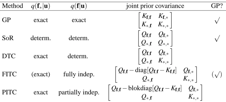
Method q(f∗|u) q(f|u) joint prior covariance GP?
GP exact exact
Kf,f Kf,∗ K∗,f K∗,∗
√
SoR determ. determ.
Qf,f Qf,∗ Q∗,f Q∗,∗
√
DTC exact determ.
Qf,f Qf,∗ Q∗,f K∗,∗
FITC (exact) fully indep.
Qf,f−diag[Qf,f−Kf,f] Qf,∗ Q∗,f K∗,∗
(√)
PITC exact partially indep.
Qf,f−blokdiag[Qf,f−Kf,f] Qf,∗
Q∗,f K∗,∗
Table 1: Summary of the way approximations are built. All these methods are detailed in the previ-ous sections. The initial cost and that of the mean and variance per test case are respectively
n2, n and n2for the exact GP, and nm2, m and m2for all other methods. The “GP?” column indicates whether the approximation is equivalent to a GP. For FITC see Remark 7.
as was also pointed out by Tipping (2001, eq. (59)). Whereas all sparse approximations we have presented until now are totally independent of the choice of covariance function, for the RVM this choice is restricted to covariance functions that can be expressed as finite expansions in terms of some basis functions. Being degenerate GPs in exactly the same way as the SoR (presented in Section 4), the RVM does also suffer from unreasonable predictive variances. Rasmussen and Qui˜nonero-Candela (2005) show that the predictive distributions of RVMs can also be healed by augmentation, see Section 8. Once theαihave been learnt, denoting by m the number of surviving relevance vectors, the complexity of computing the predictive distribution of the RVM is
O
(m)for mean andO
(m2)for the variance.RVMs are often used with radial basis functions centered on the training inputs. One potentially interesting extension to the RVM would be to learn the locations of the centers of the basis functions, in the same way as proposed by Snelson and Ghahramani (2006) for the FITC approximation, see Section 6. This is a curious reminiscence of learning the centers in RBF Networks.
11. Conclusions
We have provided a unifying framework for sparse approximations to Gaussian processes for regres-sion. Our approach consists of two steps, first 1) we recast the approximation in terms of approx-imations to the prior, and second 2) we introduce inducing variables u and the idea of conditional independence given u. We recover all existing sparse methods by making further simplifications of the covariances of the training and test conditionals, see Table 1 for a summary.
and Ghahramani (2006) contains two ideas, 1) a likelihood approximation and 2) the idea of varying the inducing inputs continuously; these two ideas could easily be used independently, and incorpo-rated in other methods. Similarly, the BCM by Tresp (2000) contains two independent ideas 1) a block diagonal assumption, and 2) the (transductive) idea of choosing the test inputs as the induc-ing variables. Finally we note that although all three ideas of 1) transductively settinduc-ing u=f∗, 2) augmentation and 3) continuous optimization of Xuhave been proposed in very specific settings, in fact they are completely general ideas, which can be applied to any of the approximation schemes considered.
We have ranked the approximation according to how close they are to the corresponding full GP. However, the performance in practical situations may not always follow this theoretical ranking since the approximations might exhibit properties (not present in the full GP) which may be par-ticularly suitable for specific datasets. This may make the interpretation of empirical comparisons challenging. A further complication arises when adding the necessary heuristics for turning the theoretical constructs into practical algorithms. We have not described full algorithms in this paper, but are currently working on a detailed empirical study (in preparation, see also Rasmussen and Williams, 2006, chapter 8).
We note that the order of the computational complexity is identical for all the methods consid-ered,
O
(nm2). This highlights that there is no computational excuse for using gross approximations, such as assuming deterministic relationships, in particular one should probably think twice before using SoR or even DTC. Although augmentation has attractive predictive properties, it is com-putationally expensive. It remains unclear whether augmentation could be beneficial on a fixed computational budget.We have only considered the simpler case of regression in this paper, but sparseness is also com-monly sought in classification settings. It should not be difficult to cast probabilistic approximation methods such as Expectation Propagation (EP) or the Laplace method (for a comparison, see Kuss and Rasmussen, 2005) into our unifying framework.
Our analysis suggests that a new interesting approximation would come from combining the best possible approximation (PITC) with the most powerful selection method for the inducing inputs. This would correspond to a non-transductive version of the BCM. We would evade the necessity of knowing the test set before doing the bulk of the computation, and we could hope to supersede the superior performance reported by Snelson and Ghahramani (2006) for very sparse approximations.
Acknowledgments
Appendix A. Gaussian and Matrix Identities
In this appendix we provide identities used to manipulate matrices and Gaussian distributions throughout the paper. Let x and y be jointly Gaussian
x y
∼
N
µx
µy
,
A C
C> B
, (34)
then the marginal and the conditional are given by
x ∼
N
(µx,A), and x|y ∼N
µx+C B−1(y−µy),A−C B−1C>
(35)
Also, the product of a Gaussian in x with a Gaussian in a linear projection P x is again a Gaussian, although unnormalized
N
(x|a,A)N
(P x|b,B) = zcN
(x|c,C), (36)where
C = A−1+P>B−1P−1, c = C A−1a+P>B−1b.
The normalizing constant zcis gaussian in the means a and b of the two Gaussians:
zc = (2π)−
m
2|B+P A P>|− 1
2 exp
−1
2(b−P a)> B+P A P>
−1
(b−P a). (37)
The matrix inversion lemma, also known as the Woodbury, Sherman & Morrison formula states that:
(Z+UWV>)−1 = Z−1−Z−1U(W−1+V>Z−1U)−1V>Z−1, (38) assuming the relevant inverses all exist. Here Z is n×n, W is m×m and U and V are both of size n×m; consequently if Z−1is known, and a low rank (ie. m<n) perturbation are made to Z as in
left hand side of eq. (38), considerable speedup can be achieved.
References
Corinna Cortes and Vladimir Vapnik. Support-vector network. Machine Learning, 20(3):273–297, 1995.
Lehel Csat´o and Manfred Opper. Sparse online Gaussian processes. Neural Computation, 14(3): 641–669, 2002.
Sathiya Keerthi and Wei Chu. A Matching Pursuit approach to sparse Gaussian process regression. In Y. Weiss, B. Sch¨olkopf, and J. Platt, editors, Advances in Neural Information Processing
Systems 18, Cambridge, Massachussetts, 2006. The MIT Press.
Malte Kuss and Carl Edward Rasmussen. Assessing approximate inference for binary Gaussian process classification. Journal of Machine Learning Research, pages 1679–1704, 2005.
Joaquin Qui˜nonero-Candela. Learning with Uncertainty – Gaussian Processes and Relevance
Vec-tor Machines. PhD thesis, Technical University of Denmark, Lyngby, Denmark, 2004.
Carl Edward Rasmussen and Joaquin Qui˜nonero-Candela. Healing the relevance vector machine by augmentation. In International Conference on Machine Learning, 2005.
Carl Edward Rasmussen and Christopher K. I. Williams. Gaussian Processes for Machine Learning. The MIT press, 2006.
Anton Schwaighofer and Volker Tresp. Transductive and inductive methods for approximate Gaus-sian process regression. In Suzanna Becker, Sebastian Thrun, and Klaus Obermayer, editors,
Advances in Neural Information Processing Systems 15, pages 953–960, Cambridge,
Massachus-setts, 2003. The MIT Press.
Matthias Seeger, Christopher K. I. Williams, and Neil Lawrence. Fast forward selection to speed up sparse Gaussian process regression. In Christopher M. Bishop and Brendan J. Frey, editors, Ninth
International Workshop on Artificial Intelligence and Statistics. Society for Artificial Intelligence
and Statistics, 2003.
Bernhard W. Silverman. Some aspects of the spline smoothing approach to non-parametric regres-sion curve fitting. J. Roy. Stat. Soc. B, 47(1):1–52, 1985. (with discusregres-sion).
Alexander J. Smola and Peter L. Bartlett. Sparse greedy Gaussian process regression. In Todd K. Leen, Thomas G. Dietterich, and Volker Tresp, editors, Advances in Neural Information
Process-ing Systems 13, pages 619–625, Cambridge, Massachussetts, 2001. The MIT Press.
Edward Snelson and Zoubin Ghahramani. Sparse Gaussian processes using pseudo-inputs. In Y. Weiss, B. Sch¨olkopf, and J. Platt, editors, Advances in Neural Information Processing Systems
18, Cambridge, Massachussetts, 2006. The MIT Press.
Michael E. Tipping. Sparse Bayesian learning and the Relevance Vector Machine. Journal of
Machine Learning Research, 1:211–244, 2001.
Volker Tresp. A Bayesian committee machine. Neural Computation, 12(11):2719–2741, 2000.
Vladimir N. Vapnik. The Nature of Statistical Learning Theory. Springer Verlag, 1995.
Grace Wahba, Xiwu Lin, Fangyu Gao, Dong Xiang, Ronald Klein, and Barbara Klein. The bias-variance tradeoff and the randomized GACV. In Michael S. Kerns, Sara A. Solla, and David A. Cohn, editors, Advances in Neural Information Processing Systems 11, pages 620–626, Cam-bridge, Massachussetts, 1999. The MIT Press.
Christopher K. I. Williams and Carl Edward Rasmussen. Gaussian processes for regression. In David S. Touretzky, Michael C. Mozer, and Michael E. Hasselmo, editors, Advances in Neural
Information Processing Systems 8, pages 514–520, Cambridge, Massachussetts, 1996. The MIT
Press.
Christopher K. I. Williams and Mathias Seeger. Using the Nystr¨om method to speed up kernel machines. In Todd K. Leen, Thomas G. Dietterich, and Volker Tresp, editors, Advances in Neural
Information Processing Systems 13, pages 682–688, Cambridge, Massachussetts, 2001. The MIT
Press.
David Wipf, Jason Palmer, and Bhaskar Rao. Perspectives on sparse Bayesian learning. In Sebas-tian Thrun, Lawrence Saul, and Bernhard Sch¨olkopf, editors, Advances in Neural Information
![Figure 1: Graphical model of the relation between the inducing variables u, the training latent func-tions values f = [f1,..., fn]⊤ and the test function value f∗](https://thumb-us.123doks.com/thumbv2/123dok_us/9840978.1970452/5.612.102.512.89.173/figure-graphical-relation-inducing-variables-training-latent-function.webp)