Boosting as a Regularized Path to a Maximum Margin Classifier

Boosting as a Regularized Path

to a Maximum Margin Classifier

Saharon Rosset [email protected]

Data Analytics Research Group IBM T.J. Watson Research Center Yorktown Heights, NY 10598, USA

Ji Zhu [email protected]

Department of Statistics University of Michigan Ann Arbor, MI 48109, USA

Trevor Hastie [email protected]

Department of Statistics Stanford University Stanford, CA 94305,USA

Editor: Robert Schapire

Abstract

In this paper we study boosting methods from a new perspective. We build on recent work by Efron et al. to show that boosting approximately (and in some cases exactly) minimizes its loss criterion with an l1constraint on the coefficient vector. This helps understand the success of boosting with early stopping as regularized fitting of the loss criterion. For the two most commonly used crite-ria (exponential and binomial log-likelihood), we further show that as the constraint is relaxed—or equivalently as the boosting iterations proceed—the solution converges (in the separable case) to an “l1-optimal” separating hyper-plane. We prove that this l1-optimal separating hyper-plane has the property of maximizing the minimal l1-margin of the training data, as defined in the boosting liter-ature. An interesting fundamental similarity between boosting and kernel support vector machines emerges, as both can be described as methods for regularized optimization in high-dimensional predictor space, using a computational trick to make the calculation practical, and converging to margin-maximizing solutions. While this statement describes SVMs exactly, it applies to boosting only approximately.

Keywords: boosting, regularized optimization, support vector machines, margin maximization

1. Introduction and Outline

Boosting is a method for iteratively building an additive model

FT(x) = T

∑

αthjt(x), (1)

where hjt ∈

H

learners”; and hjt is the basis function selected as the “best candidate” to modify the function at

function h∈

H

FT(x) = J

∑

hj(x)·β(jT), (2)

where J=|H|andβ(_jT)=∑jt=jαt. The “β” representation allows us to interpret the coefficient

vectorβ(T)as a vector in

R

interpretation will play a key role in our exposition. Some examples of common dictionaries are:

• The training variables themselves, in which case hj(x) =xj. This leads to our “additive”

model FT being just a linear model in the original data. The number of dictionary functions

will be J=d, the dimension of x.

• Polynomial dictionary of degree p, in which case the number of dictionary functions will be

J=

p+d d

.

• Decision trees with up to k terminal nodes, if we limit the split points to data points (or

mid-way between data points as CART does). The number of possible trees is bounded from above (trivially) by J≤(np)k_·2k2

. Note that regression trees do not fit into our framework,

since they will give J=∞.

The boosting idea was first introduced by Freund and Schapire (1995), with their AdaBoost algorithm. AdaBoost and other boosting algorithms have attracted a lot of attention due to their great success in data modeling tasks, and the “mechanism” which makes them work has been presented and analyzed from several perspectives. Friedman et al. (2000) develop a statistical perspective, which ultimately leads to viewing AdaBoost as a gradient-based incremental search for a good additive model (more specifically, it is a “coordinate descent” algorithm), using the exponential loss

function C(y,F) =exp(−yF), where y∈ {−1,1}. The gradient boosting (Friedman, 2001) and

anyboost (Mason et al., 1999) generic algorithms have used this approach to generalize the boosting idea to wider families of problems and loss functions. In particular, Friedman et al. (2000) have

pointed out that the binomial log-likelihood loss C(y,F) =log(1+exp(−yF)) is a more natural

loss for classification, and is more robust to outliers and misspecified data.

A different analysis of boosting, originating in the machine learning community, concentrates on

the effect of boosting on the margins yiF(xi). For example, Schapire et al. (1998) use margin-based

arguments to prove convergence of boosting to perfect classification performance on the training data under general conditions, and to derive bounds on the generalization error (on future, unseen data).

In this paper we combine the two approaches, to conclude that gradient-based boosting can be described, in the separable case, as an approximate margin maximizing process. The view we de-velop of boosting as an approximate path of optimal solutions to regularized problems also justifies early stopping in boosting as specifying a value for “regularization parameter”.

We consider the problem of minimizing non-negative convex loss functions (in particular the

exponential and binomial log-likelihood loss functions) over the training data, with an l1bound on

the model coefficients:

ˆ

β(c) =arg min

kβk1≤c

∑

Where h(xi) = [h1(xi),h2(xi), . . . ,hJ(xi)]0 _{and J=|}

_H

Hastie et al. (2001, Chapter 10) have observed that “slow” gradient-based boosting (i.e., we set

αt =ε,∀t in (1), with εsmall) tends to follow the penalized path βˆ(c)as a function of c, under

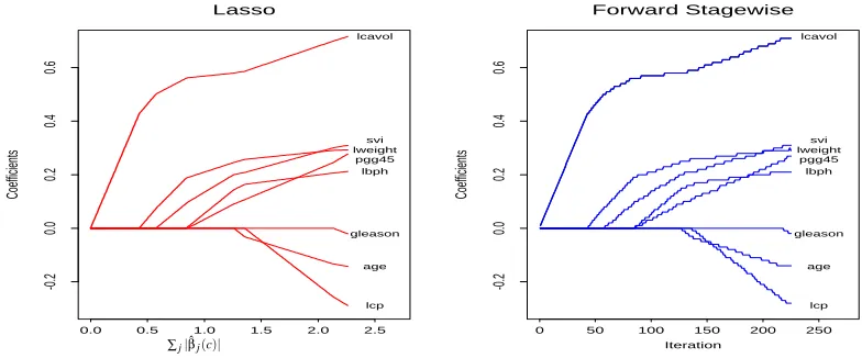
some mild conditions on this path. In other words, using the notation of (2), (3), this implies that kβ(c/ε)_−βˆ_{(c)k vanishes with ε, for all (or a wide range of) values of c. Figure 1 illustrates this}

equivalence betweenε-boosting and the optimal solution of (3) on a real-life data set, using squared

error loss as the loss function. In this paper we demonstrate this equivalence further and formally

Coefficients

0.0 0.5 1.0 1.5 2.0 2.5

-0.2

0.0

0.2

0.4

0.6

Lasso

lcavol

lweight

age lbph svi

lcp gleason

pgg45

Iteration

Coefficients

0 50 100 150 200 250

-0.2

0.0

0.2

0.4

0.6

Forward Stagewise

lcavol

lweight

age lbph svi

lcp gleason

pgg45

PSfrag replacements

∑j|βˆj(c)|

Figure 1: Exact coefficient paths(left) for l1-constrained squared error regression and “boosting”

coefficient paths (right) on the data from a prostate cancer study

state it as a conjecture. Some progress towards proving this conjecture has been made by Efron et al. (2004), who prove a weaker “local” result for the case where C is squared error loss, under some mild conditions on the optimal path. We generalize their result to general convex loss functions.

Combining the empirical and theoretical evidence, we conclude that boosting can be viewed as

an approximate incremental method for following the l1-regularized path.

We then prove that in the separable case, for both the exponential and logistic log-likelihood

loss functions,βˆ(c)/cconverges as c→∞to an “optimal” separating hyper-planeβˆdescribed by

ˆ

β=arg max

kβk1=1 min

i yiβ

0_{h(xi). (4)}

In other words,βˆ maximizes the minimal margin among all vectors with l1-norm equal to 1.2 This

result generalizes easily to other lp-norm constraints. For example, if p=2, thenβˆ describes the

optimal separating hyper-plane in the Euclidean sense, i.e., the same one that a non-regularized support vector machine would find.

Combining our two main results, we get the following characterization of boosting:

1. Our notation assumes that the minimum in (3) is unique, which requires some mild assumptions. To avoid notational complications we use this slightly abusive notation throughout this paper. In Appendix B we give explicit conditions for uniqueness of this minimum.

ε-Boosting can be described as a gradient-descent search, approximately following the

path of l1-constrained optimal solutions to its loss criterion, and converging, in the

separable case, to a “margin maximizer” in the l1sense.

Note that boosting with a large dictionary

H

H

will be separable (except for pathologies), hence separability is a very mild assumption here.

As in the case of support vector machines in high dimensional feature spaces, the non-regularized “optimal” separating hyper-plane is usually of theoretical interest only, since it typically represents an over-fitted model. Thus, we would want to choose a good regularized model. Our results indicate that Boosting gives a natural method for doing that, by “stopping early” in the boosting process. Fur-thermore, they point out the fundamental similarity between Boosting and SVMs: both approaches allow us to fit regularized models in high-dimensional predictor space, using a computational trick.

They differ in the regularization approach they take—exact l2regularization for SVMs, approximate

l1regularization for Boosting—-and in the computational trick that facilitates fitting—the “kernel”

trick for SVMs, coordinate descent for Boosting.

1.1 Related Work

Schapire et al. (1998) have identified the normalized margins as distance from an l1-normed

sep-arating hyper-plane. Their results relate the boosting iterations’ success to the minimal margin of the combined model. R¨atsch et al. (2001b) take this further using an asymptotic analysis of Ad-aBoost. They prove that the “normalized” minimal margin, miniyi∑tαtht(xi)/∑t|αt|, is

asymptoti-cally equal for both classes. In other words, they prove that the asymptotic separating hyper-plane is equally far away from the closest points on either side. This is a property of the margin maximizing separating hyper-plane as we define it. Both papers also illustrate the margin maximizing effects of AdaBoost through experimentation. However, they both stop short of proving the convergence to optimal (margin maximizing) solutions.

Motivated by our result, R¨atsch and Warmuth (2002) have recently asserted the margin-maximizing

properties ofε-AdaBoost, using a different approach than the one used in this paper. Their results

relate only to the asymptotic convergence of infinitesimal AdaBoost, compared to our analysis of the “regularized path” traced along the way and of a variety of boosting loss functions, which also leads to a convergence result on binomial log-likelihood loss.

The convergence of boosting to an “optimal” solution from a loss function perspective has been analyzed in several papers. R¨atsch et al. (2001a) and Collins et al. (2000) give results and bounds on the convergence of training-set loss,∑_iC(yi,∑tαtht(xi)), to its minimum. However, in the separable

case convergence of the loss to 0 is inherently different from convergence of the linear separator to the optimal separator. Any solution which separates the two classes perfectly can drive the expo-nential (or log-likelihood) loss to 0, simply by scaling coefficients up linearly.

Two recent papers have made the connection between boosting and l1regularization in a slightly

different context than this paper. Zhang (2003) suggests a “shrinkage” version of boosting which

converges to l1regularized solutions, while Zhang and Yu (2003) illustrate the quantitative

2. Boosting as Gradient Descent

Generic gradient-based boosting algorithms (Friedman, 2001; Mason et al., 1999) attempt to find a good linear combination of the members of some dictionary of basis functions to optimize a given loss function over a sample. This is done by searching, at each iteration, for the basis function which gives the “steepest descent” in the loss, and changing its coefficient accordingly. In other words,

this is a “coordinate descent” algorithm inRJ, where we assign one dimension (or coordinate) for

the coefficient of each dictionary function.

Assume we have data {xi,yi}ni=1 with xi∈Rd, a loss (or cost) function C(y,F), and a set of

dictionary functions {hj(x)}:Rd →R. Then all of these algorithms follow the same essential

steps:

Algorithm 1 Generic gradient-based boosting algorithm

1. Setβ(0)=0.

2. For t =1 : T ,

(a) Let Fi=β(t−1) 0

h(xi),i=1, . . . ,n (the current fit). (b) Set wi=∂C(yi,Fi)

∂Fi ,i=1, . . . ,n.

(c) Identify jt=arg maxj|∑iwihj(xi)|. (d) Setβ(_jt)

t =β

(t−1)

jt −αtsign(∑iwihjt(xi))andβ (t)

k =β

(t−1)

k ,k6= jt.

Hereβ(t)is the “current” coefficient vector andαt>0 is the current step size. Notice that∑iwihjt(xi) =

∂∑iC(yi,Fi)

∂βjt .

As we mentioned, Algorithm 1 can be interpreted simply as a coordinate descent algorithm in

“weak learner” space. Implementation details include the dictionary

H

function C(y,F), the method of searching for the optimal jt and the way in whichαt is determined.3

For example, the original AdaBoost algorithm uses this scheme with the exponential loss C(y,F) =

exp(−yF), and an implicit line search to find the bestαt once a “direction” jt has been chosen (see

Hastie et al., 2001; Mason et al., 1999). The dictionary used by AdaBoost in this formulation would

be a set of candidate classifiers, i.e., hj(xi)∈ {−1,+1}—usually decision trees are used in practice.

2.1 Practical Implementation of Boosting

The dictionaries used for boosting are typically very large—practically infinite—and therefore the generic boosting algorithm we have presented cannot be implemented verbatim. In particular, it is not practical to exhaustively search for the maximizer in step 2(c). Instead, an approximate, usually

greedy search is conducted to find a “good” candidate weak learner hjt which makes the first order

decline in the loss large (even if not maximal among all possible models).

In the common case that the dictionary of weak learners is comprised of decision trees with up to k nodes, the way AdaBoost and other boosting algorithms solve stage 2(c) is by building a

3. The sign ofαtwill always be−sign(∑iwihjt(xi)), since we want the loss to be reduced. In most cases, the dictionary

decision tree to a re-weighted version of the data, with the weights|wi|. Thus they first replace step 2(c) with minimization of

∑

|wi|1{yi6=hjt(xi)},

which is easily shown to be equivalent to the original step 2(c). They then use a greedy decision-tree building algorithm such as CART or C5 to build a k-node decision decision-tree which minimizes this quantity, i.e., achieves low “weighted misclassification error” on the weighted data. Since the tree is built greedily—one split at a time—it will not be the global minimizer of weighted misclassification error among all k-node decision trees. However, it will be a good fit for the re-weighted data, and can be considered an approximation to the optimal tree.

This use of approximate optimization techniques is critical, since much of the strength of the boosting approach comes from its ability to build additive models in very high-dimensional predic-tor spaces. In such spaces, standard exact optimization techniques are impractical: any approach which requires calculation and inversion of Hessian matrices is completely out of the question, and even approaches which require only first derivatives, such as coordinate descent, can only be implemented approximately.

2.2 Gradient-Based Boosting as a Generic Modeling Tool

As Friedman (2001); Mason et al. (1999) mention, this view of boosting as gradient descent allows us to devise boosting algorithms for any function estimation problem—all we need is an appro-priate loss and an approappro-priate dictionary of “weak learners”. For example, Friedman et al. (2000) suggested using the binomial log-likelihood loss instead of the exponential loss of AdaBoost for binary classification, resulting in the LogitBoost algorithm. However, there is no need to limit boosting algorithms to classification—Friedman (2001) applied this methodology to regression es-timation, using squared error loss and regression trees, and Rosset and Segal (2003) applied it to density estimation, using the log-likelihood criterion and Bayesian networks as weak learners. Their experiments and those of others illustrate that the practical usefulness of this approach—coordinate descent in high dimensional predictor space—carries beyond classification, and even beyond super-vised learning.

The view we present in this paper, of coordinate-descent boosting as approximate l1-regularized

fitting, offers some insight into why this approach would be good in general: it allows us to fit regu-larized models directly in high dimensional predictor space. In this it bears a conceptual similarity

to support vector machines, which exactly fit an l2regularized model in high dimensional (RKH)

predictor space.

2.3 Loss Functions

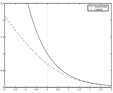
The two most commonly used loss functions for boosting classification models are the exponential and the (minus) binomial log-likelihood:

Exponential : Ce(y,F) =exp(−yF);

Loglikelihood : Cl(y,F) =log(1+exp(−yF)).

−2 −1.5 −1 −0.5 0 0.5 1 1.5 2 2.5 3 0

0.5 1 1.5 2 2.5

Exponential Logistic

Figure 2: The two classification loss functions

given by

ˆ

F(x) =c·log

P(y=1|x) P(y=−1|x)

,

where ce=1/2 for exponential loss and cl=1 for binomial loss.

More importantly for our purpose, we have the following simple proposition, which illustrates the strong similarity between the two loss functions for positive margins (i.e., correct classifica-tions):

Proposition 1

yF≥0⇒0.5Ce(y,F)≤Cl(y,F)≤Ce(y,F). (5)

In other words, the two losses become similar if the margins are positive, and both behave like exponentials.

Proof Consider the functions f1(z) =z and f2(z) =log(1+z)for z∈[0,1]. Then f1(0) =f2(0) =0,

and

∂f1(z)

∂z ≡1

1

2 ≤

∂f2(z) ∂z =

1

1+z ≤1.

Thus we can conclude 0.5 f1(z)≤ f2(z)≤ f1(z). Now set z=exp(−y f) and we get the desired

result.

For negative margins the behaviors of Ce and Cl are very different, as Friedman et al. (2000)

have noted. In particular, Clis more robust against outliers and misspecified data.

2.4 Line-Search Boosting vs.ε-Boosting

As mentioned above, AdaBoost determinesαt using a line search. In our notation for Algorithm 1

this would be

αt =arg min_α

∑

The alternative approach, suggested by Friedman (2001); Hastie et al. (2001), is to “shrink” allαt

to a single small valueε. This may slow down learning considerably (depending on how small ε

is), but is attractive theoretically: the first-order theory underlying gradient boosting implies that the weak learner chosen is the best increment only “locally”. It can also be argued that this

ap-proach is “stronger” than line search, as we can keep selecting the same hjt repeatedly if it remains

optimal and so ε-boosting dominates line-search boosting in terms of training error. In practice,

this approach of “slowing the learning rate” usually performs better than line-search in terms of

prediction error as well (see Friedman, 2001). For our purposes, we will mostly assume ε is

in-finitesimally small, so the theoretical boosting algorithm which results is the “limit” of a series of

boosting algorithms with shrinkingε.

In regression terminology, the line-search version is equivalent to forward stage-wise modeling, infamous in the statistics literature for being too greedy and highly unstable (see Friedman, 2001). This is intuitively obvious, since by increasing the coefficient until it saturates we are destroying “signal” which may help us select other good predictors.

3. lpMargins, Support Vector Machines and Boosting

We now introduce the concept of margins as a geometric interpretation of a binary classification model. In the context of boosting, this view offers a different understanding of AdaBoost from the gradient descent view presented above. In the following sections we connect the two views.

3.1 The Euclidean Margin and the Support Vector Machine

Consider a classification model in high dimensional predictor space: F(x) =∑_jhj(x)βj. We say

that the model separates the training data{xi,yi}n

i=1 if sign(F(xi)) =yi, ∀i. From a geometrical

perspective this means that the hyper-plane defined by F(x) =0 is a separating hyper-plane for this

data, and we define its (Euclidean) margin as

m2(β) =min i

yiF(xi)

kβk2

. (6)

The margin-maximizing separating hyper-plane for this data would be defined by β which

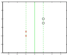
max-imizes m2(β). Figure 3 shows a simple example of separable data in two dimensions, with its

margin-maximizing separating plane. The Euclidean margin-maximizing separating hyper-plane is the (non regularized) support vector machine solution. Its margin maximizing properties play a central role in deriving generalization error bounds for these models, and form the basis for a rich literature.

3.2 The l1Margin and Its Relation to Boosting

Instead of considering the Euclidean margin as in (6) we can define an “lpmargin” concept as

mp(β) =min

i

yiF(xi)

kβkp

. (7)

Of particular interest to us is the case p=1. Figure 4 shows the l1margin maximizing separating

−3 −2 −1 0 1 2 3 −3

−2 −1 0 1 2 3

Figure 3: A simple data example, with two observations from class “O” and two observations from class “X”. The full line is the Euclidean margin-maximizing separating hyper-plane.

−3 −2 −1 0 1 2 3

−3 −2 −1 0 1 2 3

Figure 4: l1 margin maximizing separating hyper-plane for the same data set as Figure 3. The

difference between the diagonal Euclidean optimal separator and the vertical l1 optimal

the two solutions: the l2-optimal separator is diagonal, while the l1-optimal one is vertical. To

understand why this is so we can relate the two margin definitions to each other as

yF(x)

kβk1

=yF(x)

kβk2

·kβk2 kβk1

. (8)

From this representation we can observe that the l1 margin will tend to be big if the ratio k_kβ_βk_k2₁ is

big. This ratio will generally be big ifβis sparse. To see this, consider fixing the l1 norm of the

vector and then comparing the l2norm of two candidates: one with many small components and the

other—a sparse one—with a few large components and many zero components. It is easy to see that

the second vector will have bigger l2norm, and hence (if the l2 margin for both vectors is equal) a

bigger l1margin.

A different perspective on the difference between the optimal solutions is given by a theorem

due to Mangasarian (1999), which states that the lp margin maximizing separating hyper plane

maximizes the lq distance from the closest points to the separating hyper-plane, with 1_p+1_q =1.

Thus the Euclidean optimal separator (p=2) also maximizes Euclidean distance between the points

and the hyper-plane, while the l1optimal separator maximizes l∞distance. This interesting result

gives another intuition why l1 optimal separating hyper-planes tend to be coordinate-oriented (i.e.,

have sparse representations): since l_∞ projection considers only the largest coordinate distance,

some coordinate distances may be 0 at no cost of decreased l_∞distance.

Schapire et al. (1998) have pointed out the relation between AdaBoost and the l1margin. They

prove that, in the case of separable data, the boosting iterations increase the “boosting” margin of the model, defined as

min

i

yiF(xi) kαk1

. (9)

In other words, this is the l1margin of the model, except that it uses theαincremental representation

rather than theβ“geometric” representation for the model. The two representations give the same

l1norm if there is sign consistency, or “monotonicity” in the coefficient paths traced by the model,

i.e., if at every iteration t of the boosting algorithm

βjt 6=0⇒sign(αt) =sign(βjt). (10)

As we will see later, this monotonicity condition will play an important role in the equivalence

between boosting and l1regularization.

The l1-margin maximization view of AdaBoost presented by Schapire et al. (1998)—and a

whole plethora of papers that followed—is important for the analysis of boosting algorithms for two distinct reasons:

• It gives an intuitive, geometric interpretation of the model that AdaBoost is looking for—a

model which separates the data well in this l1-margin sense. Note that the view of boosting as

gradient descent in a loss criterion doesn’t really give the same kind of intuition: if the data is separable, then any model which separates the training data will drive the exponential or binomial loss to 0 when scaled up:

m1(β)>0 =⇒

∑

i

• The l1-margin behavior of a classification model on its training data facilitates generation

of generalization (or prediction) error bounds, similar to those that exist for support vector machines (Schapire et al., 1998). The important quantity in this context is not the margin but the “normalized” margin, which considers the “conjugate norm” of the predictor vectors:

yiβ0h(xi)

kβk1kh(xi)k∞

.

When the dictionary we are using is comprised of classifiers thenkh(xi)k_∞≡1 always and

thus the l1 margin is exactly the relevant quantity. The error bounds described by Schapire

et al. (1998) allow using the whole l1margin distribution, not just the minimal margin.

How-ever, boosting’s tendency to separate well in the l1 sense is a central motivation behind their

results.

From a statistical perspective, however, we should be suspicious of margin-maximization as a method for building good prediction models in high dimensional predictor space. Margin maxi-mization in high dimensional space is likely to lead to over-fitting and bad prediction performance. This has been observed in practice by many authors, in particular Breiman (1999). Our results in the next two sections suggest an explanation based on model complexity: margin maximization is the limit of parametric regularized optimization models, as the regularization vanishes, and the reg-ularized models along the path may well be superior to the margin maximizing “limiting” model, in terms of prediction performance. In Section 7 we return to discuss these issues in more detail.

4. Boosting as Approximate Incremental l1Constrained Fitting

In this section we introduce an interpretation of the generic coordinate-descent boosting algorithm

as tracking a path of approximate solutions to l1-constrained (or equivalently, regularized) versions

of its loss criterion. This view serves our understanding of what boosting does, in particular the connection between early stopping in boosting and regularization. We will also use this view to get a result about the asymptotic margin-maximization of regularized classification models, and by analogy of classification boosting. We build on ideas first presented by Hastie et al. (2001, Chapter 10) and Efron et al. (2004).

Given a convex non-negative loss criterion C(·,·), consider the 1-dimensional path of optimal

solutions to l1constrained optimization problems over the training data:

ˆ

β(c) =arg min

kβk1≤c

∑

C(yi,h(xi)0β). (11)

As c varies, we get that ˆβ(c) traces a 1-dimensional “optimal curve” through RJ. If an optimal

solution for the non-constrained problem exists and has finite l1 norm c0, then obviously ˆβ(c) =

ˆ

β(c0) =βˆ , ∀c>c0. in the case of separable 2-class data, using either Ceor Cl, there is no

finite-norm optimal solution. Rather, the constrained solution will always havekβˆ(c)k1=c.

A different way of building a solution which has l1 norm c, is to run ourε-boosting algorithm

for c/εiterations. This will give anα(c/ε)vector which has l1norm exactly c. For the norm of the

geometric representation β(c/ε) to also be equal to c, we need the monotonicity condition (10) to

hold as well. This condition will play a key role in our exposition.

Lasso

0 1000 2000 3000

-500

0

500

1 2

39 4 7 105 8 6 1

2 3 4 5 6 7 8 9 10 • • •• • • •• • • Stagwise

0 1000 2000 3000

-500

0

500

1 2

39 4 7 105 86 1

2 3 4 5 6 7 8 9 10 • • •• • • •• • •

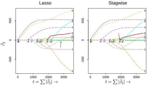
Figure 5: Another example of the equivalence between the Lasso optimal solution path (left) and

ε-boosting with squared error loss. Note that the equivalence breaks down when the path

of variable 7 becomes non-monotone

this similarity for squared error loss fitting with l1(lasso) penalty. Figure 5 shows another example

in the same mold, taken from Efron et al. (2004). The data is a diabetes study and the “dictionary”

used is just the original 10 variables. The panel on the left shows the path of optimal l1-constrained

solutions ˆβ(c)and the panel on the right shows theε-boosting path with the 10-dimensional

dictio-nary (the total number of boosting iterations is about 6000). The 1-dimensional path throughR10

is described by 10 coordinate curves, corresponding to each one of the variables. The interesting phenomenon we observe is that the two coefficient traces are not completely identical. Rather, they agree up to the point where variable 7 coefficient path becomes non monotone, i.e., it violates (10) (this point is where variable 8 comes into the model, see the arrow on the right panel). This example

illustrates that the monotonicity condition—and its implication thatkαk1=kβk1—is critical for the

equivalence betweenε-boosting and l1-constrained optimization.

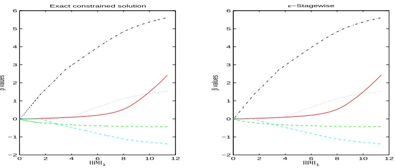
The two examples we have seen so far have used squared error loss, and we should ask ourselves whether this equivalence stretches beyond this loss. Figure 6 shows a similar result, but this time for

the binomial log-likelihood loss, Cl. We used the “spam” data set, taken from the UCI repository

(Blake and Merz, 1998). We chose only 5 predictors of the 57 to make the plots more interpretable and the computations more accommodating. We see that there is a perfect equivalence between the

exact constrained solution (i.e., regularized logistic regression) andε-boosting in this case, since the

paths are fully monotone.

To justify why this observed equivalence is not surprising, let us consider the following “l1

-locally optimal monotone direction” problem of finding the best monotoneεincrement to a given

modelβ0:

min C(β) (12)

s.t. kβk1− kβ0k1≤ε,

0 2 4 6 8 10 12 −2

−1 0 1 2 3 4 5 6

Exact constrained solution

||β||1

β

values

0 2 4 6 8 10 12 −2

−1 0 1 2 3 4 5 6

ε−Stagewise

||β||1

β

values

Figure 6: Exact coefficient paths (left) for l1-constrained logistic regression and boosting coefficient

paths (right) with binomial log-likelihood loss on five variables from the “spam” data set.

The boosting path was generated usingε=0.003 and 7000 iterations.

Here we use C(β)as shorthand for∑_iC(yi,h(xi)0β). A first order Taylor expansion gives us

C(β) =C(β0) +∇C(β0)0(β−β0) +O(ε2).

And given the l1constraint on the increase inkβk1, it is easy to see that a first-order optimal solution

(and therefore an optimal solution asε→0) will make a “coordinate descent” step, i.e.

βj6=β0,j ⇒ |∇C(β0)j|=max

k |∇C(β0)k|,

assuming the signs match, i.e., sign(β0 j) =−sign(∇C(β0)j).

So we get that if the optimal solution to (12) without the monotonicity constraint happens to be monotone, then it is equivalent to a coordinate descent step. And so it is reasonable to expect that if

the optimal l1regularized path is monotone (as it indeed is in Figures 1,6), then an “infinitesimal”

ε-boosting algorithm would follow the same path of solutions. Furthermore, even if the optimal

path is not monotone, we can still use the formulation (12) to argue thatε-boosting would tend to

follow an approximate l1-regularized path. The main difference between theε-boosting path and

the true optimal path is that it will tend to “delay” becoming non-monotone, as we observe for variable 7 in Figure 5. To understand this specific phenomenon would require analysis of the true optimal path, which falls outside the scope of our discussion—Efron et al. (2004) cover the subject for squared error loss, and their discussion applies to any continuously differentiable convex loss, using second-order approximations.

We can employ this understanding of the relationship between boosting and l1 regularization

to construct lpboosting algorithms by changing the coordinate-selection criterion in the coordinate

descent algorithm. We will get back to this point in Section 7, where we design an “l2boosting”

algorithm.

The experimental evidence and heuristic discussion we have presented lead us to the following

Conjecture 2 Consider applying theε-boosting algorithm to any convex loss function, generating a path of solutions β(ε)(t). Then if the optimal coefficient paths are monotone ∀c<c0, i.e., if

∀j, |βˆ(c)j|is non-decreasing in the range c<c0, then

lim

ε→0β

(ε)_{(c0/ε) =βˆ(c0).}

Efron et al. (2004, Theorem 2) prove a weaker “local” result for the case of squared error loss only. We generalize their result to any convex loss. However this result still does not prove the “global” convergence which the conjecture claims, and the empirical evidence implies. For the sake of brevity and readability, we defer this proof, together with concise mathematical definition of the different types of convergence, to appendix A.

In the context of “real-life” boosting, where the number of basis functions is usually very large,

and making εsmall enough for the theory to apply would require running the algorithm forever,

these results should not be considered directly applicable. Instead, they should be taken as an

intu-itive indication that boosting—especially theεversion—is, indeed, approximating optimal solutions

to the constrained problems it encounters along the way.

5. lp-Constrained Classification Loss Functions

Having established the relation between boosting and l1 regularization, we are going to turn our

attention to the regularized optimization problem. By analogy, our results will apply to boosting

as well. We concentrate on Ce and Cl, the two classification losses defined above, and the solution

paths of their lpconstrained versions:

ˆ

β(p)_{(c) =arg min}

kβkp≤c

∑

C(yi,β0h(xi)). (13)

where C is either Ce or Cl. As we discussed below Equation (11), if the training data is separable in

span(

H

p=c for all values of c. Consequently

kβˆ

(p)_(c)

c kp=1.

We may ask what are the convergence points of this sequence as c→∞. The following theorem

shows that these convergence points describe “lp-margin maximizing” separating hyper-planes.

Theorem 3 Assume the data is separable, i.e.,∃βs.t.∀i,yiβ0h(xi)>0.

Then for both Ceand Cl, every convergence point of βˆ(_cc) corresponds to an lp-margin-maximizing separating hyper-plane.

If the lp-margin-maximizing separating hyper-plane is unique, then it is the unique convergence points, i.e.

ˆ

β(p)_{= lim}

c→∞

ˆ

β(p)_(c)

c =arg maxkβkp=1

min

i yiβ 0_h(x

i). (14)

Proof This proof applies to both Ce and Cl, given the property in (5). Consider two separating

candidatesβ1andβ2such thatkβ1kp=kβ2kp=1. Assume thatβ1separates better, i.e. m1:=min

i yiβ 0

1h(xi)>m2:=min i yiβ

0

2h(xi)>0.

Lemma 4 There exists some D=D(m1,m2)such that∀d>D, dβ1incurs smaller loss than dβ2, in other words:

∑

C(yi,dβ01h(xi))<

∑

C(yi,dβ02h(xi)).

Given this lemma, we can now prove that any convergence point of βˆ(p_c)(c) must be an lp-margin

maximizing separator. Assumeβ∗ is a convergence point of βˆ(p_c)(c). Denote its minimal margin on

the data by m∗. If the data is separable, clearly m∗>0 (since otherwise the loss of dβ∗ does not

even converge to 0 as d→∞).

Now, assume some ˜βwithkβ˜kp=1 has bigger minimal margin ˜m>m∗. By continuity of the

minimal margin inβ, there exists some open neighborhood ofβ∗

N_β∗ ={β:kβ−β∗k₂<δ}

and anε>0, such that

min

i yiβ 0_h(x

i)<m˜−ε, ∀β∈Nβ∗.

Now by the lemma we get that there exists some D=D(m˜,m˜ −ε)such that d ˜βincurs smaller

loss than dβfor any d>D,β∈N_β∗. Thereforeβ∗cannot be a convergence point of

ˆ

β(p)_(c)

c .

We conclude that any convergence point of the sequence βˆ(p_c)(c) must be an lp-margin

maximiz-ing separator. If the margin maximizmaximiz-ing separator is unique then it is the only possible convergence point, and therefore

ˆ

β(p)_{= lim}

c→∞

ˆ

β(p)_(c)

c =arg maxkβkp=1

min

i yiβ 0_h(xi).

Proof of Lemma Using (5) and the definition of Ce, we get for both loss functions:

∑

i

C(yi,dβ01h(xi))≤n exp(−d·m1).

Now, sinceβ1separates better, we can find our desired

D=D(m1,m2) =logn+log2 m1−m2

such that

∀d>D, n exp(−d·m1)<0.5 exp(−d·m2).

And using (5) and the definition of Ceagain we can write

0.5 exp(−d·m2)≤

∑

i

C(yi,dβ0₂h(xi)). Combining these three inequalities we get our desired result:

∀d>D,

∑

i

C(yi,dβ01h(xi))≤

∑

i

We thus conclude that if the lp-margin maximizing separating hyper-plane is unique, the

nor-malized constrained solution converges to it. In the case that the margin maximizing separating hyper-plane is not unique, we can in fact prove a stronger result, which indicates that the limit of the regularized solutions would then be determined by the second smallest margin, then by the third and so on. This result is mainly of technical interest and we prove it in Appendix B, Section 2.

5.1 Implications of Theorem 3

We now briefly discuss the implications of this theorem for boosting and logistic regression.

5.1.1 BOOSTINGIMPLICATIONS

Combined with our results from Section 4, Theorem 3 indicates that the normalized boosting path

β(t)

∑u≤tαu—with either Ce or Cl used as loss—“approximately” converges to a separating hyper-plane

ˆ

β, which attains

max

kβk1=1 min

i yiβ 0_h(x

i) = max

kβk1=1

kβk2min

i yidi, (15)

where diis the (signed) Euclidean distance from the training point i to the separating hyper-plane. In

other words, it maximizes Euclidean distance scaled by an l2norm. As we have mentioned already,

this implies that the asymptotic boosting solution will tend to be sparse in representation, due to the

fact that for fixed l1norm, the l2 norm of vectors that have many 0 entries will generally be larger.

In fact, under rather mild conditions, the asymptotic solution ˆβ=limc→∞βˆ(1)(c)/c, will have at most n (the number of observations) non-zero coefficients, if we use either Cl or Ce as the loss. See

Appendix B, Section 1 for proof.

5.1.2 LOGISTICREGRESSIONIMPLICATIONS

Recall, that the logistic regression (maximum likelihood) solution is undefined if the data is sepa-rable in the Euclidean space spanned by the predictors. Theorem 3 allows us to define a logistic regression solution for separable data, as follows:

1. Set a high constraint value cmax

2. Find ˆβ(p)(cmax), the solution to the logistic regression problem subject to the constraintkβkp≤

cmax. The problem is convex for any p≥1 and differentiable for any p>1, so interior point

methods can be used to solve this problem.

3. Now you have (approximately) the lp-margin maximizing solution for this data, described by

ˆ

β(p)_(c

max) cmax .

This is a solution to the original problem in the sense that it is, approximately, the convergence

Of course, with our result from Theorem 3 it would probably make more sense to simply find the

optimal separating hyper-plane directly—this is a linear programming problem for l1separation and

a quadratic programming problem for l2separation. We can then consider this optimal separator as

a logistic regression solution for the separable data.

6. Examples

We now apply boosting to several data sets and interpret the results in light of our regularization and margin-maximization view.

6.1 Spam Data Set

We now know if the data are separable and we let boosting run forever, we will approach the same

“optimal” separator for both Ceand Cl. However if we stop early—or if the data is not separable—

the behavior of the two loss functions may differ significantly, since Ce weighs negative margins

exponentially, while Cl is approximately linear in the margin for large negative margins (see

Fried-man et al., 2000). Consequently, we can expect Ceto concentrate more on the “hard” training data,

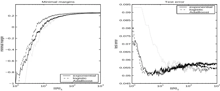
in particular in the non-separable case. Figure 7 illustrates the behavior of ε-boosting with both

100

101

102

103

−1 −0.8 −0.6 −0.4 −0.2 0 0.2

Minimal margins

||β||1

minimal margin

exponential logistic AdaBoost

100

101

102

103

0.045 0.05 0.055 0.06 0.065 0.07 0.075 0.08 0.085 0.09 0.095

Test error

||β||1

test error

exponential logistic AdaBoost

Figure 7: Behavior of boosting with the two loss functions on spam data set

loss functions, as well as that of AdaBoost, on the spam data set (57 predictors, binary response).

We used 10 node trees andε=0.1. The left plot shows the minimal margin as a function of the

l1 norm of the coefficient vector kβk1. Binomial loss creates a bigger minimal margin initially,

but the minimal margins for both loss functions are converging asymptotically. AdaBoost initially lags behind but catches up nicely and reaches the same minimal margin asymptotically. The right

plot shows the test error as the iterations proceed, illustrating that bothε-methods indeed seem to

over-fit eventually, even as their “separation” (minimal margin) is still improving. AdaBoost did not significantly over-fit in the 1000 iterations it was allowed to run, but it obviously would have if it were allowed to run on.

We should emphasize that the comparison between AdaBoost andε-boosting presented

consid-ers as a basis for comparison the l1norm, not the number of iterations. In terms of computational

mar-gin and good prediction performance much more quickly than the “slow boosting” approaches, as AdaBoost tends to take larger steps.

6.2 Simulated Data

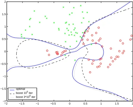
To make a more educated comparison and more compelling visualization, we have constructed an example of separation of 2-dimensional data using a 8-th degree polynomial dictionary (45 func-tions). The data consists of 50 observations of each class, drawn from a mixture of Gaussians, and

presented in Figure 8. Also presented, in the solid line, is the optimal l1 separator for this data in

this dictionary (easily calculated as a linear programming problem - note the difference from the l2

optimal decision boundary, presented in Section 7.1, Figure 11 ). The optimal l1separator has only

12 non-zero coefficients out of 45.

−2 −1.5 −1 −0.5 0 0.5 1 1.5 2

−2 −1.5 −1 −0.5 0 0.5 1 1.5 2

optimal boost 105 iter boost 3*106 iter

Figure 8: Artificial data set with l1-margin maximizing separator (solid), and boosting models

af-ter 105 iterations (dashed) and 106 iterations (dotted) using ε=0.001. We observe the

convergence of the boosting separator to the optimal separator

We ran an ε-boosting algorithm on this data set, using the logistic log-likelihood loss Cl, with

ε=0.001, and Figure 8 shows two of the models generated after 105and 3·106iterations. We see

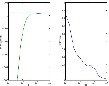
that the models seem to converge to the optimal separator. A different view of this convergence is given in Figure 9, where we see two measures of convergence: the minimal margin (left, maximum

value obtainable is the horizontal line) and the l1-norm distance between the normalized models

(right), given by

∑

ˆ

βj− β(t)

j

kβ(t)_k

1

,

where ˆβis the optimal separator with l1norm 1 andβ(t)is the boosting model after t iterations.

We can conclude that on this simple artificial example we get nice convergence of the

logistic-boosting model path to the l1-margin maximizing separating hyper-plane.

We can also use this example to illustrate the similarity between the boosted path and the path

101

102

103

104

−0.05 −0.04 −0.03 −0.02 −0.01 0 0.01

||β||1

Minimal margin

101

102

103

104

0 0.2 0.4 0.6 0.8 1 1.2 1.4 1.6 1.8 2

||β||1

l1

difference

Figure 9: Two measures of convergence of boosting model path to optimal l1 separator: minimal

margin (left) and l1distance between the normalized boosting coefficient vector and the

optimal model (right)

l

1 norm: 20 l1 norm: 350

l

1 norm: 2701 l1 norm: 5401

Figure 10: Comparison of decision boundary of boosting models (broken) and of optimal con-strained solutions with same norm (full)

Figure 10 shows the class decision boundaries for 4 models generated along the boosting path, compared to the optimal solutions to the constrained “logistic regression” problem with the same

bound on the l1 norm of the coefficient vector. We observe the clear similarities in the way the

solutions evolve and converge to the optimal l1separator. The fact that they differ (in some cases

(not shown), we observe that the monotonicity condition is consistently violated in the low norm ranges, and hence we can expect the paths to be similar in spirit but not identical.

7. Discussion

We can now summarize what we have learned about boosting from the previous sections:

• Boosting approximately follows the path of l1-regularized models for its loss criterion

• If the loss criterion is the exponential loss of AdaBoost or the binomial log-likelihood loss

of logistic regression, then the l1 regularized model converges to an l1-margin maximizing

separating hyper-plane, if the data are separable in the span of the weak learners

We may ask, which of these two points is the key to the success of boosting approaches. One empirical clue to answering this question, can be found in Breiman (1999), who programmed an algorithm to directly maximize the margins. His results were that his algorithm consistently got significantly higher minimal margins than AdaBoost on many data sets (and, in fact, a “higher” margin distribution beyond the minimal margin), but had slightly worse prediction performance. His conclusion was that margin maximization is not the key to AdaBoost’s success. From a statistical perspective we can embrace this conclusion, as reflecting the importance of regularization in high-dimensional predictor space. By our results from the previous sections, “margin maximization”

can be viewed as the limit of parametric regularized models, as the regularization vanishes.4 Thus

we would generally expect the margin maximizing solutions to perform worse than regularized models. In the case of boosting, regularization would correspond to “early stopping” of the boosting algorithm.

7.1 Boosting and SVMs as Regularized Optimization in High-dimensional Predictor Spaces

Our exposition has led us to view boosting as an approximate way to solve the regularized optimiza-tion problem

min

β

∑

0_{h(xi)) +λkβk}

1 (16)

which converges asλ→0 to ˆβ(1), if our loss is Ceor Cl. In general, the loss C can be any convex

differentiable loss and should be defined to match the problem domain.

Support vector machines can be described as solving the regularized optimization problem (see Friedman et al., 2000, Chapter 12)

min

β

∑

0_h(x

i))++λkβk22 (17)

which “converges” asλ→0 to the non-regularized support vector machine solution, i.e., the optimal

Euclidean separator, which we denoted by ˆβ(2).

An interesting connection exists between these two approaches, in that they allow us to solve the regularized optimization problem in high dimensional predictor space:

• We are able to solve the l1- regularized problem approximately in very high dimension via

boosting by applying the “approximate coordinate descent” trick of building a decision tree (or otherwise greedily selecting a weak learner) based on re-weighted versions of the data.

• Support vector machines facilitate a different trick for solving the regularized optimization

problem in high dimensional predictor space: the “kernel trick”. If our dictionary

H

a Reproducing Kernel Hilbert Space, then RKHS theory tells us we can find the regularized solutions by solving an n-dimensional problem, in the space spanned by the kernel represen-ters{K(xi,x)}. This fact is by no means limited to the hinge loss of (17), and applies to any

convex loss. We concentrate our discussion on SVM (and hence hinge loss) only since it is by far the most common and well-known application of this result.

So we can view both boosting and SVM as methods that allow us to fit regularized models in high dimensional predictor space using a computational “shortcut”. The complexity of the model built is controlled by regularization. These methods are distinctly different than traditional statistical approaches for building models in high dimension, which start by reducing the dimensionality of the problem so that standard tools (e.g., Newton’s method) can be applied to it, and also to make over-fitting less of a concern. While the merits of regularization without dimensionality reduction— like Ridge regression or the Lasso—are well documented in statistics, computational issues make it impractical for the size of problems typically solved via boosting or SVM, without computational tricks.

We believe that this difference may be a significant reason for the enduring success of boosting and SVM in data modeling, i.e.:

Working in high dimension and regularizing is statistically preferable to a two-step procedure of first reducing the dimension, then fitting a model in the reduced space.

It is also interesting to consider the differences between the two approaches, in the loss (flexible

vs. hinge loss), the penalty (l1 vs. l2), and the type of dictionary used (usually trees vs. RKHS).

These differences indicate that the two approaches will be useful for different situations. For

ex-ample, if the true model has a sparse representation in the chosen dictionary, then l1regularization

may be warranted; if the form of the true model facilitates description of the class probabilities via

a logistic-linear model, then the logistic loss Cl is the best loss to use, and so on.

The computational tricks for both SVM and boosting limit the kind of regularization that can be used for fitting in high dimensional space. However, the problems can still be formulated and solved for different regularization approaches, as long as the dimensionality is low enough:

• Support vector machines can be fitted with an l1penalty, by solving the 1-norm version of the

SVM problem, equivalent to replacing the l2penalty in (17) with an l1penalty. In fact, the

1-norm SVM is used quite widely, because it is more easily solved in the “linear”, non-RKHS, situation (as a linear program, compared to the standard SVM which is a quadratic program) and tends to give sparser solutions in the primal domain.

• Similarly, we describe below an approach for developing a “boosting” algorithm for fitting

approximate l2regularized models.

7.1.1 ANl2BOOSTING ALGORITHM

We can use our understanding of the relation of boosting to regularization and Theorem 3 to

for-mulate lp-boosting algorithms, which will approximately follow the path of lp-regularized solutions

and converge to the corresponding lp-margin maximizing separating hyper-planes. Of particular

interest is the l2case, since Theorem 3 implies that l2-constrained fitting using Cl or Ce will build a

regularized path to the optimal separating hyper-plane in the Euclidean (or SVM) sense.

To construct an l2boosting algorithm, consider the “equivalent” optimization problem (12), and

change the step-size constraint to an l2constraint:

kβk2− kβ0k2≤ε.

It is easy to see that the first order solution to this problem entails selecting for modification the coordinate which maximizes

∇C(β0)k β0,k

and that subject to monotonicity, this will lead to a correspondence to the locally l2-optimal

direc-tion.

Following this intuition, we can construct an l2 boosting algorithm by changing only step 2(c)

of our generic boosting algorithm of Section 2 to

2(c)* Identify jt which maximizes |∑iw_|βihjt(xi)|

jt| .

Note that the need to consider the current coefficient (in the denominator) makes the l2algorithm

appropriate for toy examples only. In situations where the dictionary of weak learner is prohibitively large, we will need to figure out a trick like the one we presented in Section 2.1, to allow us to make an approximate search for the optimizer of step 2(c)*.

Another problem in applying this algorithm to large problems is that we never choose the same

dictionary function twice, until all have non-0 coefficients. This is due to the use of the l2penalty,

where the current coefficient value affects the rate at which the penalty term is increasing. In

par-ticular, ifβj =0 then increasing it causes the penalty termkβk2 to increase at rate 0, to first order

(which is all the algorithm is considering).

The convergence of our l2boosting algorithm on the artificial data set of Section 6.2 is illustrated

in Figure 11. We observe that the l2boosting models do indeed approach the optimal l2 separator.

It is interesting to note the significant difference between the optimal l2 separator as presented in

Figure 11 and the optimal l1separator presented in Section 6.2 (Figure 8).

8. Summary and Future Work

In this paper we have introduced a new view of boosting in general, and two-class boosting in particular, comprised of two main points:

• We have generalized results from Efron et al. (2004) and Hastie et al. (2001), to describe

boosting as approximate l1-regularized optimization.

• We have shown that the exact l1-regularized solutions converge to an l1-margin maximizing

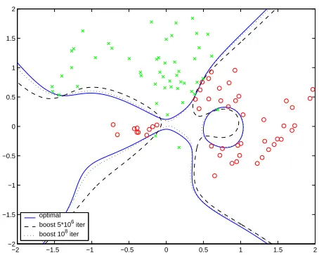
−2 −1.5 −1 −0.5 0 0.5 1 1.5 2 −2

−1.5 −1 −0.5 0 0.5 1 1.5 2

optimal boost 5*106 _iter boost 108 iter

Figure 11: Artificial data set with l2-margin maximizing separator (solid), and l2-boosting models

after 5∗106_{iterations (dashed) and 10}8_{iterations (dotted) using}ε_{=0.0001. We observe}

the convergence of the boosting separator to the optimal separator

We hope our results will help in better understanding how and why boosting works. It is an interest-ing and challenginterest-ing task to separate the effects of the different components of a boostinterest-ing algorithm:

• Loss criterion

• Dictionary and greedy learning method

• Line search / slow learning

and relate them to its success in different scenarios. The implicit l1 regularization in boosting

may also contribute to its success, as it has been shown that in some situations l1 regularization is

inherently superior to others (see Donoho et al., 1995).

An important issue when analyzing boosting is over-fitting in the noisy data case. To deal with over-fitting, R¨atsch et al. (2001b) propose several regularization methods and generalizations of the original AdaBoost algorithm to achieve a soft margin by introducing slack variables. Our results

indicate that the models along the boosting path can be regarded as l1 regularized versions of the

optimal separator, hence regularization can be done more directly and naturally by stopping the

boosting iterations early. It is essentially a choice of the l1constraint parameter c.

Many other questions arise from our view of boosting. Among the issues to be considered:

• Is there a similar “separator” view of multi-class boosting? We have some tentative results to

indicate that this might be the case if the boosting problem is formulated properly.

• Can the constrained optimization view of boosting help in producing generalization error

Acknowledgments

We thank Stephen Boyd, Brad Efron, Jerry Friedman, Robert Schapire and Rob Tibshirani for helpful discussions. We thank the referees for their thoughtful and useful comments. This work was partially supported by Stanford graduate fellowship, grant DMS-0204612 from the National Science Foundation, and grant ROI-CA-72028-01 from the National Institutes of Health.

Appendix A. Local Equivalence of Infinitesimalε-Boosting and l1-Constrained Optimization

As before, we assume we have a set of training data (x1,y1),(x2,y2), . . .(xn,yn), a smooth cost

function C(y,F), and a set of basis functions(h1(x),h2(x), . . .hJ(x)).

We denote by ˆβ(s)be the optimal solution of the l1-constrained optimization problem:

min β

n

∑

C(yi,h(xi)0β) (18)

subject to kβk1≤s. (19)

Suppose we initialize theε-boosting version of Algorithm 1, as described in Section 2, at ˆβ(s)and

run the algorithm for T steps. Letβ(T)denote the coefficients after T steps.

The “global convergence” Conjecture 2 in Section 4 implies that∀∆s>0:

β(∆s/ε)→βˆ(s+∆s) as ε→0

under some mild assumptions. Instead of proving this “global” result, we show here a “local” result

by looking at the derivative of ˆβ(s). Our proof builds on the proof by Efron et al. (2004, Theorem 2)

of a similar result for the case that the cost is squared error loss C(y,F) = (y−F)2_{. Theorem 1 below}

shows that if we start theε-boosting algorithm at a solution ˆβ(s)of the l1-constrained optimization

problem (18)–(19), the “direction of change” of theε-boosting solution will agree with that of the

l1-constrained optimization problem.

Theorem 1 Assume the optimal coefficient paths ˆβj(s) ∀j are monotone in s and the coefficient pathsβj(T)∀j are also monotone asε-boosting proceeds, then

β(T)−βˆ(s)

T·ε →∇βˆ(s) as ε→0,T →∞,T·ε→0.

Proof First we introduce some notations. Let

hj= (hj(x1), . . .hj(xn))0

be the jth basis function evaluated at the n training data. Let

F= (F(x1), . . .F(xn))0

be the vector of current fit. Let

r=

−∂C(y1,F1)

∂F1

, . . .−∂C(yn,Fn)

∂Fn

be the current “generalized residual” vector as defined in Friedman (2001). Let

cj=h0jr, j=1, . . .J

be the current “correlation” between hj and r.

Let

A

be the set of indices for the maximum absolute correlation.

For clarity, we re-write thisε-boosting algorithm, starting from ˆβ(s), as a special case of

Algo-rithm 1, as follows:

(1) Initializeβ(0) =βˆ(s),F0=F,r0=r.

(2) For t=1 : T

(a) Find jt=arg maxj|h0jrt−1|.

(b) Update

βt,jt ←βt−1,jt+ε·sign(cjt)

(c) Update Ft and rt.

Notice in the above algorithm, we start from ˆβ(s), rather than 0. As proposed in Efron et al. (2004),

we consider an idealized ε-boosting case: ε→0. As ε→0, T →∞ and T·ε→0, under the

monotone paths condition, Section 3.2 and Section 6 of Efron et al. (2004) showed

FT−F0

T·ε → u, (20)

rT−r0

T·ε → v, (21)

where u and v satisfy two constraints:

(Constraint 1) u is in the convex cone generated by{sign(cj)hj: j∈

A

u=

∑

Pjsign(cj)hj,Pj≥0.

(Constraint 2) v has equal “correlation” with sign(cj)hj,j∈

A:

sign(cj)h0jv=λA for j∈

A

The first constraint is true because the basis functions in

A

of|cj|for sufficiently small T·ε; the Pj’s are non-negative because the coefficient pathsβj(T)are

monotone. The second constraint can be seen by taking a Taylor expansion of C(y,F)around F0

to the quadratic term, letting T·εgo to zero and applying the result for the squared error loss from

Efron et al. (2004). Once the two constraints are established, we notice that

vi= − ∂2_C(y

i,F) ∂F2

F0(xi)

Hence we can plug the constraint 1 into the constraint 2 and get the following set of equations:

˜

H_ATW ˜H_AP=λ_A1,

where

˜

H_A = (· · ·sign(cj)hj· · ·), j∈

A

W = diag −∂

2_C(y i,F) ∂F2

F0(xi)

!

,

P = (· · ·Pj· · ·)0, j∈

A

If ˜H is of rank|A|(we will get back to this issue in details in Appendix B), then P, or equivalently

u and v, are uniquely determined up to a scale number.

Now we consider the l1-constrained optimization problem (18)–(19). Let ˆF(s) be the fitted

vector and ˆr(s)be the corresponding residual vector. Since ˆF(s)and ˆr(s)are smooth, define

u∗ ≡ lim

∆s→0

ˆ

F(s+∆s)−_Fˆ_(s)

∆s , (22)

v∗ ≡ lim

∆s→0

ˆr(s+∆s)−ˆr(s)

∆s . (23)

Lemma 2 Under the monotone coefficient paths assumption, u∗and v∗also satisfy constraints 1–2.

Proof Write the coefficientβjasβ+j −β−j, where

β+

j =βj,β−j =0 if βj>0, β+

j =0,β−j =−βj if βj<0.

The l1-constrained optimization problem (18)–(19) is then equivalent to

min

β+_,β−

n

∑

C yi,h(xi)0(β+−β−)

, (24)

subject to kβ+k1+kβ−k1≤s,β+≥0,β−≥0. (25)

The corresponding Lagrangian dual is

L = n

∑

C yi,h(xi)0(β+−β−)

+λ J

∑

(β+_j +β−_j) (26)

−λ·s−

J

∑

λ+

jβ+j − J

∑

λ−

jβ−j, (27)

whereλ≥0,λ+_j ≥0,λ−_j ≥0 are Lagrange multipliers.

By differentiating the Lagrangian dual, we get the solution of (24)–(25) needed to satisfy the following Karush-Kuhn-Tucker conditions:

∂L ∂β+

j