Linear Fractional Multi-Objective Optimization Problems Subject to Fuzzy Relational Equations with the Max-Average Composition

(1)

Published online February 6, 2015 (http://www.sciencepublishinggroup.com/j/acm) doi: 10.11648/j.acm.s.2015040102.15

ISSN: 2328-5605 (Print); ISSN: 2328-5613 (Online)

Linear fractional multi-objective optimization problems

subject to fuzzy relational equations with the max-average

composition

Z

.

Valizadeh-Gh

1, *

,

E

.

Khorram

2 1

Department of Mathematics , Roudehen Branch , Islamic Azad University , Roudehen , Iran 2

Faculty of Mathematics and Computer Science, Amirkabir University of Technology, Tehran , Iran

Email address:

[email protected] (Z . Valizadeh-Gh)

To cite this article:

Z . Valizadeh-Gh, E . Khorram. Linear Fractional Multi-Objective Optimization Problems Subject to Fuzzy Relational Equations with the Max-Average Composition. Applied and Computational Mathematics. Special Issue: New Advances in Fuzzy Mathematics: Theory, Algorithms, and Applications. Vol. 4, No. 1-2, 2015, pp. 20-30. doi: 10.11648/j.acm.s.2015040102.15

Abstract:

In this paper , linear fractional multi-objective optimization problems subject to a system of fuzzy relational equations (FRE) using the max-average composition are considered . First , some theorems and results are presented to thoroughly identify and reduce the feasible set of the fuzzy relation equations . Next , the linear fractional multi-objective optimization problem is converted to a linear one using Nykowski and Zolkiewski's approach . Then , the efficient solutions are obtained by applying the improved -constraint method . Finally , the proposed method is effectively tested by solving a consistent test problem .

Keywords

:

Fuzzy Relational Equation, The Max-Average Composition,

Linear Fractional Multi-Objective Optimization Problems, The Improved -Constraint Method

1. Introduction

Multi-objective programming problems play an important role in the optimization theory . Generally speaking , the objective functions of a multiple objective programming (MOP) problem may conflict with one another . Thus , the notion of Pareto optimality or efficiency associated with the feasible region has been introduced . There are several methods to find the efficient solutions of the MOP in the literature . For details see [6].

An optimization problem with multiple objective functions and fuzzy relational equation (FRE) or fuzzy relational inequality (FRI) constraints is among interesting issues in this field . Wang [23] considered a multi-objective mathematical programming problem with constraints defined by the FRE with the max-min composition . The nonlinear multi-objective optimization problems subject to FRE with the max-min and max-average compositions were studied in [16] and [13,14] , respectively . They developed specific reduction procedures to simplify a given problem , according to the special structure of the solution set , and further proposed some genetic algorithms to attain efficient

solutions . Many researchers have considered the problem and developed the theoretical topics , solution procedures and various applications [1-5,8-12,17,18,20,22,24-26].

Here , a linear fractional multi-objective optimization problem subject to the FRE with the max-average composition is considered . Since the feasible domain of this problem is generally non-convex , traditional methods may have difficulty in deriving the set of efficient solutions . Nevertheless, here, an efficient method is proposed to obtain the efficient solutions of the linear fractional multi-objective optimization problem (LFMOP) subject to the FRE, exactly and completely, using special structures of the feasible domain and the objective functions . Indeed, the linear fractional multi-objective optimization problem is converted to a linear one using Nykowski and Zolkiewski's approach [19] . Then , the efficient solutions are obtained by applying the improved -constraint method .

(2)

with fuzzy relation equation constraints. To illustrate the procedure , a numerical example will be provided in Section 5 that will be followed by our concluding remarks in Section 6.

2. Preliminaries

In this section , some definitions and theorems are presented which are basic in the literature [6]. Consider ,

min ∈ = = , … , (2.1)

where : ℛ ⟶ ℛ is a nonlinear vector function and ⊆

ℛ is the set of feasible solutions . Moreover , ∈ and =

∈ ℛ : ∃x ∈ χ, z = , … , ! are called a solution vector and the criterion space , respectively .

Notation 2.1. Let x, y ∈ ℛ# ,

≦ % ⟺ '≤ %', for ) = 1, … , +.

≤ % ⟺ ≦ % _and ≠ %. < % ⟺ '< %', for ) = 1, … , +.

Letz , z/∈ Z , we sayz dominatesz/andz is non-dominated if and only if z ≤ z/and there is no z ∈ Z that dominates z , respectively . Moreover , we say1 ∈ is an efficient solution to problem (2.1) if and only if there is no

x ∈ χ such that ≤ 1 .

In the remainder of the present section , some definitions , notations and theorems from different topics are reviewed which are needed in the latter sections . Let2 =

31, … , 45 ,6 = 31, … , +5 ,7 = 31, … , 85 , 9 = :;_<'=_{>× #} and

@ = @< >× , ;<', @<∈ [0,1], for all i ∈ I and j ∈ J. A system

of fuzzy relation equations with the max-average composition can be considered as

9GHI = @, (2.2)

where the operator “G_HI” is defined as follows :

;<GHI = max'∈KHLM_/N M, O ∈ 2, (2.3)

and ;_< is the i-th row of A.

Notation 2.2. For the i-th constraint (2.2) , we set

JQ = Rj ∈ J: a<' < 2bQU,

JQ/= Rj ∈ J: a<' = 2bQU,

JQV= Rj ∈ J: a<' > 2bQU,

X O = R) ∈ 6: 2@<− ;<' ≤ 1U, O ∈ 2

ℐ ) = 3O ∈ 2: ) ∈ X O 5, ) ∈ 6 χQ_{= 3 ∈ [0,1] : ;}

<GHI = @<5, O ∈ 2

= 3 ∈ [0,1] : 9GHI = @5.

and <are the feasible sets of the problem and the i-th constraint , respectively . When is not empty , it is in general

a non-convex and non-singleton set and can be completely determined by a unique maximum and a finite number of minimal solutions [21].

Definition 2.3. [15] . [ ∈ χ is a maximum solution if ≤

[ , for all ∈ , and if ≤ \ implies = \ , for all ∈ ,

\ ∈ is called a minimal solution .

Definition 2.4. [16]. If a value-change in some element(s) of a given fuzzy relation matrix 9 has no effect on the solutions of a corresponding fuzzy relation equations , this value-change is called an equivalence operation.

A traditional approach for solving the MOP is the scalarization techniques that formulate the MOP as a single objective program . Sometimes , the feasible set , , is limited by some new constraints related to objective functions of the MOP and/or some new variables introduced . Here , we utilize a well-known scalarization technique called the -constraint method which was improved by Ehrgott and Ruzika [7]. In this method , the corresponding single program to the MOP (2.1) is ,

min ] − ∑<a ]_<`<N+ ∑<a ]c<`<d

`. e.

< + `<N− `<d≤ <, O ∈ 7 ∖ 3g5

`<N,`<d≥ 0, O ∈ 7 ∖ 3g5

x ∈ χ,

(2.4)

where __<,c_<≥ 0 , for all O ∈ 7 ∖ 3g5.

The following results on the improved -constraint method can be found in [7]:

(i) If there is an O ≠ g such that c_<− __<< 0 , then problem (2.4) will be unbounded.

(ii) If c − _ ≥ 0 , then there is always an optimal solution of (2.4) such that `_<N`_<d= 0 , O ≠ g.

(iii) Let _, c ≧ 0 . If [, `̂N, `̂d is an optimal solution of (2.4) , then [ will be a weakly efficient solution of the MOP.

(iv) Let _, c ≧ 0. Let [, `̂N, `̂d be an optimal solution of (2.4) . If [is unique , then [will be a strictly efficient solution of the MOP.

(v) Let _, c > 0 . Let [, `̂N, `̂d be an optimal solution of (2.4) . Then , [ is an efficient solution of the MOP.

We shall assume throughout the paper that c − _ ≥ 0 , and

m, n and p stand for the number of constraints in system (2.2) , the dimension of solution vectors and the number of objective functions of problem (2.1) , respectively .

3. Systems of Fuzzy Relation Equations

Here, the feasible set of systems of fuzzy relation equations is characterized and the corresponding reduced problem will be investigated. It means we consider the characteristics of the solution set of (2.2) , when ∈

[0,1] , that is ,

9GHI = @,

∈ [0,1] , (3.1)

and attempt to simplify the problem by reducing the solution set . System (3.1) can also be considered as ;_<G_HI = @_< ,

(3)

is defined by (2.3) . The results which are proven in this section are our contributions .

3.1. Characterization of the Feasible Set

Proposition 3.1. A vector ∈ [0,1] fulfills the i-th constraint if and only if

∀ ) ∈ 6, ' ≤ 2@<− ;<',

∃ )l∈ 6, 'm = 2@<− ;<'m.

(3.2)

Lemma 3.2. If 6_<V≠ ∅ then <= ∅ .

Proof. Let )_l∈ 6_<V . By contraction , if ∈ < then according to (2.3) , _'≤ 2@_<− ;_<' , for all ) ∈ 6 . Thus ,

'm≤ 2@<− ;<'m < 0 .

Corollary 3.3. If <≠ ∅ then 6_<V= ∅ .

Lemma 3.4. [12]. Let <≠ ∅ . The maximum solution in

< _is <_[_{= : [}< _{, … , [}< _{= where [}<

'= min:2@<− ;<', 1= ,

for all ) ∈ 6 .

Proof. <[∈ was shown in [12]. By contraction , we prove that <[is the maximum solution of < . Let ∈

< _and ₎

l∈ 6 such that '_l> [< '_l= min:2@_O −

;<'m, 1 . Thus , 'm > 2@<− ;<'m or '_l> 1 (this case is

impossible , since _{'_l}∈ [0,1] . If _'_m > 2@_<− ;_<'_m , we have max_'∈K ;_<'+ _' > 2@_< that is ∉ < .

Notation 3.5. Let <\ ) = : \ )< , … , \ )< = where

) ∈ X O (see Notation 2.2) and

\ ) _] = x2@<− ;<', g = ),

0, g ≠ ),y

< _(3.3)

Lemma 3.6. [12]. Let <≠ ∅ .

a . For all ) ∈ X O , <\ ) is a minimal solution in <. b . <= ⋃_{'∈} <}{ \< , [< | .

Definition 3.7.

[ = minQ∈~ <[ (3.4)

\ = maxQ∈~ <\ • O (3.5)

where • = • 1 , … , • 4 and • O ∈ X O for all O ∈ 2 . Lemma 3.8. [12].

a . [ is the maximum solution of (3.1).

b . _l⊆ €• , where _l denotes the minimal solutions set of , €• = 3\ • ∶ • ∈ ƒ 5 and ƒ = X 1 × … × X 4 .

c . χ = ⋃ [\ • , []_„∈… , where ƒ = R• = :• 1 , … , • 4 =∶

• O ∈ X O ,O = 1, … , 4 U .

Lemma 3.9. If there is an O ∈ 2 such that 6_<V≠ ∅ then

= ∅ .

Proof. According to Lemma 3.2 , the proof is obvious . Theorem 3.10. = ⋂_Q∈~ < .

Proof. Let ƒ = R• = :• 1 , … , • 4 =∶ • O ∈ X O ,O =

1, … , 4U It is sufficient to prove two statements: (1) ⊆ ⋂_<∈‡ <and (2)⋂_<∈‡ <⊆ .

For (1):

∈ ⟺ ∈∪‰∈Š[\ • , []

⟺ ∃• ∈ ƒ,\ • ≤ ≤ [ ⟺ ∃• ∈ ƒ, ∀g ∈ 6, :\ • =_]= 4;_<∈‡ : \:• O =< ₌

] ≤ ]≤ [] = 4O+_<∈‡ <[]

⟺ ∃• ∈ ƒ, ∀g ∈ 6, ∀ O ∈ 2, \< _{:• O =}

]≤ ] ≤ [ <

]

⟺ ∃• ∈ ƒ, ∀g ∈ 6, ∀O ∈ 2,

x2@<− ;<], g = • O

0, otherwise ≤ ] ≤ min 2@<− ;<], 1 y

(3.6)

⟺ ∃• ∈ ƒ, ∀g ∈ 6, ∀O ∈ 2,

x2@<− ;<], g = • O

0, otherwise ≤ ] ≤ x2@₁_{, otherwise}<− ;<], g ∈ X O yy

⟺ ∀• ∈ 2, ∃• • ∈ X • , ∀g ∈ 6,∀O ∈ 2,

x2@<− ;<], g = • O

0, otherwisey ≤ ] ≤ x2@_{1, otherwise}<− ;<], g ∈ X O y

⟹ ∀• ∈ 2, ∃• • ∈ X • , Let ) = • • ,∀g ∈ 6,∀O = •,

x2@<− ;<], g = )

0, otherwisey ≤ ] ≤ x2@_{1, 2@}<− ;<] 2@<_<− ;_{− ;}<]_<]≤ 1 _{> 1}y

⟺ ∀O ∈ 2, ∃) ∈ X O , ∀g ∈ 6, \< ₎

]≤ ]≤ min 2@<− ;<], 1 = [ <

]

(3.7)

⟺ ∀O ∈ 2, ∃) ∈ X O , ∈ { \ )< _{, [}< _|

⟺ ∀O ∈ 2, ∈ • { \ )< _{, [}< _| '∈} <

⟺ ∀O ∈ 2, ∈ <

⟺ ∈ ‘ < <∈‡

For (2): Like to the previous part, we have:

x ∈ ‘ χQ Q∈~

⟺

⋯ ⟺ 3.7 ⟺ ∀O ∈ 2, ∃)<∈ X O , ∀g ∈ 6,

x2@<− ;<] , g = )<

0, otherwisey ≤ ]≤ x2@_{1, otherwise}<− ;<] , g ∈ X O y

⟺ ∀O ∈ 2, ∃)<= • O ∈ X O , ∀g ∈ 6,

x2@<− ;<] , g = • O

0, otherwisey ≤ ]≤ x2@_{1, otherwise}<− ;<] , g ∈ X O y

(4)

x2@<− ;<] , g = • O

0, otherwisey ≤ ] ≤ x2@_{1, otherwise}<− ;<] , g ∈ X O y

⟺ 3.6 ⟺ ⋯ ⟺ ∈

Remark 3.11. If @_<= 0 for some O ∈ 2 , it can be shown that

= ∅ .

According to Remark 3.11 and Lemma 3.9 , we shall assume in this section that @ > 0 and 6_<V= ∅ , for all O ∈

2 , respectively .

3.2. Problem Reduction

Detection of redundant constraints : Here , we consider the conditions under which a constraint of the problem can be omitted .

Theorem 3.12. Let ≠ ∅ , O , O_/∈ 2and O ≠ O_/ . If the O -th and O_/-th constraints satisfy

1 . X O = X O_/ ,

2 . ∀g ∈ X O = X O_/ , 2@_<_–− ;_<_–_] = 2@_<_—− ;_<_—_], then the constraint O_/ (or O ) is irredundent .

Proof. We show that⋂_QaQ_—χQ⊆ χQ—. Let ∈ ⋂_QaQ_—χQbe arbitrary .

∈ ‘ χQ QaQ—

⟺ ∀i ∈ I ∖ 3i/5, ∈ <= • { \ )< , [< | '∈} <

⟺ ∀O ∈ 2 ∖ 3i/5, ∃)<∈ X O , \ )< < ≤ ≤ [<

⟺ ∀O ∈ 2 ∖ 3O/5, ∃)<∈ X O ,∀g ∈ 6, : \ )< < =_]≤ ]≤ [< ]

⟺ ∀O ∈ 2 ∖ 3O/5, ∃)<∈ X O ,∀g ∈ 6,

x2@_{0, otherwise}<− ;<'L, g = )< y ≤ ]≤ [< ]= min 2@<− ;<], 1

⟺ ∀O ∈ 2 ∖ 3O/5, ∃)<∈ X O , ∀g ∈ 6,

˜ 0 ≤0 ≤ ]]≤ 1≤ 2@, <− ;<], g ∈ X O ∖ 3)g ∉ X O ,<5,

2@<− ;<'L ≤ ]≤ 2@<− ;<], g = )<

y

⟺ ∀O ∈ 2 ∖ 3O/5, ∃)<∈ X O ,

x _]]_{= 2@}≤ 2@_<<_{− ;}− ;_<'<], g ∈ X O ∖ 3)<5,

L, g = )<,

y

⟹ O = O , ∃)<– ∈ X O ,

™ ]≤ 2@<–− ;<–], g ∈ X O ∖ R)<–U, '_L–= 2@<–− ;<–'L–, g = )<–,

y

⟺ ∃)<– ∈ X O/ , ™ ]

≤ 2@<—− ;<—], g ∈ X O/ ∖ R)<–U, '_L–= 2@<—− ;<—'_L–, g = )<–,

y

⟺ ∃)<– ∈ X O/ , ∀g ∈ 6,

˜

0 ≤ ] ≤ 1, g ∉ X O/ ,

0 ≤ ] ≤ 2@<—− ;<—], g ∈ X O/ ∖ 3)<–5, '_L–= 2@<—− ;<—'L–, g = )<–,

y

⟺ ∃)<– ∈ X O/ ,∀g ∈ 6, : \:)<— <–==_]≤ ] ≤ [<— ]

⟺ ∈ • { \ )<— _{, [}<— _| '∈} <—

= <—

Example 3.13. Consider ,

š0.7954 0.4927 0.35470.7751 0.2369 0.8448

0.8165 0.5139 0.3759Ÿ GHI = š 0.6391 0.6289 0.6496Ÿ.

Here , we have X 1 = X 3 = 31,2,35 . Computing

<' = 2@<− ;<' , for all O ∈ 2 and ) ∈ 6 results that :

¡ = š0.4827 0.7854 0.92340.4827 1.0209 0.4130 0.4827 0.7854 0.9234Ÿ.

These values of the first and third rows are equal , thus , by applying Theorem 3.12 , the third (or the first) constraint is omitted . By solving the reduced system , we obtain the maximum solution ,[ = 0.4827,0.7854,0.4130 ¢and the minimal solutions as follows:

\: 1,1,1 = = 0.4827,0,0 £_,

\: 1,1,2 = = 0.4827,0.7854,0 £_,

\: 1,3,1 = = 0.4827,0,0.4130 £_.

Detection of fixed components : By the following lemmas , the j-th element of solutions can be fixed and be eliminated from the solution space .

Lemma 3.14. [12]. If for some ) ∈ 6 , <\ ) = 0• or ) ∈ 6_</ then the equation i has just one minimum as <\= 0• .

Lemma 3.15. For a constraint , say i , if 6_</≠ ∅ , then _'= 0 for all ∈ and all ) ∈ 6_</ . It means the component(s) j ,

) ∈ 6</ , can be eliminated from the solution space .

Proof. Let ∈ = ⋂_]∈‡ ] be arbitrary .

∈ ‘ ] ]∈‡

⟹ ∈ <

⟺ x∀) ∈ 6_{∃) ∈ 6,}, '≤ 2@<− ;<',

'= 2@<− ;<',y

⟹ ∀) ∈ 6</, '≤ 2@<− ;<' = 0,

⟹ ∀) ∈ 6</, '= 0.

Example 3.16. Consider the following feasible system

¤

0.2876 0.0912 0.5763 0.6834 0.5466

0.1917 0.7093

0.4258 0.1485 0.2363

0.6445 0.4579 0.1195

0.6477 0.7245 0.6073

¥ GHI = ¤

0.4214 0.4851 0.3622 0.5664 ¥

(5)

0.4236,0,0.2666,0 ¢_{, respectively .}

Lemma 3.17. Let ≠ ∅ . If there are O ∈ 2 and ) ∈ 6 such that @_<= ;_<' = 1 , then the j-th element of solutions can be fixed as one and be eliminated from the solution space .

Proof. We have:

χQ _{= 3x ∈ [0,1]}#_{: max}

¦∈§ aQ¦+ x¦ = 2bQ

= Rx ∈ [0,1]#_:_{∀k ∈ J}_,_a_Q¦_{+ x}_¦_{≤ 2}_{, ∃j}©_{∈ J}_,_a

Qª«+ x_ª«= 2U.

Since ;_<], _] ∈ [0,1] , for all g ∈ 6and ;_<'= 1 , the set < can be simplified as follows :

χQ_{= 3 x ∈ [0,1]}#_: _{let j}©_{= j a}_Qª_{+ x}_ª_{= 2 5}

= R x ∈ [0,1]#_:_x

ª= 2−aQª= 1 U

Example 3.18. Consider ,

š0.4425 1.0000 0.35930.7364 0.3948 0.6834

0.7041 0.4424 0.0197Ÿ 0HI = š 1.0000

0.8346 0.8185Ÿ

By Lemma 3.17, the second element of solutions can be fixed as one and be eliminated from the solution space , since

; /= @ = 1.0000 . The maximum and minimal solutions are [ = 0.9329,1.0000,0.9858 ¢ and

\ = 0.9329,1. 0000, 0¢_{, respectively .}

Lemma 3.19. Suppose X O = 3)_<5 (a singleton set) , for all

O ∈ 2 . If there is a )_l∈ 6 such that ℐ )_l ≠ ∅ (see Notation 2.2) , then

(1) 2@_<_m− ;_<_m_'_m = 2@_<_–− ;_<_–_'_m , for all O_l, O ∈ ℐ )_l . (2) for all ∈ , the )_l-th element of solutions can be fixed as 2@_<− ;_<'_m , O ∈ ℐ )_l , and the component )_l can be eliminated from the solution space .

Proof. (1) If ℐ )_l is singleton then O_l= O and the proof is trivial . Now , assume O_l, O ∈ ℐ )_l and O_l≠ O . Let =

, … , ∈ be an arbitrary feasible solution . We have :

max_ª∈§ :aQª + xª= = 2bQ i = il, i

⟺ ™_∃¬̅∀j ∈ J, aQª+ xª≤ 2bQ

Q ∈ J, a<®̅L+ x®̅L = 2bQ

y _{i = i}_l_{, i}

⟺ ˜∀j ∈ J\3jQ

5, xª ≤ 1 < 2bQ− aQª because j ∉ G i

j = jQ, xª≤ 2bQ− aQª≤ 1

∃¬̅Q∈ J, x®̅L = 2bQ− a<®̅L

y

i = il, i .

Therefore , it should be ¬̅_<= )_< , for O = O_l, O . On the other hand , by the assumption , we have )_<_m= )_<_– = )_l . Thus ,

'_Lm = '_L–= 'm , that is , 2@<m− ;<m'm = 2@<–− ;<–'m.

(2) By assumptions , the vector e is unique , • =

• 1 , … , • 4 = ) , … , )> . It is sufficient to prove

['= :\ • =_' :

['= :\ • =_'

⟺ min_Q∈~ <['= max_Q∈~ <\:• O = _' = max_Q∈~ <\ )_{< '}

⟺ min_Q∈~ :min:2bQ− aQª, 1== = max_Q∈~ x2b₀_{, otherwise}Q− aQª, j = jQ, _,y

⟺ min_{Q∈ℐ ª}:2bQ− aQª= = max_{Q∈ℐ ª}:2bQ− aQª=.

According to (1) , the last statement is true .

Example 3.20. Consider ,

š0.19490.1759 0.7701 0.11710.0602 0.0195

0.0773 0.9243 0.2973Ÿ GHI = š 0.6242 0.5635 0.7013Ÿ.

By computing 2@_<− ;_<' , for all i, j , we have X 1 = 325 ,

X 2 = 315 , X 3 = 325 , ℐ 1 = 325 , ℐ 2 = 31,35 and

ℐ 3 = 35 . By Lemma 3.19 , the first and second elements of solutions can be fixed as 0.9510 and

0.4782 , respectively , and can be eliminated from the solution space . The maximum and minimal solutions are [ = 0.9510,0.4782,1.0000 ¢ and

\ = 0.9510,0.4782,0 ¢_{, respectively.}

Corollary 3.21. If there is a ) ∈ 6 such that the values of

2@<− ;<' are equal for all O ∈ 2 , that is:

∃j ∈ J, ∀i , i/∈ I, 2bQ–− aQ–'= 2bQ—− aQ—',

then the j-th element of solutions can be fixed as 2@_<− ;_<' and be eliminated from the solution space .

According to this corollary , in Example 3.13 the first component of solutions can be fixed as 0.4827 and be eliminated from the solution space . Note that when omitting a column of the coefficient matrix causes a zero row , the corresponding constraint is redundant and should be eliminated from consideration .

Corollary 3.22. If 6_</≠ ∅ , for all O ∈ 2 and ⋃ 6_<∈‡ _</= 6 then

[ = \ = 0 . It means = 30•5 .

Identification of equivalence operation:

Corollary 3.23. [12]. When for some O ∈ 2and ) ∈ 6 ,

) ∉ X O , then the value of ;_<' has no effect on the solution space of (3.1) and can be changed to zero . In other words , changing ;_<'to zero is an equivalence operation (see Definition 2.4) .

Corollary 3.24. [12]. When for some ) ∈ 6and O , O_/∈ 2 ,

2@<–− ;<–'< 2@<—− ;<—' , then the value of ;<—' has no effect

on the solution space of (3.1) and can be changed to zero . In other words , changing ;_<_—_' to zero is an equivalence operation .

Proof. It is sufficient to prove ;_<_—_'+ _' < 2@_<_— , for all

∈ . Let ∈ be arbitrary . Since max_]∈K:;_<_—_]+ _]= =

2@<— , we have ;<—]+ ] ≤ 2@<— , for all g ∈ 6 , thus , ;<—'+ ' ≤ 2@<— . On the other hand , if ;<—'+ '= 2@<— , then

according to the assumption we have ;_<_–_'+ _' = ;_<_–_'+

2@<_/− ;<—'> 2@<– . Hence , max¦∈§:;<—]+ ]= ≥ ;<–M+ ' > 2@<– , which contradicts with ∈ <–and therefore ,

(6)

Example 3.25. Consider the following feasible system

š0.1382 0.50780.3844 0.6957 0.62790.8567

0.4504 0.4737 0.9497Ÿ GHI = š 0.7122 0.5978

0.7587Ÿ. (3.8)

Computing _<' = 2@_<− ;_<' , for all O ∈ 2 and ) ∈ 6 results in :

¡ = š1.2862 0.91660.8113 0.4999 0.56770.5677 1.0670 1.0438 0.5677Ÿ.

According to Corollary 3.23, changing ; , ;_V and ;_V/ to zero is an equivalenceoperation , since 1 ∉ X 1 = 32,35 ,

1 ∉ X 3 = 335$ and 2 ∉ X 3 . Additionally , by Corollary 3.24 , the value of ; _/has no effect on the solution space of (3.8) and can be changed to zero (since ¡_/= 0.9166 >

¡//= 0.4999) . Thus , the system converts to

š0.0000 0.00000.3844 0.6957 0.62790.8567

0.0000 0.0000 0.9497Ÿ GHI = š 0.7122

0.5978 0.7587Ÿ.

By solving the reduced system , we obtain the maximum solution ,

[ = 0.8113,0.4999,0.5677 £_,

and the minimal solutions as follows:

\: 3,1,3 = = 0.8113,0,0.5677 £_,

\: 3,2,3 = = 0,0.4999,0.5677 ¢_,

\: 3,3,3 = = 0,0,0.5677 ¢_.

4. Linear Fractional Multi-objective

Optimization Problems Subject to

Fuzzy Relational Equations

Here , we consider

min = ´µ–¶ ·–¶ , … ,

µ¸¶ ·¸¶¹

s. t. AoHIx = b

x ∈ [0,1]#

(4.1)

where 7_] = º_]£ + º_]l , »_] = ¼_]£ + ¼_]l , g = 1, … , 8 ,

8 ≥ 2 , º_]£ = º_] , … , º_] ∈ ℛ , ¼_]£ = ¼_] , … , ¼_] ∈ ℛ ,

º]l and ¼]l are two constant numbers and GHI is the

max-average composition . Using the improved -constraint method , we try to find the efficient solutions .

First , some assumptions and results are mentioned on the characteristic of (4.1) . We denote by ½ , the set of all efficient solutions of (4.1) , that is

½_{= 3 ̅ ∈ [0,1] :}_{∄ ∈} _, _≤ _{̅ 5}_,

which is non-empty regarding Assumptions 4.1 .

Assumptions 4.1. Let

1 . 7_] and »_] be continuous real valued functions on

= 3 ∈ [0,1] : 9G¿ = @5 .

2 . »_] be positive for all g ∈ 7 = 31, … , 85 and all ∈ . Clearly , the generality of the problem is not to be lost by this assumption .

3 . be a non-empty and compact set in ℛ .

4 . º_]£and¼_]£ be the k-th row of À = :º<'= _× and Á =

:¼<'= _× , respectively .

5 . Á ∈ [0,1] × and |À| = :Ãº_<'Ã= ∈ [0,1] × .

6 . À_l= :ºl, … , ºl= ∈ [−1,1] × and Á_l= :¼l, … , ¼l= ∈

[0,1] × _.

Definition 4.2. Problem (4.1) is called incomplete , if there is a g_l∈ 7 such that ¼_]£_m= 0• ∈ ℛ .

Definition 4.3. The objective functions of (4.1) are in conflict if l∩ _/l∩ … ∩ l= Å , where _]l , g = 1, … , 8, denotes the set of optimal solutions for the problem

min ] =Æ_ÈÇ_Ç : ∈ ,»] > 0!,

and is a nonempty and compact set in ℛ .

Now , we deal with Theorems 4.4 – 4.5 which are similar to those of Nykowski and Zolkiewski [19].

Theorem 4.4. Suppose ̅ ∈ ½ . 1 . If _] =Æ_ÈÇ

Ç > 0 , for all g ∈ 7 and all ∈ then

̅ ∈ É_where

É_{= argmin Γ} _{= 7} _{, … , 7} _{, −»} _{, … , −»} _{: ∈ !}

= 3 ̅ ∈ [0,1] : ∄ ∈ ,Γ ≤ Γ ̅ 5.

That is ½ ⊂ É . 2 . If _] =Æ_ÈÇ

Ç < 0 , for all g ∈ 7 and all ∈ then

̅ ∈ Í_{(that is} ½ _⊂ Í_{) where} Î_{= argmin}

RÏ = :7 , … , 7 , » , … , » =: ∈ U = 3 ̅ ∈ [0,1] : ∄ ∈ ,Λ ≤ Λ ̅ 5.

Proof. 1. Let ̅ ∉ É , that is , there is an _l∈ such that

Γ l ≤ Γ ̅ . Then , there is a non-negative vector ¼ ∈

ℛ/ _{such thatΓ ̅ = Γ}

l + ¼ . Thus ,

] ̅ =Æ_ÈÇ_Ç _̅̅ =_ÈÆ_{Ç m}Ç m_dÑNÑ_ÒÓÇÇ ≥_ÈÆÇ m_{Ç m} = ] l ,

g = 1, … , 8.

Additionally , there is an ` ∈ 7 such that ¼_Ô+ ¼ _NÔ>

0 , and _Ô ̅ > _{Ô l} . Therefore , ̅ ≥ _l , that is , ̅ ∉ ½ .

2 . Let ̅ ∉ Í , that is , there is an _l∈ such that Λ _l ≤

Λ ̅ . There is a non-negative vector ¼ ∈ ℛ/ such that

Λ ̅ = Λ l + ¼ . Thus , for g ∈ 7 ,

] ̅ =_»7] ̅ ] ̅ =

7] l + ¼]

»] l + ¼ N]≥

7] l

(7)

1

»] l + ¼ N]≤

1

»] l and 7] l < 0

⟹ _» 7] l

] l + ¼ N]≥

7] l

»] l .

Therefore ,

] ̅ ≥_» 7] l ] l + ¼ N]≥

7] l

»] l = ] l .

Similar to part (1) , it can be shown that ̅ ∉ ½which is a contradiction .

Theorem 4.5. Suppose ̅ ∈ ½ . If ] =Æ_ÈÇ_Ç > 0, for

g ∈ 31, … , ℎ5 and ] =Æ_ÈÇ_Ç < 0 , for g ∈ 3ℎ +

1, … , 85 (for all ∈ ) then ̅ ∈ × where

×_{= argmin3Φ : ∈ 5 = 3 ̅ ∈ [0,1] : ∄} _∈

, Φ ≤ Φ ̅ 5, where

Φ = 7 , … , 7 , −» , … , −»Ù , »ÙN , … , » .

That is ½ ⊂ × .

Proof. Let ̅ ∉ × , that is , there is an _l∈ such that

Φ l ≤ Φ ̅ . Thus , there is a non-negative vector ¼ ∈

ℛ/ _{such that}_{Φ ̅ = Φ}

l + ¼ . Similar to Theorem

4.4 , the proof can be completed .

Remark 4.6. Theorems 4.4 and 4.5 can also be applied on an incomplete linear fractional multi-objective problem .

Remark 4.7. According to the mathematical programming theory , some constant values can be added to each objective function in (4.1), with no effect on the optimal solutions set . This means that ;ÚÛ4O+RÜ = : +

¼ , … , + ¼ : ∈ U = ½ _where _{:¼ , … , ¼ = ∈}

ℛ . Therefore , we are always able to consider the equivalent MOP problem with positive objective functions on instead of the original problem (4.1) , using the following algorithm :

Algorithm 4.8.

1 . Given MOP (4.1) and let > 0 be a small user-defined scalar , say = 10dÝ .

2 . Define a constant vector Þ = :Þ , … , Þ = ∈ ℛ as follows :

Þ]= ˜

0, If _] > 0, GÚ all ∈ ,

−7ß]

»ß] + , otherwise,

y

where 7ß_] = min _∈ 7_] and »ß_] = min _∈ »_] , for

g ∈ 7 .

3 . The equivalent problem of (4.1) with positive objective functions on is

min ∈ Ü = : + Þ , … , + Þ =. (4.2)

Since there are finitely many objective functions 8 <

∞ , and in the course of the algorithm , two linear programming problems each with a single objective function are solved when there is an ∈ and a g ∈ 31, … , 85such

that _] < 0, Algorithm 4.8 terminates . Moreover , the following lemma shows the efficiency of Algorithm 4.8.

Lemma 4.9. The objective functions of (4.2) are positive on .

Proof. Consider an objective function _] and an _l∈ with _{] l} ≤ 0 . We show that _{] l} + Þ_]> 0 .

] l + Þ]= ] l +dÆß_Èß_ÇÇ+

= ] l +d áQ#_áQ#_ââ_ÈÆ_ÇÇ +

= ] l +áã¶_áQ#â:dÆ_â_È_ÇÇ =+

≥ ] l +−7_»] l ] l +

= ] l − ] l +

= > 0

Remark 4.10. By Theorem 4.4 , the linear multi-objective problem related to (4.2) is

min_∈ ä• = :7 + Þ » , … , 7 + Þ » ,y

y −» , … , −» = (4.3) and we have å⊆ É æ .

Assume that the FRE system (3.1) is simplified as much as possible by the results in Section 3. Let be the reduced feasible set . Using Assumption 4.1, problem (4.3) can be reformulated as

4O+ ∈ ä• = º£+ Þ ¼£ + ºl+ Þ ¼l , …, :º£+

Þ ¼£ _{+ :º}l_{+ Þ ¼}l_=, _{− ¼}£ _{− ¼}l_{, … , −¼}£ _{− ¼}l _._(4.4)

By omitting the constant values of the objective functions , we have

4O+ ∈ äç = º£+ Þ ¼£ , …, :º£+ Þ ¼£= , −

¼£ _{, … , −¼}£ _._(4.5)

Note that Éè= Éæ.

Now , we find Éèby applying the improved -constraint method (2.4) on problem (4.5) . Note that the set of efficient solutions of problem (4.1) , ½ , is a subset of Éè , i.e . ½⊆

Éè_⊆ _{. Hence , to obtain} ½_{, it is sufficient to solve the}

following problem on a smaller feasible set Éèinstead of :

min

∈ éè = = , … , .

Since Éèis a discrete set , a p dimension vector can be related to each individual of Éèin which the k-th element individually evaluates the k-th objective function . The efficient solutions can be obtained by comparing such vectors .

5. Numerical Testing

(8)

generated consistent constrained optimization problem .

min s. t. ê

0.4588 0.6620 0.7703 0.3503

0.6620 0.4162 0.8419 0.8329 0.2564 0.0106 0.4363 0.4273 0.8700 0.2649 0.3181 0.1193

ë GHI = ¤

0.5770 0.6786 0.4758 0.7826 ¥ ∈ [0,1]ì_,

,

where : ℛì→ ℛV , is defined as

=dl.ìÝlV _ Nl.î Ýì _/Nl. VVï _VNl.îÝìV _ìdl.ðïìV_{l.ÝVÝ/ _} _N_l.ñð _{_/Nl.ðï ì _V}_N_{l.ñVÝî _ìNl.îñïð},

/ =l.ïîñ _ dl.ðVññ _/dl./ìï/ _V_{l. ì} _{_ Nl.lVìî _/Nl. /î _VNl.îðì/ _ìNl.ì/ñî} dl.ïlð _ì dl.ñ/ñÝ ,

V =dl.ñ/Vî _ N_{l.ïV// _ Nl.ìÝÝð _/Nl.ïìV/ _V} l./Ýìï _/ dl.îïìð _Vdl.l/ ï _ìdl.l/ðî_N_{l.ìðÝñ _ìNl.lïñ/} .

First , according to results in Section 3, we reduce the feasible set of the problem as much as possible . According to Theorem 3.12 and Corollary 3.21, the redundant third and fourth constraints can be ignored and the first component of solutions is fixed to 0.6952 and this component can be eliminated from the solution space as well as the first column of the coefficient matrix from consideration . Thus , the constrained linear fractional optimization problem is reduced to

min ̅

s. t. 0.6620 0.7703 0.0000

0.0000 0.0000 0.8329 GHI = 0.5770 _0.6786

∈ [0,1]V_,

where the reduced objective function ̅: ℛV→ ℛV, is

̅ ₌ l.î Ýì _ Nl. VVï _/Nl.îÝìV _Vdl.ðïìV l.ñð _ Nl.ðï ì _/N l.ñVÝî _VNl.îñïð ,

̅

/ =dl.ðVññ _ dl./ìï/ _/dl.ïlð _V_{l.lVìî _ Nl. /î _/Nl.îðì/ _VNl.ì/ñî} dl.ñ/ñÝ ,

̅

V =l./Ýìï¶__{l.ìÝÝð¶_ Nl.ïìV/¶_/} dl.îïìð¶_/dl.l/ ï¶_Vdl.l/ðî_N_{l.ìðÝñ¶_VNl.lïñ/} .

The maximum solution and the minimal solutions of the feasible region are [ = 0.4920,0.3837,0.5243 £ , \ =

0.4920,0,0.5243 £ _and _\/₌

0,0.3837,0.5243 ¢ _{, respectively . Solving the problem}

following the method described in Section 4, it is concluded that

̅½_{= 31 = 0.4920,0.0000,0.5243} £_,y

y 1/_{= 0.0000,0.3837,0.5243} £_5,

̅ 1 = −0.3323, −1.9329,0.1715

and

̅ 1/ _{= −0.4835, −1.3997, −0.4199} _.

Therefore , by adding the first component of solutions with the value 0.6952 , the original solutions are obtained as

½_{= 31 = 0.6952,0.4920,0.0000,0.5243} £_,y

y1/_{= 0.6952,0.0000,0.3837,0.5243} £_5,

1 = −0.4091, −1.0945, −0.3075

and

1/ = −0.5116, −0.6457, −0.6140 .

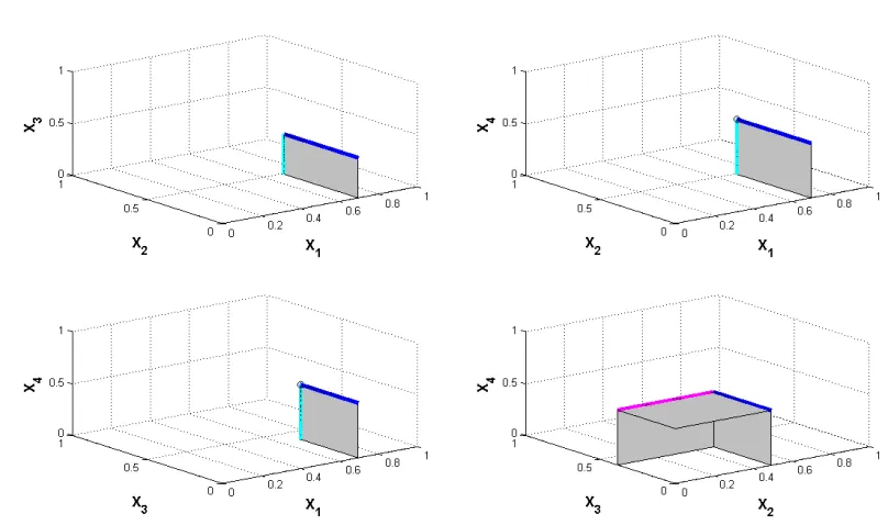
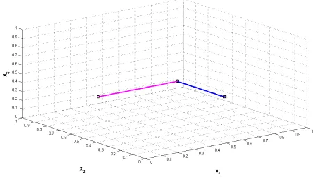
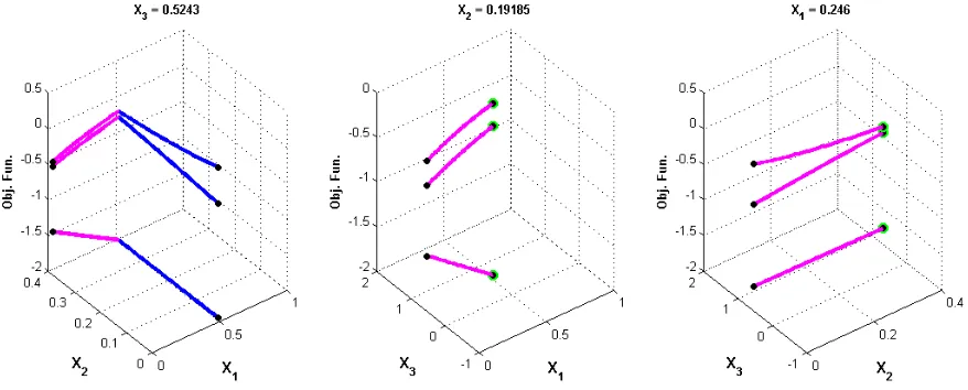
In Figures 1 and 2, different sections of the original feasible region and different sections of the original objective functions with the optimal solutions are shown , respectively . In addition , Figures 3 and 4 show different sections of the reduced feasible region and different sections of the reduced objective functions with the optimal solutions , respectively . The fixed variables and their values are shown in each figure .

(9)

Figure 2. The objective function and the optimal solutions of Example 5.1

(10)

Figure 4. The reduced objective function and the optimal solutions of Example 5.1

6. Conclusions

In this paper , we obtained the efficient solutions of linear fractional multi-objective optimization problems (LFMOP) subject to a system of fuzzy relational equations (FRE) using the max-average composition . First , some theorems and results were presented to thoroughly identify and reduce the feasible set of the FRE . Then , the LFMOP was converted to a linear multi-objective optimization problem using Nykowski and Zolkiewski's approach . Finally , the efficient solutions were obtained by applying the improved -constraint method . We tested the efficiency of the proposed method by solving a consistent test problem .

References

[1] Abbasi Molai, A., A new algorithm for resolution of the quadratic programming problem with fuzzy relation inequality constraints, Computers & Industrial Engineering, 72, 306-314 (2014)

[2] Abbasi Molai , A. , Resolution of a system of the max-product fuzzy relation equations using L○U-factorization , Information Sciences , 234 , 86--96 (2013)

[3] Abbasi Molai , A. , The quadratic programming problem with fuzzy relation inequality constraints , Computers & Industrial Engineering , 62(1) , 256--263 (2012)

[4] Brouwer , R.K. , A method of relational fuzzy clustering based on producing feature vectors using Fast Map , Information Sciences , 179(20) , 3561-3582 (2009)

[5] Di Martino , F. , & Sessa , S. , Digital watermarking in coding/decoding processes with fuzzy relation equations , Soft Computing , 10 , 238--243 (2006)

[6] Ehrgott , M. , Multicriteria Optimization , Springer , Berlin (2005)

[7] Ehrgott , M. , & Ruzika , S. , Improved -Constraint Method for Multiobjective Programming , Journal of Optimization Theory and Applications , 138 , 375--396 (2008)

[8] Friedrich , T. , Kroeger , T. , & Neumann , F. , Weighted preferences in evolutionary multi-objective optimization , International Journal of Machine Learning and Cybernetics , 4(2) , 139--148 (2013)

[9] Ghodousian , A. , & Khorram , E. , Linear optimization with an arbitrary fuzzy relational inequality , Fuzzy Sets and Systems , 206 , 89--102 (2012)

[10] Guo , F.F. , Pang , L.P. , Meng , D. , & Xia , Z.Q. , An algorithm for solving optimization problems with fuzzy relational inequality constraints , Information Sciences , 252 , 20-31 (2013)

[11] Guu , S.M. , Wu , Y.K. , & Lee , E.S. , Multi-objective optimization with a max-t-norm fuzzy relational equation constraint , Computers and Mathematics with Applications , 61 , 1559--1566 (2011)

[12] Khorram , E. , & Ghodousian , A. , Linear objective function optimization with fuzzy relation equation constraints regarding max-average composition , Applied Mathematics and Computation , 173 , 872--886 (2006)

[13] Khorram , E. , & Hassanzadeh , R. , Solving nonlinear optimization problems subjected to fuzzy relation equation constraints with max-average composition using a modified genetic algorithm , Computers & Industrial Engineering , 55 , 1--14 (2008)

[14] Khorram , E. , & Zarei , H. , Multi-objective optimization problems with fuzzy relation equation constraints regarding max-average composition , Mathematical and Computer Modelling , 49 , 856--867 (2009)

[15] Klir , G.J. , & Folger , T.A. , Fuzzy Sets , Uncertainty and information , Prentice-Hall , NJ (1988)

[16] Loetamonphong , J. , Fang , S.C. , & Young , R.E. , Multi-objective optimization problems with fuzzy relation equation constraints , Fuzzy Sets and Systems , 127 , 141--164 (2002) [17] Li , P. , & Fang , S.C. , Minimizing a linear fractional function

subject to a system of sup-T equations with a continuous Archimedean triangular norm , Journal of Systems Science and Complexity , 22 , 49--62 (2009)

(11)

[19] Nykowski , I. , & Zolkiewski , Z. , A compromise procedure for the multiple objective linear fractional programming problem , European Journal of Operational research , 19(1) , 91--97 (1985)

[20] Peeva , K. , Resolution of fuzzy relational equations Method , algorithm and software with applications , Information Sciences , 234 , 44--63 (2013) [21] Sanchez , E. , Resolution of composite fuzzy relation

equations , Information and Control , 30 , 38--48 (1976) [22] Sandri, S., & Martins-Bedê, F.T., A method for deriving order

compatible fuzzy relations from convex fuzzy partitions, Fuzzy Sets and Systems, 239, 91-103 (2014)

[23] Wang , H.F. , A multi-objective mathematical programming problem with fuzzy relation constraints , Journal of Multi-Criteria Decision Analysis , 4 , 23--35 (1995)

[24] Wang, X., Cao, X., Wu, C., & Chen, J., Indicators of fuzzy relations, Fuzzy Sets and Systems, 216, 91-107 (2013) [25] Wang, X., & Xue, Y., Traces and property indicators of fuzzy

relations, Fuzzy Sets and Systems, 246, 78-90 (2014) [26] Zhou , X.G. , & Ahat , R. , Geometric programming problem