Convolutional Nets and Watershed Cuts for Real-Time
Semantic Labeling of RGBD Videos
Camille Couprie [email protected]
IFP Energies Nouvelles
Technology, Computer Science and Applied Mathematics Division Rueil Malmaison, France
Cl´ement Farabet [email protected]
Twitter, Inc.
1355 Market St, Suite 900 San Francisco, CA 94103, USA
Laurent Najman [email protected]
Universit´e Paris-Est
Laboratoire d’Informatique Gaspard-Monge ´
Equipe A3SI - ESIEE Paris, France
Yann LeCun [email protected]
New York University & Facebook AI Research Courant Institute of Mathematical Sciences New York, NY 10003, USA
Editors:Aaron Courville, Rob Fergus, and Christopher Manning
Abstract
This work addresses multi-class segmentation of indoor scenes with RGB-D inputs. While this area of research has gained much attention recently, most works still rely on hand-crafted features. In contrast, we apply a multiscale convolutional network to learn features directly from the images and the depth information. Using a frame by frame labeling, we obtain nearly state-of-the-art performance on the NYU-v2 depth data set with an accuracy of 64.5%. We then show that the labeling can be further improved by exploiting the temporal consistency in the video sequence of the scene. To that goal, we present a method producing temporally consistent superpixels from a streaming video. Among the different methods producing superpixel segmentations of an image, the graph-based approach of Felzenszwalb and Huttenlocher is broadly employed. One of its interesting properties is that the regions are computed in a greedy manner in quasi-linear time by using a minimum spanning tree. In a framework exploiting minimum spanning trees all along, we propose an efficient video segmentation approach that computes temporally consistent pixels in a causal manner, filling the need for causal and real-time applications. We illustrate the labeling of indoor scenes in video sequences that could be processed in real-time using appropriate hardware such as an FPGA.
1. Introduction
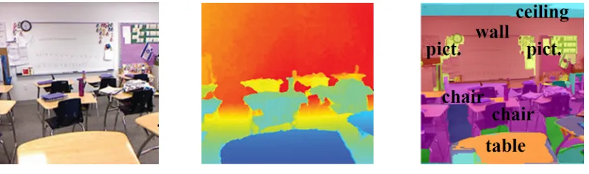
The recent release of the Kinect allowed for progress in indoor computer vision. Most approaches have focused on object recognition (Janoch et al., 2011) or point cloud semantic labeling (Koppula et al., 2009), finding their applications in robotics or games (Cruz et al., 2012). The pioneering work of Silberman and Fergus (2011) was the first to deal with the task of semantic full image labeling using depth information. This task implies the joint detection, recognition, and delineation at once (See Figure 1), closer to what our vision system perceives. Semantic segmentation results are still possible to improve, specifically in indoor environments where many objects may be similar, while belonging to different categories. Learning to segment full images in contrast to object recognition systems results in learning a context for the objects, such as co-occurrence relationships, that may help getting good results. Using RGB information, the deep learning approach of Farabet et al. (2013) achieves state-of-the-art semantic labeling performances while being an order of magnitude faster than competing approaches. In contrast with previous works employing hand-crafted features, the feature learning and the semantic predictions are performed using a unique model: a multiscale convolutional network, described in Section 2. The goal of this paper is to improve the result of this feature learning approach by using depth and temporal information, that is nowadays easily available in indoor environments.
Figure 1: From color and depth images, our goal is to predict semantic labels for the entire image, in other words, a semantic delineation of its components.
The first contribution of our work consists in adapting Farabet et al.’s network to learn more effective features for indoor scene labeling. Our work is, to the best of our knowledge, the first exploitation of depth information in a feature learning approach for full scene labeling (Couprie et al., 2013b).
including semantic segmentation as an application (Couprie et al., 2013a). We employ to that goal minimum spanning trees that are suitable to compute superpixels in quasi-linear time, therefore well adapted to real time applications.
The paper contains two main parts, the first dealing with feature learning using depth information, and the second dealing with the temporal smoothing approach. It is organized as follows. After presenting the related work on each parts, we introduce the algorithms employed in Section 2 for the two different aspects separately. We finally present in Section 3 our results using depth on images, independently from the temporal aspects, then introduce our temporal smoothing results independently from depth information, and combine the two aspects in the last results.
1.1 Related Work
Before detailing previous works on temporal smoothing methods, we introduce the existing background around depth-based segmentation approaches.
1.1.1 Learning To Segment Using Depth Information
The first results of Silberman and Fergus (2011) on the NYU depth data set employ sift features on the depth maps in addition to the RGB images. The depth is then used in the gradient information to refine the predictions using graph cuts. Alternative MRF-like approaches have also been explored to improve the computation time performance such as Couprie (2012). The results on NYU data set v1 have been improved by Ren et al. (2012) using elaborate kernel descriptors and a post-processing step that employs gPb superpixels MRFs, involving large computation times.
A second version of the NYU depth data set was released by Silberman et al. (2012), and improves the labels categorization into 894 different object classes. Furthermore, the size of the data set did also increase, it now contains hundreds of video sequences (407024 frames) acquired with depth maps. Recently, shortly after the submission of this paper, several groups designed features adapted to the NYU depth v2 data set, and present their results on the 4-class grouping of Silberman et al. (2012). M¨uller and Behnke (2014) use random forests averaging predictions within superpixels, but also explicitly learning interactions between neighboring superpixels using CRFs. They obtain state-of-the-art performance on NYU depth v2. The work of Cadena and Koˇsecka (2013) also uses handcrafted features and a CRF framework. Despite the better performance of these methods in comparison to our results, their computation times remain higher. Furthermore, the complexity of their inference constrains their methods to a low number of different classes to identify. The work of (St¨uckler et al., 2013), based on random decision forests and implemented on GPUs, is achieving fine performance in terms of speed and accuracy because it combines, like our work, depth and temporal information.
The present work aims at not only combining all available information (depth, spatial, and temporal consistency) to answer the challenging problem of indoor scene segmentation, but also avoiding the expense of designing data specific features.
prediction, object recognition (Hinton et al., 2012), mitosis detection (Ciresan et al., 2013) and many more applications. In computer vision, the approach of Farabet et al. (2012, 2013); Farabet (2014) has been specifically designed for full scene labeling and has proven its efficiency for outdoor scenes. The key idea is to learn hierarchical features by the mean of a multiscale convolutional network. Training networks using multiscale representations appeared also the same year in Ciresan et al. (2012); Schulz and Behnke (2012).
When the depth information was not yet available, there have been attempts to use stereo image pairs to improve the feature learning of convolutional networks as in LeCun et al. (2004). Now that depth maps are easy to acquire, deep learning approaches started to be considered for improving object recognition such as in Socher et al. (2012). Similarly, the work of Lenz et al. (2013) experiments group regularization to differentiate between the color and depth channels, treated as different modalities.
1.1.2 Temporal Smoothing
A large number of approaches in computer vision makes use of super-pixels at some point in the process, for example, semantic segmentation (Farabet et al., 2013), geometric con-text identification (Hoiem et al., 2005), extraction of support relations between object in scenes (Silberman et al., 2012), etc. Among the most popular approaches for super-pixel segmentation, two types of methods are distinguishable. Regular shape super-pixels may be produced using normalized cuts or graph cuts, see the works of Shi and Malik (1997); Veksler et al. (2010) for instance. More object—or part of object—shaped super-pixels can be generated from watershed based approaches. In particular, the method of Felzenszwalb and Huttenlocher (2004) produces such results.
It is a real challenge to obtain a decent delineation of objects from a single image. When it comes to real-time data analysis, the problem is even more difficult. However, additional cues may be used to constrain the solution to be temporally consistent, thus helping to achieve better results. Since many of the underlying algorithms are in general super-linear, there is often a need to reduce the dimensionality of the video. To this end, developing low level vision methods for video segmentation is necessary. Currently, most video processing approaches are non-causal, that is to say, they make use of future frames to segment a given frame, sometimes requiring the entire video as in (Grundmann et al., 2010). This prevents their use for real-time applications.
Some works (Glasner et al., 2011; Lee et al., 2005; Joulin et al., 2012; Gomila and Meyer, 2003; Xu et al., 2012) use the idea of enforcing some consistency between differ-ent segmdiffer-entations. Glasner et al. (2011) formulate a co-clustering problem as a Quadratic Semi-Assignment Problem. However solving the problem for a pair of images takes about a minute. Alternatively, Lee et al. (2005) and Gomila and Meyer (2003) identify the cor-responding regions using graph matching techniques. Xu et al. (2012) propose like us to exploit Felzenszwalb et al. superpixels in causal video processing. The complexity of this approach is super-linear because of a hierarchical segmentation, preventing the current im-plementation from real-time applications.
Our strategy to produce temporal superpixels is to perform independent segmentations and match the produced super-pixels to define markers. The markers are then used to produce the final segmentation by minimizing a global criterion defined on the image. We show how Minimum Spanning Trees can be used at every step of the process, leading to gains in speed, and real-time performance on a single core CPU.
2. Full Scene Labeling
We introduce in this section the employed feature learning approach from RGBD images, as well as our temporal smoothing methodology to improve the segmentation results on video.
2.1 Multi-Scale Feature Extraction
Good internal representations are compact, and fast to process. Multi-scale approaches such as hierarchies meet these requirements. In vision, pixels are assembled into edglets, edglets into motifs, motifs into parts, parts into objects, and objects into scenes. This suggests that recognition architectures for vision (and for other modalities such as audio and natural language) should have multiple trainable stages stacked on top of each other, one for each level in the feature hierarchy.
Convolutional Networks (ConvNets) provide a simple framework to learn such hierar-chies of features. Introduced by Fukushima (1980), they became usable thanks to LeCun et al. (1998) who proposed the first back-propagation algorithm. Riesenhuber and Poggio (1999) replaced Fukushima’s competition layers by max-pooling layers. Since the first GPU implementation of Ciresan et al. (2011), ConvNets have been used with GPUs in virtu-ally all non-recurrent, feedforward, competition-winning or benchmark record-setting deep learners (for object detection, image segmentation, traffic signs, ImageNet, Pascal).
F3
convnet
F1
F2
F
f1 (X1;𝛉1)
labeling l (F, h (I))
superpixels RGBD
Laplacian pyramid
g (I)
table wallceiling
chair chair pict. pict.
f3 (X3;𝛉3)
f2 (X2;𝛉2)
Input RGB image Input depth image
segmentation h (I)
Figure 2: Scene parsing (frame by frame) using a multiscale network and superpixels. The RGB channels of the image and the depth image are transformed through a Laplacian pyramid. Each scale is fed to a 3-stage convolutional network, which produces a set of feature maps. The feature maps of all scales are concatenated, the coarser-scale maps being upsampled to match the size of the finest-scale map. Each feature vector thus represents a large contextual window around each pixel. In parallel, a single segmentation of the image into superpixels is computed to exploit the natural contours of the image. The final labeling is obtained by the aggregation of the classifier predictions into the superpixels.
A great gain has been achieved with the introduction of the multiscale convolutional network described in Farabet et al. (2013). The multi-scale, dense feature extractor produces a series of feature vectors for regions of multiple sizes centered around every pixel in the image, covering a large context. The multi-scale convolutional net contains multiple copies of a single network that are applied to different scales of a Laplacian pyramid version of the RGBD input image.
The RGBD image is first pre-processed, so that local neighborhoods have zero mean and unit standard deviation. The depth image, given in meters, is treated as an additional channel similarly to any color channel. The overview scheme of our model appears in Figure 2.
Beside the input image which is now including a depth channel, the parameters of the multi-scale network (number of scales, sizes of feature maps, pooling type, etc.) are identical to Farabet et al. (2013). The feature maps sizes are 16, 64, 256, multiplied by the three scales. The size of convolutions kernels are set to 7 by 7 at each layer, and sizes of subsampling kernels (max pooling) are 2 by 2. In our tests we rescaled the images to the size 240×320.
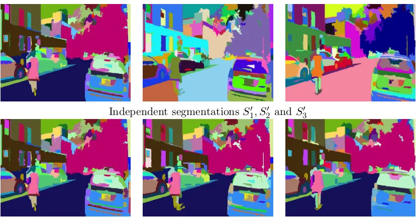
Independent segmentationsS10, S20 and S30
Temporally consistent segmentationsS1(=S01), S2, and S3
Figure 3: Segmentation results on three consecutive frames of the NYU-Scene data set.
ConvNet predictions as a post-processing step, by aggregating the classifiers predictions in each superpixel.
2.2 Movie Processing
While the training is performed on single images, we are able to perform scene labeling of video sequences. In order to improve the performance of our frame-by-frame predictions, a temporal smoothing may be applied. Instead of using the frame by frame superpixels as in the previous section, we compute temporally consistent superpixels. Our approach works in quasi-linear time and reduces the flickering of objects that may appear in the video sequences.
The temporal smoothing method presented in this section is introduced for RGB images and may trivially be extended to use depth information.
Given a segmentation St of an image at time t, we wish to compute a segmentation
St+1 of the image at time t+ 1 which is consistent with the segments of the result at time
t. For that purpose, we first compute a superpixel segmentation of the image at timet+ 1 using only this frame, and denote the resulting independent segmentation S0t+1, as detailed in Section 2.2.1.
2.2.1 Independent Image Segmentation
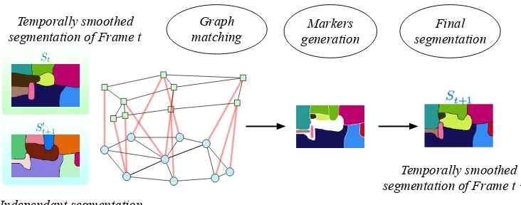
seg-Markers generation
Independant segmentation of Frame t +1 Temporally smoothed
segmentation of Frame t matchingGraph
St
S0
t+1
Final segmentation
Temporally smoothed segmentation of Frame t +1
Figure 4: Illustration of the temporal segmentation procedure
mentations S0
1, ..., ST0 , where T denotes the index of the last frame of the video sequence.
The principle of segmentation is fairly simple. We define a graphGt, where the nodes
cor-respond to the image pixels, and the edges link neighboring nodes in 8-connectivity. The edge weights ωij between nodes i and j are given by a color gradient of the image, or a
color and depth gradient if depth is available.
A Minimum Spanning Tree (MST) is build onGt, and regions are merged according to
a criterion taking into account the regions sizes and a scale parameterk. Once an image is independently segmented, resulting inS0
t+1, we then face the question of the propagation of the temporal consistency given the non overlapping contours of St
and St0+1. Our solution is the development of a cheap graph matching technique to obtain correspondences between segments from St and these of St0+1. This first step is described in Section 2.2.2. We then mine these correspondences to create markers (also called seeds) to compute the final labeling St+1 by solving a global optimization problem. This second step is detailed in Section 2.2.3.
2.2.2 Graph Matching Procedure
The basic idea is to use the segmentation St and segmentation St0+1 to produce markers before a final segmentation of image at timet+ 1. Therefore, in the process of computing a new segmentation St+1, a graph G is defined. The vertices of G comprise two sets of vertices: Vt that corresponds to the set of regions of St and Vt0+1 that corresponds to the set of regions of St0+1. Edges link regions characterized by a small distance between their centroids. The edges weights between vertex i∈Vt and j ∈Vt0+1 are given by a similarity measure taking into account distance and differences between shape and appearance
wij =
(|ri|+|rj|)d(ci, cj) |ri∩rj|
+aij, (1)
where |ri|denotes the number of pixels of regionri,|ri∩ rj|the number of pixels present
In our experiments aij was defined as the difference between mean color intensities of the
regions. It may also include depth information if available.
The graph matching procedure is illustrated in Figure 4 and produces the following result: For each region of St0+1, its best corresponding region in image St is identified.
More specifically, each node iof Vt is associated with the node j of Vt0+1 which minimizes
wij. Symmetrically, for each region of St, its best corresponding region in image St0+1 is identified, that is to say each node i of V0
t+1 is associated with the node j of Vt which
minimizeswij. This step may also be viewed as the construction of two minimum spanning
trees, one spanningVt, and the other Vt+1.
2.2.3 Final Segmentation Procedure
The final segmentationSt+1 is computed using a minimum spanning forest procedure. This seeded segmentation algorithm that produces watershed cuts as shown by Cousty et al. (2009) is strongly linked to global energy optimization methods such as graph-cuts as de-tailed by (All`ene et al., 2010; Couprie et al., 2011) and Section 2.3. In addition to theoretical guarantees of optimality, this choice of algorithm is motivated by the opportunity to reuse the sorting of edges that is performed in Section 2.2.1 and constitutes the main computa-tional effort. Consequently, we reuse here the graphGt+1(V, E) built for the production of independent segmentationS0
t+1.
Algorithm 1: Minimum Spanning Forest Algorithm
Data: A weighted graph G(V, E) and a set of labeled nodes makers L. Nodes of V \Lhave unknown labels initially.
Result: A labelingx associating a label to each vertex. Sort the edges ofE by increasing order of weight. while any node has an unknown label do
Find the edgeeij inE of minimal weight;
if vi or vj have unknown label values then
Mergevi and vj into a single node, such that when the value for this merged
node becomes known, all merged nodes are assigned the same value ofx and considered known.
The minimum spanning forest algorithm is recalled in Algorithm 1. The first appearance of such forest in image processing dates from 1986 with the work of Morris et al. (1986). It was later introduced in a morphological context by Meyer (1994).
The seeds, or markers, are defined using the regions correspondences computed in the previous section, according to the procedure detailed below. For each segment s0 of St0+1 four cases may appear:
1. s0 has one and only one matching region s inSt: propagate the label ls of region s.
All nodes ofs0 are labeled with the labell
s of region s.
2. s0 has several corresponding regions s
1, ..., sr: propagate seeds from St. The
coor-dinates of regions s1, ..., sr are centered on region s0. The labels of regions s1, ..., sr
3. s0 has no matching region : The region is labeled by the label l0
s itself.
4. If none of the previous cases is fulfilled, it means that s0 is part of a larger region s in St. If the size of s0 is small, a new label is created. Otherwise, the label ls is
propagated ins0 as in case 1.
Before applying the minimum spanning forest algorithm, a safety test is performed to check that the map of produced markers does not differ two much from the segmentation St0+1. If the test shows large differences, an eroded map of St0+1 is used to correct the markers. The eroded regions in the conflict areas are added as markers.
2.3 Global Optimization Guarantees
The minimum spanning forest computation offers by definition a global optimality guaran-tee, the sum of the edges weights of the forest being maximal. In addition, less commonly known, there is a probabilistic interpretation (as continuous Markov random fields) of the labeling of a particular case of such forests.
Several graph-based segmentation problems, including minimum spanning forests, graph cuts, random walks and shortest paths have recently been shown to belong to a common energy minimization framework, see the work of (All`ene et al., 2010; Sinop and Grady, 2007; Couprie et al., 2011). The considered problem is to find a labelingx∗ ∈
R|V|defined on the
nodes of a graph that minimizes
E(x) = X
eij∈E
wijp|xj−xi|q+
X
vi∈V
wpi|li−xi|q, (2)
where l represents a given configuration and x represents the target configuration. The result of limp→∞arg minxE(x) for values of q ≥ 1 always produces a cut by maximum
(equivalently minimum) spanning forest. The reciprocal is also true if the weights of the graph are all different.
In the case of our application, the pairwise weights wij is given by an inverse function
of the original weights ωij. The pairwise term thus penalizes any unwanted high-frequency
content inxand essentially forcesxto vary smoothly within an object, while allowing large changes across the object boundaries. The second term enforces fidelity of x to a specified configurationl,wi being the unary weights enforcing that fidelity.
The enforcement of markers ls—defined as described in Section 2.2.3 according to four
cases—as hard constrained may be viewed as follows: A node of label ls is added to the
graph, and linked to all nodes iof V that are supposed to be marked. The unary weights ωi,ls are set to arbitrary large values in order to impose the markers.
2.3.1 Applications To Optical Flow And Semantic Segmentation
An optical flow map may be easily estimated from two successive segmentations St and
St+1. For each region r of St+1, if the label of r comes from a label present in a region
s of the segmentation St, the optical flow in r is computed as the distance between the
region tracking applications. In principle, a video sequence will not contain displacements of objects greater than a certain value.
For each superpixel sof St+1, if the label of region s comes from the previous segmen-tation St, then the semantic prediction from St is propagated to St+1. Otherwise, in case the label of s is a new label, the semantic prediction is computed using the prediction at time t+ 1. As some errors may appear in the regions tracking, labels of regions having inconsistent large values in optical flow maps are not propagated. For the specific task of semantic segmentation, results can be improved by exploiting the contours of the recognized objects. Semantic contours such as for example transition between a building and a tree for instance, might not be present in the gradient of the raw image. Thus, in addition to the pairwise weights ω described in Section 2.2.1, we add a constant in the presence of a semantic contour.
3. Results
We used for our experiments the NYU depth data set—version 2—of Silberman et al. (2012), composed of 407024 couples of RGB images and depth images. Among these images, 1449 frames have been labeled. The object labels cover 894 categories. The data set is provided with the original raw depth data that contain missing values, with code from Dani et al. (2004) to inpaint the depth images.
3.1 Validation Of Our RGBD Network On Images
The training has been performed using the 894 categories directly as output classes. The frequencies of object appearances have not been changed in the training process. However, we established 14 clusters of classes categories to evaluate our results more easily. The distributions of number of pixels per class categories are given in Table 1. We used the train/test splits as provided by the NYU depth v2 data set, that is to say 795 training images and 654 test images. Please note that no jitter (rotation, translations or any other transformation) was added to the data set to gain extra performances. However, this strategy could be employed in future work. The code consists of Lua scripts using the Torch machine learning software of Collobert et al. (2011) available online at http://www.
torch.ch/.
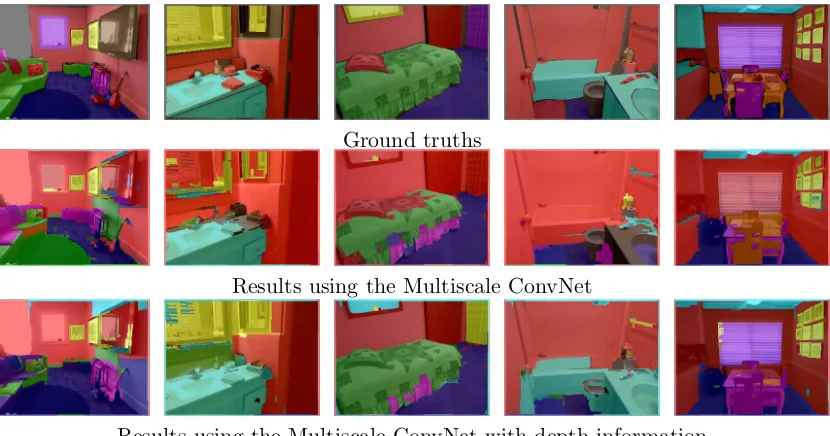
Ground truths
Results using the Multiscale ConvNet
Results using the Multiscale ConvNet with depth information
wall bed
books ceiling
chair floor
furniture pict./deco
sofa table
object window
TV uknw
Ground truths
Depth maps
Results using the Multiscale Convnet
Results using the Multiscale Convnet with depth information
• the “classwise accuracy”, counting the number of correctly classified pixels divided by the number of false positive, averaged for each class. This number corresponds to the mean of the confusion matrix diagonal.
• the “pixelwise accuracy”, counting the number of correctly classified pixels divided by the total number of pixels of the test data.
We tested to scale the depth image with a log scale, however it did not improved the results. We observe that considerable gains (15% or more) are achieved for the classes ’floor’, ’ceiling’, and ’furniture’. This result is logical since these classes are characterized by a globally constant appearance of their depth map. Objects such as TV, table, books can either be located in the foreground as well as in the background of images. On the contrary, the floor and ceiling will almost always lead to a depth gradient always oriented in the same direction: Since the data set has been collected by a person holding a Kinect device at a his chest, floors and ceiling are located at a distance that does not vary to much through the data set. Figure 5 provides examples of depth maps that illustrate these observations. Large drops of performances when using depth information are also observed for some classes (chair, table, window, books and TV). We explain this result partly by the very weak frequency of appearance of such classes in the data set that is not sufficient to cover the variety of possible depth appearance for these objects. One should also note that for specific applications, object frequencies may be weighted in the training step as in Farabet et al.’s work. Overall, improvements induced by the depth information exploitation are present and statistically significant, as checked using paired t-tests. In the next section, these improvements are more apparent.
3.2 Comparison to the State-Of-The-Art
In order to compare our results to the state-of-the-art on the NYU depth v2 data set, we adopted a different selection of outputs instead of the 14 classes employed in the previous section. The work of Silberman et al. (2012) defines the four semantic classes Ground, Furniture, Props and Structure. This class selection is adopted by Silberman et al. (2012) to use semantic labelings of scenes to infer support relations between objects. We recall that the recognition of the semantic categories is performed by (Silberman et al., 2012) using the definition of diverse features including SIFT features, histograms of surface normals, 2D and 3D bounding box dimensions, color histograms, and relative depth.
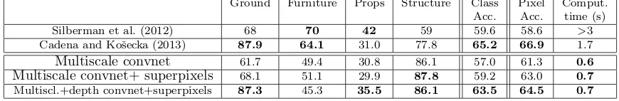
As reported in Table 2, the results achieved using the Multiscale convnet are improving the structure class predictions, resulting in an overall 4% relative gain in pixelwise accuracy over Silberman et al.’s approach. Adding the depth information results in a considerable improvement of the ground prediction, and better performance over the other classes. This approach achieves a 4% relative gain in classwise accuracy over previous works and improves by almost 6% the pixelwise accuracy compared to Silberman et al.’s results.
Class Multiscale Convnet Acc. MultiScale Convnet Occurrences Farabet et al. (2013) +depth Acc.
bed 4.4% 30.3 38.1
objects 7.1 % 10.9 8.7
chair 3.4% 44.4 34.1
furnit. 12.3% 28.5 42.4
ceiling 1.4% 33.2 62.6
floor 9.9% 68.0 87.3
deco. 3.4% 38.5 40.4
sofa 3.2% 25.8 24.6
table 3.7% 18.0 10.2
wall 24.5% 89.4 86.1
window 5.1% 37.8 15.9
books 2.9% 31.7 13.7
TV 1.0% 18.8 6.0
unkn. 17.8% -
-Avg. Class Accuracy - 35.8 36.2
Pixel Acc. (mean) - 51.0 52.4
Pixel Acc. (median) - 51.7 52.9
Pixel Acc. (std. dev.) - 15.2 15.2
Table 1: Class occurrences in the test set—Performance per class and per pixel. Results in bold indicate statistically significant better performances (above probability of 95% being statistically different)
Ground Furniture Props Structure Class Pixel Comput. Acc. Acc. time (s) Silberman et al. (2012) 68 70 42 59 59.6 58.6 >3 Cadena and Koˇsecka (2013) 87.9 64.1 31.0 77.8 65.2 66.9 1.7
Multiscale convnet 61.7 49.4 30.8 86.1 57.0 61.3 0.6
Multiscale convnet+ superpixels 68.1 51.1 29.9 87.8 59.2 63.0 0.7 Multiscl.+depth convnet+superpixels 87.3 45.3 35.5 86.1 63.5 64.5 0.7
Table 2: Accuracy of the multiscale convnet compared to the state-of-the-art. The reported computation times of Cadena and Koˇsecka (2013) were obtained on an architecture similar to ours. Bold numbers indicate the best or second best performance.
Very recently, the approach of Cadena and Koˇsecka (2013) achieved about two percent improvement over our results. Contrary to our system, they use handcrafted features, resulting therefore in a less versatile method.
details. The temporal smoothing only requires an additional 0.1s per frame, as we develop in the next section.
3.3 Super-Pixel Segmentation On Videos Using RGB Information
Next experiments demonstrate the efficiency and versatility of our temporal smoothing approach by performing simple super-pixel segmentation and semantic scene labeling.
Original frames Mean shift results of Paris (2008) Our results
Figure 6: Comparison of our temporal superpixels with the mean-shift segmentation method of Paris (2008) on Frame 19 and 20. k= 200, δ= 400, σ= 0.5.
Experiments are performed on two different types of videos: videos where the camera is static, and videos where the camera is moving. The robustness of our approach to large variations in the region sizes and large movements of camera is illustrated in Figure 7, where the camera is moving.
A comparison with the temporal mean shift segmentation of Paris (2008) is displayed in Figure 6. The super-pixels produced by Paris (2008) are not spatially consistent as the segmentation is performed in the feature (color) space in their case. Our approach is slower, although qualified for real-time application, but computes only spatially consistent super-pixels.
3.4 Semantic Video Labeling
Input images (frames 4 and 5) and difference image
Independent segmentationsS0
4, S50 (left) and temporally consistent segmentationsS4, S5 (right)
Figure 7: Segmentation results on 2 consecutive frames of the NYU-Scene data set.
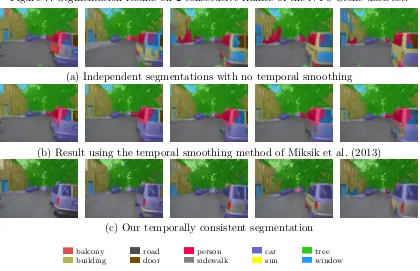
(a) Independent segmentations with no temporal smoothing
(b) Result using the temporal smoothing method of Miksik et al. (2013)
(c) Our temporally consistent segmentation
balcony building
road door
person sidewalk
car sun
tree window
Figure 8: Comparison with the temporal smoothing method of Miksik et al. (2013). Pa-rameters used: k= 1200, δ= 100, σ= 1.2.
3.4.1 Outdoor Segmentation Results
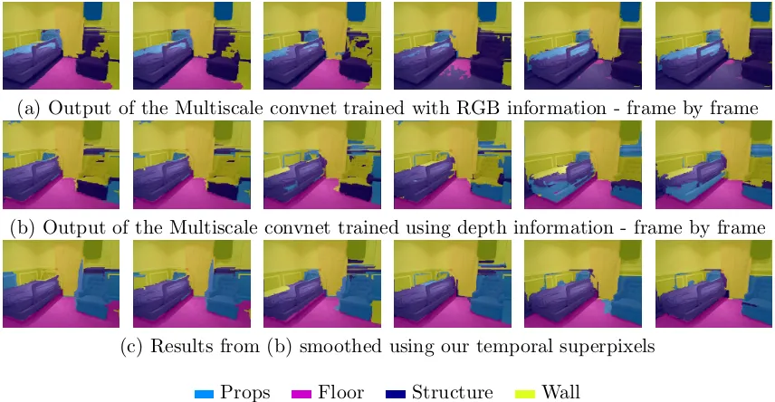
(a) Output of the Multiscale convnet trained with RGB information - frame by frame
(b) Output of the Multiscale convnet trained using depth information - frame by frame
(c) Results from (b) smoothed using our temporal superpixels
Props Floor Structure Wall
Figure 9: Some results on video sequences of the NYU v2 depth data set.
with the results of Miksik et al. (2013) on the NYU-Scene data set. The data set consists in a video sequence of 73 frames provided with a dense semantic labeling and ground truths. The provided dense labeling being performed with no temporal exploitation, it suffers from sudden large object appearances and disappearances. As illustrated in Figure 8 our ap-proach reduces this effect, and improves the classification performance of more than 5% as reported in Table 3.
Multiscale RGBD Convnet Temporal smoothing of Our temporal
Frame by frame Miksik et al. (2013) smoothing
Accuracy 71.11 75.31 76.27
#Frames/sec 1.43 1.33∗ 10.5
Table 3: Overall pixel accuracy (%) for the semantic segmentation task on the NYU Scene video and computation times ∗Note that the reported timing does not take into account the optical flow computation needed by Miksik et al. (2013).
3.4.2 Indoor Segmentation Results
Multiscale Multiscale convnet Multiscale convnet
convnet + depth + depth + temp. smoothing
dining room 54.5 63.8 58.5
living room 63.6 65.4 72.1
classroom 52 56.5 58.3
office 58.8 56.3 57.4
mean 57.2 60.5 61.6
Table 4: Overall pixel accuracy (%) for the semantic segmentation task on the NYU Depth data set. Parameter used for the temporal smoothing: δ = 100, σ = 1.2, k = 800,1000,1000,920.
The results obtained in Table 4 show that in most videos scenes, our temporal superpixels allow us to obtain better results. An example of results appears in Figure 9.
3.5 Computation Time of the Temporal Smoothing Approach
The experiments were performed on a laptop with 2.3 GHz Intel core i7-3615QM. Our method is implemented on CPU only, in C/C++, and makes use of only one core of the processor. Super-pixel segmentations take 0.1 seconds per image of size 320×240 and 0.4 seconds per image of size 640×380, thus demonstrating the scalability of the pipeline. All computations are included in the reported timings. The mean segmentation time using the work of Xu et al. (2012) for a frame of size 320×240 is 4 seconds. The timings of the temporal smoothing method of Miksik et al. (2013) are reported in Table 3. We note that the processor used for the reported timings of Miksik et al. (2013) has similar characteristics as ours. Furthermore, Mistik et al. use an optical flow procedure that takes only 0.02 seconds per frame when implemented on GPU, but takes seconds on CPU. Our approach is thus more adapted to real-time applications for instance on embedded devices where a GPU is often not available. The code, as well as some data and videos are available at the website of Couprie (2013).
4. Discussion and Conclusion
This works combines two independent contributions devoted to improve scene labeling re-sults. It introduces the addition of depth information into feature trainable architectures, which brings, for a 4-class segmentation task, a class accuracy improvement of more than 7% relatively to the training using only RGB data. The speed of our system is mainly allowed by the multiscale nature and the sparse connectivity of the employed convolutional network, allowing us to parse an image in 0.7s on CPU.
instance, poorly represented classes in the data set do not allow our model to sense the variability of the objects with the additional depth dimension.
In terms of evaluation, the 4-class split was designed for a specific application: to perform inference on support relationships between objects, but we deplore that all systems now use it for general purpose semantic labeling with depth. Indeed, it does not give insight about how well the concurrent systems discriminate objects in a world more complex than with four object categories.
With the temporal smoothing strategy, we demonstrate the ability of minimum spanning trees to fulfill accuracy and competitive timing requirements in a global optimization frame-work. Unlike many video segmentation techniques, our algorithm is causal and does not require any computation of optical flow. Our experiments on challenging videos show that the obtained super-pixels are robust to large camera or objects displacements. Their use in semantic segmentation applications demonstrate that significant gains can be achieved and lead to state-of-the-art results.
Our feature learning and temporal smoothing approaches were developed independently from each other, this presents the advantages of possibly being used in different appli-cations, and also having real time capabilities by decorrelating temporal aspects in the post-treatment. However the best approach for us would be to combine them in one fully trainable system, which will probably be possible in a near future with nowadays hardware computational advances.
Acknowledgments
We would like to thank Nathan Silberman for his useful input for handling the NYU depth v2 data set, and fruitful discussions.
References
C´edric All`ene, Jean-Yves Audibert, Michel Couprie, and Renaud Keriven. Some links between extremum spanning forests, watersheds and min-cuts. Image and Vision
Com-puting, 28(10):1460–1471, 2010.
C´esar Cadena and Jana Koˇsecka. Semantic parsing for priming object detection in RGB-D scenes. In3rd Workshop on Semantic Perception, Mapping and Exploration, 2013.
Dan Claudiu Ciresan, Ueli Meier, Jonathan Masci, Luca Maria Gambardella, and J¨urgen Schmidhuber. Flexible, high performance convolutional neural networks for image clas-sification. In Proc. of the 22nd International Joint Conference on Artificial Intelligence, pages 1237–1242, 2011.
Dan Claudiu Ciresan, Alessandro Giusti, Luca Maria Gambardella, and J¨urgen Schmidhu-ber. Deep neural networks segment neuronal membranes in electron microscopy images.
Dan Claudiu Ciresan, Alessandro Giusti, Luca Maria Gambardella, and J¨urgen Schmidhu-ber. Mitosis detection in breast cancer histology images using deep neural networks. In
MICCAI, 2013.
R. Collobert, K. Kavukcuoglu, and C. Farabet. Torch7: A Matlab-like environment for machines learning. InNIPS Big Learning Workshop, Sierra Nevada, Spain, 2011.
Dorin Comaniciu and Peter Meer. Mean shift: A robust approach toward feature space analysis. IEEE Trans. Pattern Analysis and Machine Intelligence, 24:603–619, 2002.
Camille Couprie. Multi-label energy minimization for object class segmentation. In 20th
European Signal Processing Conference, Bucharest, Romania, August 2012.
Camille Couprie. Source code for causal graph-based video segmentation, 2013.www.esiee.
fr/~coupriec/code.html.
Camille Couprie, Leo J. Grady, Laurent Najman, and Hugues Talbot. Power watershed: A unifying graph-based optimization framework. IEEE Trans. Pattern Analysis and
Machine Intelligence, 33(7):1384–1399, 2011.
Camille Couprie, Cl´ement Farabet, Yann LeCun, and Laurent Najman. Causal graph-based video segmentation. In Proc. of IEEE International Conference on Image Processing, 2013a.
Camille Couprie, Cl´ement Farabet, Laurent Najman, and Yann LeCun. Indoor semantic segmentation using depth information. In International Conference on Learning
Repre-sentations, 2013b.
Jean Cousty, Gilles Bertrand, Laurent Najman, and Michel Couprie. Watershed cuts: Minimum spanning forests and the drop of water. IEEE Trans. Pattern Analysis and
Machine Intelligence, 31(8):1362–1374, 2009.
Leandro Cruz, Djalma Lucio, and Luiz Velho. Kinect and RGBD images: Challenges and applications. SIBGRAPI Tutorial, 2012.
Anat Levin Dani, Dani Lischinski, and Yair Weiss. Colorization using optimization. ACM
Transactions on Graphics, 23:689–694, 2004.
Cl´ement Farabet. Towards Real-Time Image Understanding with Convolutional Networks. PhD thesis, Universit´e Paris Est, 2014.
Clement Farabet, Camille Couprie, Laurent Najman, and Yann LeCun. Scene Parsing with Multiscale Feature Learning, Purity Trees, and Optimal Covers. InProc. of International
Conference on Machine Learning, Edinburgh, Scotland, June 2012.
Clement Farabet, Camille Couprie, Laurent Najman, and Yann LeCun. Learning hierarchi-cal features for scene labeling.IEEE Trans. on Pattern Analysis and Machine Intelligence, 35(8):1915–1929, Aug 2013.
Kunihiko Fukushima. Neocognitron: A self-organizing neural network model for a mecha-nism of pattern recognition unaffected by shift in position. Biological Cybernetics, 36(4): 193–202, 1980.
Daniel Glasner, Shiv Naga Prasad Vitaladevuni, and Ronen Basri. Contour-based joint clustering of multiple segmentations. In Proc. of IEEE Computer Vision and Pattern
Recognition, pages 2385–2392, Washington, DC, USA, 2011.
Cristina Gomila and Fernand Meyer. Graph-based object tracking. In Proc. of IEEE
International Conference on Image Processing, 2003.
Matthias Grundmann, Vivek Kwatra, Mei Han, and Irfan Essa. Efficient hierarchical graph-based video segmentation. In Proc. of IEEE Computer Vision and Pattern Recognition, 2010.
Geoffrey E. Hinton, Nitish Srivastava, Alex Krizhevsky, Ilya Sutskever, and Ruslan Salakhutdinov. Improving neural networks by preventing co-adaptation of feature de-tectors. CoRR, abs/1207.0580, 2012.
Derek Hoiem, Alexei A. Efros, and Martial Hebert. Geometric context from a single image.
InProc. of IEEE International Conference on Computer Vision, volume 1, pages 654–661,
2005.
Navdeep Jaitly, Patrick Nguyen, Andrew Senior, and Vincent Vanhoucke. Application of pretrained deep neural networks to large vocabulary speech recognition. In Proc. of
Interspeech, 2012.
Allison Janoch, Sergey Karayev, Yangqing Jia, Jonathan T. Barron, Mario Fritz, Kate Saenko, and Trevor Darrell. A category-level 3-D object dataset: Putting the kinect to work. In IEEE International Conference on Computer Vision Workshops, pages 1168– 1174, 2011.
Armand Joulin, Francis Bach, and Jean Ponce. Multi-class cosegmentation. In Proc. of
IEEE Computer Vision and Pattern Recognition, pages 542–549, 2012.
Hema S. Koppula, Abhishek Anand, Thorsten Joachims, and Ashutosh Saxena. Cornell-RGBD-dataset, 2009. http://pr.cs.cornell.edu/sceneunderstanding/data/data.
php.
Yann LeCun, Leon Bottou, Yoshua Bengio, and Patrick Haffner. Gradient-based learning applied to document recognition. Proc. of the IEEE, 86(11):2278 –2324, nov 1998.
Yann LeCun, Fu-Jie Huang, and Leon Bottou. Learning Methods for generic object recogni-tion with invariance to pose and lighting. InProc. of IEEE Computer Vision and Pattern
Recognition, 2004.
J. Lee, JungHwan Oh, and Sae Hwang. Clustering of video objects by graph matching. In
Ian Lenz, Honglak Lee, and Ashutosh Saxena. Deep learning for detecting robotic grasp, corr abs/1301.3592s. In Robotics: Science and Systems, 2013.
Fernand Meyer. Minimum spanning forests for morphological segmentation. In Proc. of
International Symposium on Mathematical Morphology, pages 77–84, 1994.
Ondrej Miksik, Daniel Munoz, J. Andrew Bagnell, and Martial Hebert. Efficient tempo-ral consistency for streaming video scene analysis. In Proc. of the IEEE International
Conference on Robotics and Automation, Karlsruhe, Germany, 2013.
O.J. Morris, M. de Jersey Lee, and A.G. Constantinides. Graph theory for image analysis: an approach based on the shortest spanning tree. Communications, Radar and Signal
Processing, IEE Proceedings F, 133(2):146–152, April 1986.
Andreas C M¨uller and Sven Behnke. Learning depth-sensitive conditional random fields for semantic segmentation of RGB-D images. InIEEE International Conference on Robotics
and Automation, Hong Kong, May, 2014.
Sylvain Paris. Edge-preserving smoothing and mean-shift segmentation of video streams.
In Proc. of IEEE European Conference on Computer Vision, pages 460–473, Marseille,
France, 2008.
Xiaofeng Ren, Liefeng Bo, and D. Fox. RGB-(D) scene labeling: Features and algorithms.
In Proc. of IEEE Conference on Computer Vision and Pattern Recognition, pages 2759
–2766, june 2012.
Maximilian Riesenhuber and Tomaso Poggio. Hierarchical models of object recognition in cortex. Nature Neuroscience, 2:1019–1025, 1999.
Hannes Schulz and Sven Behnke. Learning object-class segmentation with convolutional neural networks. In 11th European Symposium on Artificial Neural Networks, 2012.
Jianbo Shi and Jitendra Malik. Normalized cuts and image segmentation. In IEEE Trans.
on Pattern Analysis and Machine Intelligence, volume 22, pages 888–905, 1997.
Nathan Silberman and Rob Fergus. Indoor scene segmentation using a structured light sensor. In 3DRR Workshop, IEEE International Conference on Computer Vision
Work-shops, 2011.
Nathan Silberman, Derek Hoiem, Pushmeet Kohli, and Rob Fergus. Indoor segmentation and support inference from RGBD images. In Proc. of IEEE European Conference on
Computer Vision, 2012.
Ali Kemal Sinop and Leo Grady. A seeded image segmentation framework unifying graph cuts and random walker which yields a new algorithm. In Proc. of International
Confer-ence of Computer Vision, 2007.
Richard Socher, Brody Huval, Bharath Bhat, Christopher D. Manning, and Andrew Y. Ng. Convolutional-Recursive Deep Learning for 3D Object Classification. In Advances
J¨org St¨uckler, Benedikt Waldvogel, Hannes Schulz, and Sven Behnke. Dense real-time mapping of object-class semantics from RGB-D video. Journal of Real-Time Image
Pro-cessing, pages 1–11, 2013.
Olga Veksler, Yuri Boykov, and Paria Mehrani. Superpixels and supervoxels in an energy optimization framework. In Proc. of IEEE European Conference on Computer Vision,
Heraklion, Crete, Greece, September 5-11 (5), pages 211–224, 2010.
Chenliang Xu, Caiming Xiong, and Jason J. Corso. Streaming hierarchical video segmen-tation. In Proc. of IEEE European Conference on Computer Vision, Florence, Italy,