Robust Submodular Observation Selection

Robust Submodular Observation Selection

Andreas Krause [email protected]

Computer Science Department Carnegie Mellon University 5000 Forbes Ave.

Pittsburgh, PA 15213

H. Brendan McMahan [email protected]

Google, Inc. 4720 Forbes Ave. Pittsburgh, PA 15213

Carlos Guestrin [email protected]

Computer Science Department and Machine Learning Department Carnegie Mellon University

5000 Forbes Ave. Pittsburgh, PA 15213

Anupam Gupta [email protected]

Computer Science Department Carnegie Mellon University 5000 Forbes Ave.

Pittsburgh, PA 15213

Editor: Chris Williams

Abstract

Keywords: observation selection, experimental design, active learning, submodular functions, Gaussian processes

1. Introduction

In tasks such as sensor placement for environmental monitoring or experimental design, one has to select among a large set of possible, but expensive, observations. In environmental monitoring, we can choose locations where measurements of a spatial phenomenon (such acidicity in rivers and lakes, cf., Figure 1(a)) should be obtained. In experimental design, we frequently have a menu of possible experiments which can be performed. Often, there are several different objective functions which we want to simultaneously optimize. For example, in the environmental monitoring prob-lem, we want to minimize the marginal posterior variance of our acidicity estimate at all locations simultaneously. In experimental design, we often have uncertainty about the model parameters, and we want our experiments to be informative no matter what the true parameters of the model are. In sensor placement for contamination detection in water distribution networks (cf., Figure 1(b)), we want to place sensors in order to quickly detect any possible contamination event.

Our goal in all these problems is to select observations (sensor locations, experiments) which are robust against a worst-case objective function (location to evaluate predictive variance, model parameters, contamination event, etc.). Often, the individual objective functions, for example, the marginal variance at one location, or the information gain for a fixed set of parameters (Das and Kempe, 2008; Krause et al., 2007b; Krause and Guestrin, 2005; Guestrin et al., 2005), satisfy

sub-modularity, an intuitive diminishing returns property: Adding a new observation helps less if we

have already made many observations, and more if we have made few observation thus far. While NP-hard, the problem of selecting an optimal set of k observations maximizing a single submodular objective can be approximately solved using a simple greedy forward-selection algorithm, which is guaranteed to perform near-optimally (Nemhauser et al., 1978). However, as we show, this sim-ple myopic algorithm performs arbitrarily badly in the case of a worst-case objective function. In this paper, we address the fundamental problem of nonmyopically selecting observations which are robust against such an adversarially chosen submodular objective function. In particular:

• We present SATURATE, an efficient algorithm for the robust submodular observation selection problem. Our algorithm guarantees solutions which are at least as informative as the optimal solution, at only a slightly higher cost.

• We prove that our approximation guarantee is the best possible, that is, the guarantee cannot be improved unless NP-complete problems admit efficient algorithms.

• We discuss several extensions of our approach, handling complex cost functions and trading off worst-case and average-case performance.

• We extensively evaluate our algorithm on several real-world tasks, including minimizing

the maximum posterior variance in Gaussian Process regression, finding experiment designs which are robust with respect to parameter uncertainty, and sensor placement for outbreak detection.

SATURATE, an efficient approximation algorithm for this problem (Section 4), and show that our ap-proximation guarantees are best possible, unless NP-complete problems admit efficient algorithms (Section 5). In Section 6, we discuss how many important machine learning problems are instances of our robust submodular observation selection formalism. We then discuss extensions (Section 7) and evaluate the performance of SATURATE on several real-world observation selection problems (Section 8). Section 9 presents heuristics to improve the computational performance of our algo-rithm, Section 10 reviews related work, and Section 11 presents our conclusions.

(a) NIMS deployed at UC Merced (b) Water distribution network

Figure 1: (a) Deployment of the Networked Infomechanical System (NIMS, Harmon et al., 2006) to monitor a lake near UC Merced. (b) Illustration of the municipal water distribution network considered in the Battle of the Water Sensor Networks challenge (cf., Ostfeld et al., 2008).

2. Robust Submodular Observation Selection

In this section, we first review the concept of submodularity (Section 2.1), and then introduce the

robust submodular observation selection (RSOS) problem (Section 2.2).

2.1 Submodular Observation Selection

Let us consider a spatial prediction problem, where we want to estimate the pH values across a horizontal transect of a river, for example, using the NIMS robot shown in Figure 1(a). We can discretize the space into a finite number of locations

V

, where we can obtain measurements, and model a joint distribution P(

X

V)over variables

X

V associated with these locations. One example of such models, which have found common use in geostatistics (cf., Cressie, 1991), are Gaussian Processes (cf., Rasmussen and Williams, 2006). Based on such a model, a typical goal in spatial monitoring is to select a subset of locations

A

⊆

V

to observe, such that the average predictive variance,

V(

A

) = 1

is minimized (cf., Section 6.1 for more details). Hereby, σ2_i|A denotes the predictive variance at location i after observing locations

A

, that is,

σ2 i|A=

Z

P(x_A)E

(

X

i−E[

X

i|xA])2|xA

dx_A.

Unfortunately, the problem

A

∗=argmin

|A|≤k V(

A

)

is NP-hard in general (Das and Kempe, 2008), and the number of candidate solutions is very large, so generally we cannot expect to efficiently find the optimal solution. Fortunately, as Das and Kempe (2008) show, in many cases, the variance reduction

Fs(

A

) =σ2s−σ2s|A

at any particular location s, satisfies the following diminishing returns behavior: Adding a new observation reduces the variance at s more, if we have made few observations so far, and less, if we have already made many observations. This formalism can be formalized using the combinatorial concept of submodularity (cf., Nemhauser et al., 1978):

Definition 1 A set function F : 2V →Ris called submodular, if for all subsets

A

,

B

⊆

V

it holds that F(

A

∪

B

) +F(

A

∩

B

)≤F(

A

) +F(

B

).

Nemhauser et al. (1978) prove a convenient characterization of submodular functions: F is submodular if and only if for all

A

⊆

B

⊆

V

and s∈

V

\

B

it holds that F(

A

∪{s})−F(

A

)≥F(

B

∪

{s})−F(

B

). This characterization exactly matches our diminishing returns intuition about the variance reduction Fsat location s. Since each of the variance reduction functions Fsis submodular,

the average variance reduction

F(

A

) =V(/0)−V(

A

) = 1

n

∑

_s Fs(

A

)

is also submodular. The average variance reduction is also monotonic, that is, for all

A

⊆

B

⊆

V

it holds that F(

A

)≤F(

B

), and normalized (F(/0) =0).

Hence, the problem of minimizing the average variance is an instance of the problem

max

A⊆VF(

A

), subject to |

A

| ≤k, (1)

where F is normalized, monotonic and submodular, and k is a bound on the number of observations we can make. As Krause and Guestrin (2007a) show, many other observation selection problems are instances of Problem (1).

Since solving Problem (1) is NP-hard in most interesting instances (Feige, 1998; Krause et al., 2006, 2007b; Das and Kempe, 2008), in practice, heuristics are often used. One such heuristic is the greedy algorithm. This algorithm starts with the empty set, and iteratively adds the element

s∗=argmax_s∈V\AF(

A

∪ {s}), until k elements have been selected. Perhaps surprisingly, a

Theorem 2 (Nemhauser et al. 1978) In the case of any normalized, monotonic submodular

func-tion F, the set

A

Gobtained by the greedy algorithm achieves at least a constant fraction(1−1/e) of the objective value obtained by the optimal solution, that is,

F(

A

G)≥(1−1/e)max |A|≤kF(

A

).

Moreover, no polynomial time algorithm can provide a better approximation guarantee unless P= NP (Feige, 1998).

2.2 The Robust Submodular Observation Selection (RSOS) Problem

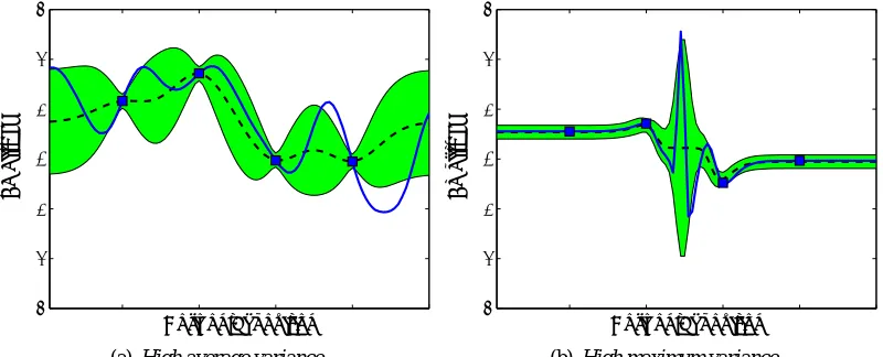
For phenomena, such as the one indicated in Figure 2(a), which are spatially homogeneous (isotropic), maximizing this average variance reduction leads to effective variance reduction everywhere in the space. However, many spatial phenomena are nonstationary, being smooth in certain areas and highly variable in others, such as the example indicated in Figure 2(b). In such a case, maximizing the average variance reduction will typically put only few examples in the areas highly variable areas. However, those regions are typically the most interesting, since they are most difficult to predict. In such cases, we might want to simultaneously minimize the variance everywhere in the space.

−3

−2

−1 0 1 2 3

Horizontal position

Amplitude

(a) High average variance

−3

−2

−1 0 1 2 3

Horizontal position

Amplitude

(b) High maximum variance

Figure 2: Spatial predictions using Gaussian Processes with a small number of observations. The blue solid line indicates the unobserved latent function, and blue squares indicate observa-tions. The plots also show confidence bands (green). Dashed line indicates the prediction. (b) shows an example with high maximum predictive variance, but low average variance, whereas (a) shows an example with high average variance, but lower maximum variance. Note, that in (b) we are most uncertain about the most variable (and interesting, since it is hard to predict) part of the curve, suggesting that the maximum variance should be optimized.

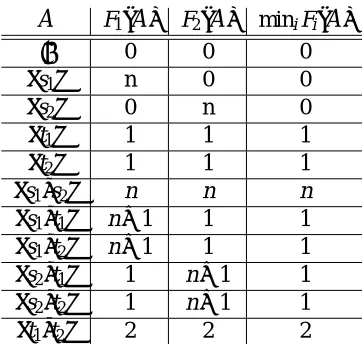
A

F1(

A

) F2(

A

) miniFi(

A

)

/0 0 0 0

{s1} n 0 0

{s2} 0 n 0

{t1} 1 1 1

{t2} 1 1 1

{s1,s2} n n n {s1,t1} n+1 1 1 {s1,t2} n+1 1 1 {s2,t1} 1 n+1 1 {s2,t2} 1 n+1 1 {t1,t2} 2 2 2

Table 1: Functions F1and F2used in the counterexample.

normalized monotonic submodular functions F1,...,Fm, and we want to solve

max

A⊆Vmini Fi(

A

), subject to |

A

| ≤k. (2)

The goal of Problem (2) is to find a set

A

of observations, which is robust against the worst possible objective, miniFi, from our set of possible objectives. Consider the spatial monitoring setting for

example, and assume that the prior varianceσ2_i is constant (we will relax this assumption in Sec-tion 7.2) over all locaSec-tions i. Then, the problem of minimizing the maximum variance, as motivated by the example in Figure 2, is equivalent to maximizing the minimum variance reduction, that is, solving Problem (2) where Fi is the variance reduction at location i.

We call Problem (2) the Robust Submodular Observation Selection (RSOS) problem. Note, that even if the Fi are all submodular, Fwc(

A

) =miniFi(

A

) is generally not submodular. In fact,

we show below that, in this setting, the simple greedy algorithm (which performs near-optimally in the single-criterion setting) can perform arbitrarily badly. While the example in Table 1 might seem artificial, as we show in Section 8 (especially Section 8.3), the greedy algorithm exhibits very poor performance when applied to practical problems.

3. Hardness of the Robust Submodular Observation Selection Problem

Given the near-optimal performance of the greedy algorithm for the single-objective problem, a nat-ural question is if the performance guarantee generalizes to the more complex robust optimization setting. Unfortunately, this hope is far from true, even in the simpler case of modular (additive) functions Fi. Consider a case with two submodular functions, F1and F2, where the set of

observa-tions is

V

={s1,s2,t1,t2}. The functions take values as indicated in Table 1. Optimizing for a set

of 2 elements, the greedy algorithm maximizing Fwc(

A

) =min{F1(

A

),F2(

A

)}would first choose t1(or t2), as this choice increases the objective min{F1,F2}by 1, as opposed to 0 for s1and s2. The

greedy solution for k=2 would then be the set{t1,t2}, obtaining a score of 2. However, the optimal

solution with k=2 is{s1,s2}, with a score of n. Hence, as n→∞, the greedy algorithm performs

Given that the greedy algorithm performs arbitrarily badly, our next hope would be to obtain a different good approximation algorithm. However, we can show that most likely this is not possible:

Theorem 3 Unless P=NP, there cannot exist any polynomial time approximation algorithm for

Problem (2). More precisely: If there exists a positive functionγ(·)>0 and an algorithm that, for

all n and k, in time polynomial in the size of the problem instance n, is guaranteed to find a set

_A

of size k such that miniFi(

A

)≥γ(n)max_|A|≤kminiFi(

A

), then P=NP.

Thus, unless P=NP, there cannot exist any algorithm which is guaranteed to provide, for example, even an exponentially small fraction (γ(n) =2−n) of the optimal solution. All proofs can be found in the Appendix.

4. The Submodular Saturation Algorithm

We now present an algorithm that finds a set of observations which perform at least as well as the optimal set, but at slightly increased cost; moreover, we show that no efficient algorithm can provide better guarantees (under reasonable complexity-theoretic assumptions).

4.1 Algorithm Overview

For now we assume that all Fitake only integral values; this assumption is relaxed in Section 7.1.

The key idea is to consider the following alternative problem formulation:

max

c,A c, subject to Fi(

A

)≥c for 1≤i≤m and|

A

| ≤k. (3)

We want a set

A

of size at most k, such that Fi(

A

)≥c for all i, and c is as large as possible. Note

that Problem (3) is equivalent to the original Problem (2): Maximizing c subject to the existence of a set

A

,|

A

| ≤k such that Fi(

A

)≥c for all i is equivalent to maximizing miniFi(

A

).

Now suppose we had an algorithm that, for any given value c, solves the following optimization problem:

A

c=argmin

A |

A

|

subject to Fi(

A

)≥c for 1≤i≤m (4)

that is, finds the smallest set

_A

with Fi(

A

)≥c for all i. If this set has at most k elements, then c (and

the set

A

) is feasible for the RSOS Problem (3). If we cannot find a set

A

satisfying Fi(

A

)≥c for

all i and containing at most k elements, then c is infeasible. A binary search on c would then allow us to find the optimal solution with the maximum feasible c. We call Problem (4) the MINCOVERc

problem, as it requires to find the smallest set guaranteeing an equal amount of coverage, c, for all objective functions Fi.

Since Theorem 3 rules out any approximation algorithm which respects the constraint k on the size of the set

A

, our only hope for non-trivial guarantees requires us to relax this constraint. Our algorithm is based on the following approach:

• We define a relaxed version of the RSOS problem with a superset of feasible solutions that

we call RELRSOS.

0 min_iF_i(V) c

c_max c_min

feasible c for RSOS

feasible c for RelRSOS search interval

c* c’

Figure 3: Illustration of feasible regions for the RSOS and RELRSOS problems. [cmin,cmax]is

the search interval during some iteration of SATURATE. c∗is the optimal solution to the

RSOS problem, and cis the solution that will eventually be returned by SATURATE.

• We will then successively improve the upper and lower bounds using a binary search

pro-cedure. Upon convergence, we are thus guaranteed a feasible solution to RELRSOS, that

performs at least as well as the optimal solution to the RSOS problem.

We now define the RELRSOS problem, the relaxed version of the RSOS Problem (3).

max

c,A c, subject to Fi(

A

)≥c for 1≤i≤m and|

A

| ≤αk. (5)

Hereby, α ≥1 is a parameter relaxing the constraint on |

A

|. If α=1, we recover the RSOS Problem (3).

As described above, our goal will be to approximately solve the RELRSOS Problem (5) for a fixed constantα. More formally, we will develop an efficient algorithm, SATURATE, which returns

a solution(c,

A

) that is feasible for the RELRSOS Problem (5), and achieves a score that is at least as good as an optimal solution(c∗,

A

∗)to the RSOS Problem (3), that is, c≥c∗and|

A

| ≤

α|

A

∗| ≤αk.

The basic idea of SATURATEis to use the binary search procedure (maintaining a search interval

[cmin,cmax]) as described above, but using an approximate algorithm, GPC (for Greedy Partial Cov-erage) that we will develop below, for the MINCOVER_c Problem (4). When invoked with a fixed value c, the GPC algorithm will return a feasible solution|

A

c| to the MINCOVERcProblem (4). We

will furthermore guarantee that

• |

A

c|>αk implies that c>c∗, that is, c is an upper bound to the RSOS Problem (3), and

hence it is safe to set cmax=c, and

• |

A

c| ≤αk implies that

A

c is a feasible solution (lower bound) to the RELRSOS Problem (5).

A

cis then kept as best current solution and we can set cmin=c.

The binary search procedure will hence always maintain an upper bound cmaxto the RSOS

Prob-lem (3), and a lower bound cminto the RELRSOS Problem (5). Upon termination, it is thus

guaran-teed to find a solution

A

Sfor which it holds that miniFi(

A

S)≥c∗(since

A

Sis an upper bound to the

RSOS Problem (3)) and |

A

S| ≤αk (since

A

S is feasible for the RELRSOS Problem (5)). Hence,

the approximate solution

A

Sobtains minimum value at least as high as the best possible score

ob-tainable using k elements, but using slightly more (at mostαk) elements than k elements. Figure 3

4.2 Algorithm Details

We will now provide formal details for the algorithm sketched in Section 4.1. As trivial lower and upper bounds for the RSOS problem we can initially set cmin=0≤miniFi(/0), and cmax=

miniFi(

V

), due to monotonicity of the Fi.

First, we will develop the efficient algorithm GPC which approximately solves the MINCOVERc

Problem (4). For any value c that could possibly be feasible (i.e., 0≤c≤miniFi(

V

)), define

Fi,c(

A

) =min{Fi(

A

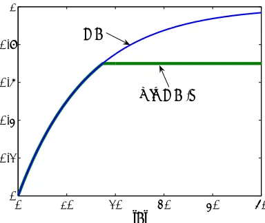
),c}, the original function Fi truncated at score level c. The key insight is that

these truncated functionsFi,cremain monotonic and submodular (Fujito, 2000). Figure 4 illustrates

this truncation concept. Let Fc(

A

) =_m1∑iFi,c(

A

) be their average value. Since monotonic

sub-modular functions are closed under convex combinations, Fc is also submodular and monotonic.

Furthermore, Fi(

A

)≥c for all 1≤i≤m if and only if Fc(

A

) =c. Hence, in order to determine

whether some c is feasible for Problem (5), we need to determine whether there exists a set of size at mostαk such that Fc(

A

) =c. Note, that due to monotonicity of Fcand the choice of c it holds

that that c=Fc(

V

). We hence need to solve the following optimization problem:

A

c∗=argmin

A⊆V

|

A

|, such that Fc(

A

) =Fc(

V

). (6)

Problems of the form min_A|

A

| such that F(

A

) =F(

V

), where F is a monotonic submodular function, are called submodular covering problems. Since Fc satisfies these requirements, the

MINCOVERcProblem (6) is an instance of such a submodular covering problem. While such

prob-lems are NP-hard in general (Feige, 1998), Wolsey (1982) shows that the greedy algorithm, that starts with the empty set (

A

=/0) and iteratively adds the element s increasing the score the most until F(

A

) =F(

V

), achieves near-optimal performance on this problem. We can hence use the greedy algorithm applied to the truncated functions Fc as our approximate algorithm GPC, which

is formalized in Algorithm 1. Using Wolsey’s result and the observation that α can be chosen

independently of the truncation threshold c, we find:

Lemma 4 Given integral valued1monotonic submodular functions F1,...,Fmand a (feasible) con-stant c, Algorithm 1 (with input Fc) finds a set

A

Gsuch that Fi(

A

G)≥c for all i, and|

A

G| ≤α|

A

c∗|, where

A

c∗is an optimal solution to Problem (6), and

α=1+log

max

s∈V

∑

i Fi({s})

.

We can compute this approximation guaranteeαfor any given instance of the RSOS problem.

Hence, if for a given value of c the greedy algorithm returns a set of size greater thanαk, there cannot

exist a solution

A

with|

A

| ≤k with Fi(

A

)≥c for all i. Thus, c is an upper bound to the RSOS

Problem (3). We can use this argument to conduct the binary search discussed in Section 4.1 to find the optimal value of c. The binary search procedure maintains an interval[cmin,cmax], initialized

[0,miniFi(

V

)]. At every iteration, we test the current center of the interval, c= (cmin+cmax)/2,

and check feasibility of c using the greedy algorithm. If c is feasible, we retain the current best feasible solution and set cmin=c. If c is infeasible (which we detect by comparing the number of

elements picked by the greedy algorithm withαk), we set cmax=c.

0 10 20 30 40 50 0

0.2 0.4 0.6 0.8 1

|A| F(A)

min(F(A),c)

Figure 4: Truncating an objective function F preserves submodularity and monotonicity.

GPC (Fc, c)

A

← /0;

while Fc(

A

)<c do

foreach s∈

V

\

A

do δs←Fc(

A

∪ {s})−Fc(

A

);

A

←

A

∪ {argmax_sδs}; end

Algorithm 1: The greedy submodular partial cover (GPC) algorithm.

We call Algorithm 2, which formalizes this procedure, the submodular saturation algorithm (SATURATE), as the algorithm considers the truncated objectivesFi,c, and chooses sets which satu-rate all these objectives. In the pseudo-code of Algorithm 2 we passαas a parameter. Theorem 5

(given below) states that SATURATE, when applied withα chosen as in Lemma 4, is guaranteed

to find a set which achieves worst-case score miniFi at least as high as the optimal solution, if we

allow the set to be logarithmically (a factorα) larger than the optimal solution.

Theorem 5 For any integer k, SATURATEfinds a solution

A

Ssuch that

min

i Fi(

A

S)≥_|max_A|≤kmini Fi(

A

) and |

A

S| ≤αk,

forα=1+log(max_s∈V∑_iFi({s})). The total number of submodular function evaluations is

O

|

V

|2_{m log}

m min i Fi(

V

)

.

Note, that the algorithm still makes sense for any value ofα. However, ifα<1+log(maxs∈V∑iFi({s})),

the guarantee of Theorem 5 does not hold. As argued in Section 4.1, if we had an exact algorithm for

submodular coverage, then we would setα=1, and SATURATEwould return the optimal solution

to the RSOS problem. Since, in our experience, the greedy algorithm for optimizing submodular functions works very effectively (cf., Krause et al. 2007b), in our experiments, we call SATURATE

SATURATE(F1,...,Fm,k,α)

cmin←0; cmax←miniFi(

V

);

A

best← /0;

while(cmax−cmin)≥_m1 do c←(cmin+cmax)/2;

Define Fc(

A

)← _m1∑imin{Fi(

A

),c};

A

←GPC(Fc,c);

if|

A

|>αk then cmax←c;

else

cmin←c;

A

best=

A

end end

Algorithm 2: The Submodular Saturation algorithm.

If we apply SATURATE to the example problem described in Section 3, we would start with

cmax=n. Running the coverage algorithm (GPC) with c=n/2 would first pick element s1(or s2),

since Fc({s1}) =n/2, and, next, pick s2(or s1resp.), hence finding the optimal solution.

The worst-case running time guarantee is quite pessimistic, and in practice the algorithm is much faster: Using a priority queue and lazy evaluations, Algorithm 1 can be sped up drastically. Lazy evaluations exploit the fact that, due to submodularity, the differencesδs(

A

) =Fc(

XA

∪s)− Fc(

XA

) that are computed by GPC are monotonically decreasing in

A

, which allows to avoid a

large number of function evaluations (cf., Robertazzi and Schwartz 1989 for details). In addition, for many submodular functions Fi, such as the variance reduction, it is often cheaper to compute Fc(

XA

∪s)−Fc(

XA

)instead of Fc(

XA

∪s). This observation can be exploited to drastically speed up

GPC. Furthermore, in practical implementations, one would stop GPC onceαk+1 elements have

been selected, which already proves that the optimal solution with k elements cannot achieve score

c. Also, Algorithm 2 can be terminated once cmax−cminis sufficiently small; in our experiments,

10-15 iterations usually sufficed.

5. Hardness of Bicriterion Approximation

Guarantees of the form presented in Theorem 5 are often called bicriterion guarantees. Instead of requiring that the obtained objective score is close to the optimal score and all constraints are exactly met, a bicriterion guarantee requires a bound on the suboptimality of the objective, as well

as bounds on how much the constraints are violated. Theorem 3 showed that—unless P=NP—no

approximation guarantees can be obtained which do not violate the constraint on the cost k, thereby necessitating the bricriterion analysis.

One might ask, whether the guarantee on the size of the set,α, can be improved. Unfortunately, this is not likely, as the following result shows:

Theorem 6 If there were a polynomial time algorithm which, for any integer k, is guaranteed to

find a solution

A

Ssuch that miniFi(

A

S)≥max_|A|≤kminiFi(

A

)and|

A

S| ≤βk, whereβ≤(1−ε)(1+

Hereby, DTIME(nlog log n)is a class of deterministic, slightly superpolynomial (but sub-exponential) algorithms (Feige, 1998); the inclusion NP⊆DTIME(nlog log n)is considered unlikely (Feige, 1998).

Taken together, Theorem 3 and Theorem 6, provide strong theoretical evidence that SATURATE

achieves best possible theoretical guarantees for the problem of maximizing the minimum over a set of submodular functions.

6. Examples of Robust Submodular Observation Selection problems

We now demonstrate that many important machine learning problems can be phrased as RSOS problems. Section 8 provides more details and experimental results for these domains.

6.1 Minimizing the Maximum Kriging Variance

Consider a Gaussian Process (GP) (cf., Rasmussen and Williams, 2006)

X

V defined over a finite set of locations (indices)

V

. Hereby,

X

V is a set of random variables, one variable

X

s for each

location s∈

V

. Given a set of locations

A

⊆

V

which we observe, we can compute the predictive distribution P(

X

V\A |

XA

=xA), that is, the distribution of the variables

X

V\A at the unobserved locations

V

\

A

, conditioned on the measurements at the selected locations,

XA

=x_A. Let σ2_s|A be the residual variance after making observations at

A

. Let Σ_AA be the covariance matrix of the measurements at the chosen locations

A

, andΣsA be the vector of cross-covariances between the measurements at s and

A

. Then, the predictive variance (often called Kriging variance in the geostatistics literature), given by

σ2

s|A=σ2s−ΣsAΣ−_AA1ΣAs,

depends only on the set

A

, and not on the observed values x_A.2 As argued in Section 2, an often (especially in the case of nonstationary phenomena) appropriate criterion is to select locations

A

such that the maximum marginal variance is as small as possible, that is, we want to select a subset

A

∗⊆

V

of locations to observe such that

A

∗=argmin

|A|≤k maxs∈V σ

2

s|A. (7)

Let us assume for now that the a priori varianceσ2_s is constant for all locations s (in Section 7, we show how our approach generalizes to non-constant marginal variances). Furthermore, let us define the variance reduction Fs(

A

) =σ2s−σ2s|A. Solving Problem (7) is then equivalent to maximizing the minimum variance reduction over all locations s. For a particular location s, Das and Kempe (2008) show that the variance reduction Fs(often) is a monotonic submodular function. Hence the

problem

A

∗=argmax

|A|≤k mins∈VFs(

A

) =argmax_|A|≤k mins∈Vσ

2 s−σ2s|A is an instance of the RSOS problem.

6.2 Variable Selection under Parameter Uncertainty

Consider an application, where we want to diagnose a failure of a complex system, by perform-ing a number of tests. We can model this problem by usperform-ing a set of discrete random variables

X

V ={

X

1,...,

X

n} indexed by

V

={1,...,n}, which model both the hidden state of the system

and the outcomes of the diagnostic tests. The interaction between these variables is modeled by a joint distribution P(

X

_V |θ) with parametersθ. Krause et al. (2007b) and Krause and Guestrin (2005) show that many variable selection problems can be formulated as the problem of optimizing a submodular utility function (measuring, for example, the information gain I(

XU

,

XA

)with respect to some variables of interest

U

, or the mutual information I(

XA

;

X

_V\A)between the observed and unobserved variables, etc.). However, the informativeness of a chosen set

A

typically depends on the particular parametersθ, and these parameters might be uncertain. In some applications, it might not be reasonable to impose a prior distribution over θ, and we may want to perform well even under the worst-case parameters. In these cases, we can associate, with each parameter settingθ, a different submodular objective function F_θ, for example,

F_θ(

A

) =I(

XA

;

XU

|θ),

and we might want to select a set

A

which simultaneously performs well for all possible parameter values. In practice, we can discretize the set of possible parameter values θ(for example around a 95% confidence interval estimated from initial data) and optimize the worst case F_θ over the resulting discrete set of parameters.

6.3 Robust Experimental Designs

Another application is experimental design under nonlinear dynamics (Flaherty et al., 2006). The goal is to estimate a set of parametersθof a nonlinear function y= f(x,θ) +w, by providing a

set of experimental stimuli x, and measuring the (noisy) response y. In many cases, experimental design for linear models (where y=A(x)Tθ+w with Gaussian noise w) can be efficiently solved

by semidefinite programming (Boyd and Vandenberghe, 2004). In the nonlinear case, a common approach (cf., Chaloner and Verdinelli, 1995) is to linearize f around an initial parameter estimate θ0, that is,

y= f(x,θ0) +V(x)(θ−θ0) +w, (8)

where V(x)is the Jacobian of f with respect to the parametersθ, evaluated atθ0. Subsequently, a locally-optimal design is sought, which is optimal for the linear design Problem (8) for initial

pa-rameter estimatesθ0. Flaherty et al. (2006) show that the efficiency of such a locally optimal design

can be very sensitive with respect to the initial parameter estimatesθ0. Consequently, they develop

an efficient semi-definite program (SDP) for E-optimal design (i.e., the goal is to minimize the max-imum eigenvalue of the error covariance) which is robust against perturbations of the Jacobian V . However, it might be more natural to directly consider robustness with respect to perturbation of the initial parameter estimatesθ0, around which the linearization is performed. We show how to find

(Bayesian A-optimal) designs which are robust against uncertainty in these parameter estimates. In this setting, the objectives F_θ0(

A

)are the reductions of the trace of the parameter covariance,

F_θ0(

A

) =tr Σ

(θ0)

θ

−tr Σ(θ0)

θ|A

7DUJHWRI

FRQWDPLQDWLRQ

6HQVRUV

6HQVRUV

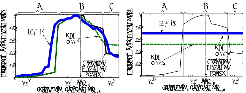
Figure 5: Securing a municipal water distribution network against contaminations performed under knowledge of the sensor placement is another instance of the RSOS problem.

whereΣ(θ0)_{is the joint covariance of observations and parameters after linearization around}θ

0; thus, F_θ0 is the sum of marginal parameter variance reductions, which are (often) individually monotonic

and submodular (Das and Kempe, 2008), and so F_θ0 is monotonic and submodular as well. Hence,

in order to find a robust design, we maximize the minimum variance reduction, where the minimum is taken over (a discretization into a finite subset of) all initial parameter valuesθ0.

6.4 Sensor Placement for Outbreak Detection

Another class of examples are outbreak detection problems on graphs, such as contamination detec-tion in water distribudetec-tion networks (Leskovec et al., 2007). Here, we are given a graph

G

= (

V

,

E

), and a phenomenon spreading dynamically over the graph. We define a set of intrusion scenarios

I

; each scenario i∈

I

models an outbreak (e.g., spreading of contamination) starting from a given node s∈

V

in the network. By placing sensors at a set of locations

A

⊆

V

, we can detect such an outbreak, and thereby minimize the adverse effects on the network.

More formally, for each possible outbreak scenario i∈

I

and for each node v∈

V

we define the detection time Ti(v)as the time when the outbreak affects node v (and Ti(v) =∞if node v is

never affected). We furthermore define a penalty functionπi(t)which models the penalty incurred

for detecting outbreak i at time t. We requireπi(t)to be monotonically non-decreasing in t (i.e., we

never prefer late over early detection), and bounded above byπi(∞)∈R. Our goal is to minimize

the worst-case penalty: We extendπi to observation sets

A

asπi(

A

) =πi(mins∈ATi(s)). Then, our

goal is to solve

A

∗=argmin

|A|≤k

max

i∈I πi(

A

).

Equivalently, we can define the penalty reduction Fi(

A

) =πi(∞)−πi(

A

). Clearly, Fi(/0) =0, Fi

is monotonic. In Leskovec et al. (2007), it was shown that Fiis also guaranteed to be submodular.

For now, let us assume thatπi(∞)is constant for all i (we will relax this assumption in Section 7.2).

reduction is as large as possible, that is, we want to select

A

∗=argmax

|A|≤k mini∈I Fi(

A

).

In other words, an adversary observes our sensor placement

A

, and then decides on an intrusion i for which our utility Fi(

A

)is as small as possible. Hence, our goal is to find a placement

A

which

performs well against such an adversarial opponent.

6.5 Robustness Against Sensor Failures and Feature Deletion

Another interesting instance of the RSOS problem arises in the context of robust sensor placements. For example, in the outbreak detection problem, sensors might fail, due to hardware problems or manipulation by an adversary. We can model this problem in the following way: Consider the case where all sensors at a subset

B

⊆

V

of locations fail. Given a submodular function F (e.g., the utility for placing a set of sensors), and the set

B

⊆

V

of failing sensors, we can define a new function F_B(

A

) =F(

A

\

B

), corresponding to the (reduced) utility of placement

A

after the sensor failures. It is easy to show that if F is nondecreasing and submodular, so is F_B. Hence, the problem of optimizing sensor placements which are robust to sensor failures results in a problem of simultaneously maximizing a collection of submodular functions, for example, for the worst-case failure of k<k sensors we solve

A

∗=argmax

|A|≤k

min

|B|≤kFB(

A

).

We can also combine the optimization against adversarial contamination scenarios as discussed in Section 6.3 with adversarial sensor failures, and optimize3

A

∗=argmax

|A|≤k

min

i∈I |Bmin|≤kFi(

A

\

B

).

Another important problem in machine learning is feature selection. In feature selection, the goal is to select a subset of features which are informative with respect to, for example, a given clas-sification task. One objective frequently considered is the problem of selecting a set of features which maximize the information gained about the class variable

X

Y after observing the features

XA

, F(

A

) =H(

X

Y)−H(

X

Y |

XA

), where H denotes the Shannon entropy. Krause and Guestrin (2005)

show, that in a large class of graphical models, the information gain F(

A

)is in fact a submodular function. Now we can consider a setting, where an adversary can delete features which we selected (as considered, for example, by Globerson and Roweis 2006). The problem of selecting features ro-bustly against such arbitrary deletion of, for example, m features, is hence equivalent to the problem of maximizing min_|B|≤mFB(

A

), where

B

are the deleted features.

6.5.1 IMPROVEDGUARANTEES FORSENSORFAILURES

As discussed above, in principle, we could find a placement robust to single sensor failures by using SATURATEto (approximately) solve

A

∗=argmax

|A|≤k

min

s Fs(

A

).

However, since |

V

| can be very large, and the approximation guarantee α depends

logarithmi-cally on |

V

|, such a direct approach might not be desirable. We can improve the guarantee from

O

(log|

V

|)to

O

(log(k log|

V

|)), which typically is much tighter, if k |

V

|/log|

V

|(i.e., we place far fewer sensors than we have possible sensor locations). We can improve the approximation guar-antee drastically by noticing that Fs(

A

) =F(

A

)if s∈/

A

. Hence,

Fc(

A

) =|

V

| − |

A

|

|

V

| min{F(

A

),c}+

1

|

V

|_s

∑

_∈AFs,c(

A

).

We can replace this objective by a new objective function,

F_c(

A

) =k− |

A

|

k min{F(

A

),c}+

1

k_s

∑

_∈AFs,c(

A

)

for some constant ˆk to be specified below. This modified objective is still monotonic and submodular when restricted to sets of size at most ˆk. It still holds that, for all subsets|

A

| ≤ˆk, that

F_c(

A

)≥c⇔Fs(

A

)≥c for all s∈

V

.

How large should we choose ˆk? We have to choose ˆk large enough such that SATURATEwill never choose sets larger than ˆk. A sufficient choice for ˆk is henceαk, whereα=1+log(|

V

|max_s∈VF({s})). For this choice of ˆk, our new approximation guarantee will be

α=1+log

αk max s∈V F({s})

=1+log

1+log

|

V

|max

s∈V F({s})

k max s∈V F({s})

≤1+2 log

k log(|

V

|)max

s∈V F({s})

Hence, for the new objective F_c, we get a tighter approximation guarantee, α = 1+

2 log(k log(|

V

|)max_s∈VF({s})), which now depends logarithmically on k log|

V

|, instead of the number of available locations|

V

|. Note that this same approach can also provide tighter approxi-mation guarantees in the case of multiple sensor failures.

7. Extensions

7.1 Non-integral Objectives

In our analysis of SATURATE(Section 4), we have assumed, that each of the objective functions Fi

only take values in the positive integers. However, most objective functions of interest in observation selection (such as those discussed in Section 6) typically do not meet this assumption. If the Fitake

on rational numbers, we can scale the objectives by multiplying by their common denominator. If we allow small additive approximation error (i.e., are indifferent if the approximate solution differs from the optimal solution in low order bits), we can also approximate the values assumed by the functions Fi by their highest order bits. In this case, we replace the functions Fi(

A

) by the

approximations

F_i(

A

) =2

j_F i(

A

)

2j .

By construction, F_i(

A

)≤Fi(

A

)≤Fi(

A

)(1+2−j), that is, Fi is within a factor of(1+2−j)of Fi.

Also, 2jF_i(

A

) is integral. However, F_i(

A

) is not guaranteed to be submodular. Nevertheless, an analysis similar to the one presented by Krause et al. (2007b) can be used to bound the effect of this approximation on the theoretical guaranteesαobtained by the algorithm, which will now scale linearly with the number j of high order bits considered. In practice, as we show in Section 8, SAT

-URATE provides state-of-the-art performance, even without rounding the objectives to the highest order bits.

7.2 Non-constant Thresholds

Consider the example of minimizing the maximum variance in Gaussian Process regression. Here, the Fi(

A

) =σ2i−σ2i|Adenote the variance reductions at location i. However, rather than guaranteeing that Fi(

A

)≥c for all i (which, in this example, means that the minimum variance reduction is c), we want to guarantee that σ2_i|A ≤c for all i, which requires a different amount of variance

reduction for each location. We can easily adapt our approach to handle this case: Instead of defining

Fi,c(

A

) =min{Fi(

A

),c}, we defineFi,c(

A

) =min{Fi(

A

),σ2i −c}, and then again perform binary

search over c, but searching for the smallest c instead. The algorithm, using objectives modified in this way, will bear the same approximation guarantees.

7.3 Non-uniform Observation Costs

We can extend SATURATE to the setting where different observations have different costs. In

the spatial monitoring setting for example, certain locations might be more expensive to acquire

a measurement from. Suppose a cost function g :

V

→R+ assigns each element s∈

V

a

posi-tive cost g(s); the cost of a set of observations is then g(

A

) =∑s∈Ag(s). The problem is to find

A

∗=argmax_A⊂VminiFi(

A

)subject to g(

A

)≤B, where B>0 is a budget we can spend on making

observations. In this case, we use the rule

δs←

Fc(

A

∪ {s})−Fc(

A

) g(s)

7.4 Handling More Complex Cost Functions

So far, we considered problems where we are given an additive cost function g(

A

)over the possible

sets

A

of observations. In some applications, more complex cost functions arise. For example,

when placing wireless sensor networks, the placements

A

should not only be informative (i.e., Fi(

A

)

should be high for all utility functions Fi), but the placement should also have low communication cost. Krause et al. (2006) describe such an approach, where the cost g(

A

)measures the expected

number of retransmissions required for sending messages across an optimal routing tree connecting

the sensors

A

. Formally, the observations s are considered to be nodes in a graph

G

= (

V

,

E

), with edge weights w(e)for each edge e∈

E

. The cost g(

A

)is the cost of a minimum Steiner Tree (cf., Vazirani 2003) connecting the observations

A

in the graph

G

.

More generally, we want to solve problems of the form

argmax A

min

i Fi(

A

)subject to g(

A

)≤B,

where g(

A

)is a complex cost function. The key insight of the SATURATEalgorithm is that the non-submodular robust optimization problem can be approximately solved by solving a non-submodular covering problem. In the case where g(

A

) =|

A

|this problem requires solving (6). More generally,

we can apply SATURATEto any problem where we can (approximately) solve

A

c=argmin

A⊆V

g(

A

), such that Fc(

A

) =c. (9)

Problem (9) can be (approximately) solved for a variety of cost functions, such as those arising from communication constraints (Krause et al., 2006) and path constraints (Singh et al., 2007; Meliou et al., 2007).

Let us summarize our analysis as follows:

Proposition 7 Assume we have an algorithm which, given a monotonic submodular function F and

a cost function g, returns a solution

A

such that F(

_A

) =F(

_V

)and

g(

A

)≤αF min

A:F(A)=F(V)g(

A

),

where αF depends on the function F. SATURATE, using this covering algorithm, can obtain a solution

A

Sto the RSOS problem such that

min

i Fi(

A

S)≥gmax(A)≤Bmini Fi(

A

), and

g(

A

S)≤αFB,

whereα_F is the approximation factor of the covering algorithm, when applied to F= _m1∑iFi.

Note that the formalism developed in this section also allows to handle robust versions of com-binatorial optimization problems such as the Knapsack (cf., Martello and Toth, 1990), Orienteering (cf., Laporte and Martello, 1990; Blum et al., 2003) and Budgeted Steiner Tree (cf., Johnson et al., 2000) problems. In these problems, instead of a general submodular objective function, the special case of a modular (additive) function F is optimized:

A

∗=argmax

0 50 100 150 200 250 300 350 0

1000 2000 3000 4000 5000 6000 7000

Average−case population affected

Worst

−

case population affected

Knee in Pareto curve Only optimize for

average case

Only optimize for worst case

Figure 6: Tradeoff curve for simultaneously optimizing the average- and worst-case score in the water distribution network monitoring application. Notice the knee in the tradeoff curve, indicating that by performing multi-criterion optimization, solutions performing well for both average- and worst-case scores can be obtained.

The problems differ only in the choice of the complex cost function. In Knapsack for example, g is additive, in the Budgeted Steiner Tree problem, g(

A

)is the cost of a minimum Steiner tree con-necting the nodes

A

in a graph, and in Orienteering, g(

A

)is the cost of a shortest path connecting the nodes

A

in a graph. In practice, often the utility function F(

A

) is not exactly known, and a solution is desired which is robust against worst-case choice of the utility function. Since modular functions are a special case of submodular functions, such problems can be approximately solved using Proposition 7.

7.5 Trading Off Average-case and Worst-case Scores

In some applications, optimizing the worst-case score Fwc(

A

) =miniFi(

A

) might be a too

pes-simistic approach. On the other hand, ignoring the worst-case and only optimizing the average-case (the expected score under a distribution over the objectives) Fac(

A

) = _m1∑iFi(

A

)might be too

op-timistic. In fact, in Section 8 we show that optimizing the average-case score Faccan often lead to

drastically poor worst-case scores. In general, we might be interested in solutions, which perform well both in the average- and worst-case scores.

Formally, we can define a multicriterion optimization problem, where we intend to optimize the vector [Fac(

A

),Fwc(

A

)]. In this setting, we can only hope for Pareto-optimal solutions (cf.,

Boyd and Vandenberghe, 2004, in the context of convex functions). A set

A

∗, |

A

∗| ≤k is called Pareto-optimal, if it is not dominated, that is, there does not exist another set

B

, |

B

| ≤k with Fac(

B

)>Fac(

A

∗)and Fwc(

B

)≥Fwc(

A

∗)(or Fac(

B

)≥Fac(

A

∗)and Fwc(

B

)>Fwc(

A

∗)).

One possible approach to find such Pareto-optimal solutions is constrained optimization:4 for a specified value of cac, we desire a solution to

A

∗=argmax

|A|≤k

Fwc(

A

)such that Fac(

A

)≥cac. (10)

By specifying different values of cacin (10), we would obtain different Pareto-optimal solutions.5

Figure 6 presents an example of several Pareto-optimal solutions, based on data from the outbreak detection problem (Details will be discussed in Section 8.3). This curve shows that, using the techniques described below, multicriterion solutions can be found which combine the advantages of worst-case and average-case solutions.

We can modify SATURATEto solve Problem (10) in the following way. Let us again assume

we know the optimal value cwc achievable for Problem (10). Then, Problem (10) is equivalent to

solving

A

∗=argmin

A |

A

|

subject to Fwc(

A

)≥cwcand Fac(

A

)≥cac.

Now, using our notation from Section 4, this problem is again equivalent to

A

∗=argmin

A |

A

|

subject to Fcwc,cac =cwc+cac, (11)

where

Fcwc,cac(

A

) =Fcwc(

A

) +min{Fac(

A

),cac}.

Note that Fcwc,cac is a submodular function, and hence (11) is a submodular covering problem, which

can be approximately solved using the greedy algorithm.

For any choice of cac, we can find the optimal value of cwcby performing binary search on cwc.

We summarize our analysis in the following Theorem:

Theorem 8 For any integer k and constraint cac, SATURATE finds a solution

A

S (if it exists) such that

Fwc(

A

S)≥ max |A|≤k,Fac(A)≥cac

Fwc(

A

),

Fac(

A

S)≥cac, and |

A

S| ≤αk, for α=1+log(2 maxs∈V∑iFi({s})). Each such solution

A

S is

approximately Pareto-optimal, that is, there does not exist a set

B

,|

B

| ≤k such that

B

dominates

A

S. The total number of submodular function evaluations is

O

|

V

|2_{m log(∑}

iFi(

V

))

.

8. Experimental Results

In this section, we present experimental results on several robust observation selection problems.

8.1 Minimizing the Maximum Kriging Variance

0 20 40 60 80 100 0.5 1 1.5 2 2.5

Number of sensors

Maximum marginal variance

Greedy Saturate Simulated Annealing (SA) Saturate + SA

(a) [P] Algorithm comparison

0 5 10 15 20

0 0.5 1 1.5 2 2.5 3

Number of sensors

Marginal variance

Max. var. opt. avg.

(Greedy) Max. var. opt. max. (Saturate) Avg. var. opt. max. (Saturate) Avg. var. opt. avg. (Greedy)

(b) [P] Avg. vs max. variance

0 10 20 30 40

10−1 100

Number of sensors

Maximum marginal variance

Greedy Saturate

Saturate + SA

SA

(c) [T] Algorithm comparison

2 4 6 8 10

10−2 10−1 100

Number of sensors

Marginal variance

Max. var. opt. avg.

(Greedy) _{opt. max.}Max. var. (Saturate) Avg. var.

opt. max. (Saturate)

Avg. var. opt. avg. (Greedy)

(d) [T] Avg. vs max. variance

0 20 40 60

0 0.05 0.1 0.15 0.2 0.25

Number of sensors

Maximum marginal variance

Greedy

Simulated

annealing Saturate + SA

Saturate

(e) [L] Algorithm comparison

0 5 10 15 20

0 0.05 0.1 0.15 0.2 0.25

Number of sensors

Marginal variance

Max. var. opt. avg.

(Greedy) Max. var. opt. var. (Saturate) Avg. var. opt. max. (Saturate) Avg. var. opt. avg. (Greedy)

(f) [L] Avg. vs max. variance

Figure 7: (a,c,e) SATURATE, greedy and SA on the (a) precipitation, (b) building temperature and

(c) lake temperature data. SATURATE performs comparably with the fine-tuned SA

0 10 20 30 40 50 60 0

100 200 300 400 500

Number of observations

Running time (s)

Simulated Annealing (SA)

Saturate+SA Saturate

Greedy

Figure 8: Running time for algorithms on the precipitation data set [P].

In the geostatistics literature, the predominant choice of optimization algorithms for selecting locations in a GP to minimize the (maximum and average) predictive variance are carefully tuned lo-cal search procedures, prominently simulated annealing (cf., Sacks and Schiller 1988; Wiens 2005;

van Groenigen and Stein 1998). We compare our SATURATEalgorithm against a state-of-the-art

implementation of such a simulated annealing (SA) algorithm, first proposed by Sacks and Schiller (1988). We use an optimized implementation described recently by Wiens (2005). This algorithm has 7 parameters which need to be tuned, describing the annealing schedule, distribution of itera-tions among several inner loops, etc. We use the parameter settings as reported by Wiens (2005), and present the best result of the algorithm among 10 random trials. In order to compare observation sets of the same size, we called SATURATEwithα=1.

Figures 7(a), 7(c) and 7(e) compare simulated annealing, SATURATE, and the greedy algorithm which greedily selects elements which decrease the maximum variance the most on the three data sets. We also used SATURATEto initialize the simulated annealing algorithm (using only a single run of simulated annealing, as opposed to 10 random trials). In all three data sets, SATURATE ob-tains placements which are drastically better than the placements obtained by the greedy algorithm. Furthermore, the performance is very close to the performance of the simulated annealing algo-rithm. In our largest monitoring data set [P], SATURATE even strictly outperforms the simulated annealing algorithm when selecting 30 and more sensors. Furthermore, as Figure 8 shows, SATU

-RATEis significantly faster than simulated annealing, by factors of 5-10 for larger problems. When using SATURATEin order to initialize the simulated annealing algorithm, the resulting performance almost always resulted in the best solutions we were able to find with any method, while still exe-cuting faster than simulated annealing with 10 random restarts as proposed by Wiens (2005). These results indicate that SATURATEcompares favorably to state-of-the-art local search heuristics, while being faster, requiring no parameters to tune, and providing theoretical approximation guarantees.

Optimizing for the maximum variance could potentially be considered too pessimistic. Hence

we compared placements obtained by SATURATE, minimizing the maximum marginal posterior

variance, with placements obtained by the greedy algorithm, where we minimize the average marginal variance. Note, that, whereas the maximum variance reduction is non-submodular, the average vari-ance reduction is (often) submodular (Das and Kempe, 2008), and hence the greedy algorithm can

be expected to provide near-optimal placements. Figures 7(b), 7(d) and 7(f) present the maximum and average marginal variances for both algorithms. On all three data sets, our results show that if we optimize for the maximum variance we still achieve comparable average variance. If we optimize for average variance however, the maximum posterior variance remains much higher.

8.2 Robust Experimental Design

We consider the robust design of experiments (cf., Section 6.3) for the Michaelis-Menten mass-action kinetics model, as discussed by Flaherty et al. (2006). The goal is least-square parameter estimation for a function y= f(x,θ), where x is the chosen experimental stimulus (the initial

sub-strate concentration S0), andθ= (θ1,θ2)are two parameters as described by Flaherty et al. (2006).

The stimulus x is chosen from a menu of six options, x∈ {1/8,1,2,4,8,16}, each of which can be repeatedly chosen. The goal is to produce a fractional design w= (w1,...,w6), where each

com-ponent wimeasures the relative frequency according to which the stimulus xiis chosen. Since f is

nonlinear, f is linearized around an initial parameter estimateθ0= (θ01,θ02), and approximated by

its Jacobian V_θ0. Classical experimental design considers the error covariance of the least squares

estimate ˆθ, Cov(θˆ|θ0,w) =σ2(V_θT₀WVθ0)−

1_{, where W =diag(w), and aims to find designs w which}

minimize this error covariance. E-optimality, the criterion adopted by Flaherty et al. (2006), mea-sures smallness in terms of the maximum eigenvalue of the error covariance matrix. The optimal w can be found using Semidefinite Programming (SDP) (Boyd and Vandenberghe, 2004).

The estimate Cov(_θˆ _{|θ0,w) depends on the initial parameter estimateθ0, where linearization} is performed. However, since the goal is parameter estimation, a “certain circularity is involved” (Flaherty et al., 2006). To avoid this problem, Flaherty et al. (2006) find a design w_ρ(θ0)by solving

a robust SDP which minimizes the error size, subject to a worst-case perturbationΔon the Jacobian

V_θ0; the robustness parameterρ bounds the spectral norm ofΔ. As evaluation criterion, Flaherty

et al. (2006) define a notion of efficiency, which is the error size of the optimal design with correct initial parameter estimate, divided by the error when using a robust design obtained at the wrong initial parameter estimates, that is,

efficiency≡λmax[Cov(θˆ |θtrue,wopt(θtrue)))] λmax[Cov(θˆ |θtrue,wρ(θ0))]

,

where wopt(θ) is the E-optimal design for parameterθ. They show that for appropriately chosen

values ofρ, the robust design is more efficient than the optimal design, if the initial parameterθ0

does not equal the true parameter.

While their results are very promising, an arguably more natural approach than perturbing the Jacobian would be to perturb the initial parameter estimate, around which linearization is performed. For example, if the function f describes a process which behaves characteristically differently in different “phases”, and the parameterθcontrols which of the phases the process is in, then a robust design should intuitively “hedge” the design against the behavior in each possible phase. In such a case, the uniform distribution (which the robust SDP chooses for largeρ) would not be the most robust design.

A B C

10-1 100 101

0 0.2 0.4 0.6 0.8 1

Initial parameter estimate θ₀₂

Effi cie n cy (w .r .t . E-op tim a lit y ) Classical E-optimal design SDP

ρ= 10-3

true θ₂

Saturate

10-1 100 101

0 0.2 0.4 0.6 0.8 1

Initial parameter estimate θ₀₂

Effi cie n cy (w .r .t . E-op tim a lit y ) Classical E-optimal design SDP

ρ= 10-3

true θ₂

Saturate

(a) Low uncertainty inθ0

A B C

10-1 100 101

0 0.2 0.4 0.6 0.8 1

Initial parameter estimate θ

02 Effi cie n cy (w .r .t . E-op tim a lit y ) Classical E-optimal design SDP

ρ= 10-3

true θ

2 Saturate

SDP

ρ= 16.3

10-1 100 101

0 0.2 0.4 0.6 0.8 1

Initial parameter estimate θ

02 Effi cie n cy (w .r .t . E-op tim a lit y ) Classical E-optimal design SDP

ρ= 10-3

true θ

2 Saturate

SDP

ρ= 16.3

(b) High uncertainty inθ0

Figure 9: Efficiency of robust SDP of Flaherty et al. (2006) and SATURATEon a biological experi-mental design problem. (a) Low assumed uncertainty in initial parameter estimates: SDP performs better in region C, SATURATE performs better in region A. (b) High assumed uncertainty in initial parameter estimates: SATURATEoutperforms the SDP solutions.

eigenvalue size of the covariance matrix. Furthermore, we equip the parametersθwith an uninfor-mative normal prior (which we chose as diag([202_,202_{])) as typically done in Bayesian experimental}

design. We then minimize the expected trace of the posterior error covariance, tr(Σ_θ|A). Hereby,

A

is a discrete design of 20 experiments, where each option xican be chosen repeatedly. In order to

apply SATURATE, for eachθ0, we define Fθ0(

A

)as the normalized variance reduction

F_θ0(

A

) = 1

Z_θ0

tr Σ(θ0)

θ

−tr Σ(θ0)

θ|A

.

The normalization Z_θ0 is chosen such that Fθ0(

A

) =1 if

A

=argmax

|A_|=20 Fθ0(

A

_),

that is, if

A

is chosen to maximize only F_θ0. SATURATE is then used to maximize the worst-case

normalized variance reduction.

We reproduced the experiment of Flaherty et al. (2006), where the initial estimate of the second componentθ02ofθ0 was varied between 0 and 16, the “true” value beingθ2=2. For each initial

estimate ofθ02, we computed a robust design, using the SDP approach and using SATURATE, and

compared them using the efficiency metric of Flaherty et al. (2006). Note that this efficiency metric is defined with respect to E-optimality, even though we optimize Bayesian A-optimality, hence po-tentially putting SATURATEat a disadvantage. We first optimized designs which are robust against a small perturbation of the initial parameter estimate. For the SDP, we chose a robustness parameter ρ=10−3, as reported in Flaherty et al. (2006). For SATURATE, we considered an interval around [θ 1

1+ε,θ(1+ε)], discretized in a 5×5 grid, withε=.1.