Similarity-based Classification: Concepts and Algorithms

Similarity-based Classification: Concepts and Algorithms

Yihua Chen [email protected]

Eric K. Garcia [email protected]

Maya R. Gupta [email protected]

Department of Electrical Engineering University of Washington

Seattle, WA 98195, USA

Ali Rahimi [email protected]

1100 NE 45th Street Intel Research

Seattle, WA 98105, USA

Luca Cazzanti [email protected]

Applied Physics Lab University of Washington Seattle, WA 98105, USA

Editor: Alexander J. Smola

Abstract

This paper reviews and extends the field of similarity-based classification, presenting new analy-ses, algorithms, data sets, and a comprehensive set of experimental results for a rich collection of classification problems. Specifically, the generalizability of using similarities as features is ana-lyzed, design goals and methods for weighting nearest-neighbors for similarity-based learning are proposed, and different methods for consistently converting similarities into kernels are compared. Experiments on eight real data sets compare eight approaches and their variants to similarity-based learning.

Keywords: similarity, dissimilarity, similarity-based learning, indefinite kernels

1. Introduction

Similarity-based classifiers estimate the class label of a test sample based on the similarities between the test sample and a set of labeled training samples, and the pairwise similarities between the training samples. Like others, we use the term similarity-based classification whether the pairwise relationship is a similarity or dissimilarity. Similarity-based classification does not require direct access to the features of the samples, and thus the sample space can be any set, not necessarily a

Euclidean space, as long as the similarity function is well defined for any pair of samples. LetΩ

be the sample space and

G

be the finite set of class labels. Letψ:Ω_×Ω_→Rbe the similarity

function. We assume that the pairwise similarities between n training samples are given as an n_×n

similarity matrix S whose(i,j)-entry isψ(xi,xj), where xi∈Ω, i=1, . . . ,n, denotes the ith training

sample, and yi∈

G

, i=1, . . . ,n the corresponding ith class label. The problem is to estimate the

class label ˆy for a test sample x based on its similarities to the training samplesψ(x,xi), i=1, . . . ,n

Similarity-based classification is useful for problems in computer vision, bioinformatics, infor-mation retrieval, natural language processing, and a broad range of other fields. Similarity functions may be asymmetric and fail to satisfy the other mathematical properties required for metrics or inner products (Santini and Jain, 1999). Some simple example similarity functions are: travel time from one place to another, compressibility of one random process given a code built for another, and the minimum number of steps to convert one sequence into another (edit distance). Computer vision researchers use many similarities, such as the tangent distance (Duda et al., 2001), earth mover’s distance (EMD) (Rubner et al., 2000), shape matching distance (Belongie et al., 2002), and pyramid match kernel (Grauman and Darrell, 2007) to measure the similarity or dissimilarity between im-ages in order to do image retrieval and object recognition. In bioinformatics, the Smith-Waterman algorithm (Smith and Waterman, 1981), the FASTA algorithm (Lipman and Pearson, 1985) and the BLAST algorithm (Altschul et al., 1990) are popular methods to compute the similarity be-tween different amino acid sequences for protein classification. The cosine similarity bebe-tween term frequency-inverse document frequency (tf-idf) vectors is widely used in information retrieval and text mining for document classification.

Notions of similarity appear to play a fundamental role in human learning, and thus psycholo-gists have done extensive research to model human similarity judgement. Tversky’s contrast model and ratio model (Tversky, 1977) represent an important class of similarity functions. In these two models, each sample is represented by a set of features, and the similarity function is an increasing function of set overlap but a decreasing function of set differences. Tversky’s set-theoretic similar-ity models have been successful in explaining human judgement in various similarsimilar-ity assessment tasks, and are consistent with the observations made by psychologists that metrics do not account for cognitive judgement of similarity in complex situations (Tversky, 1977; Tversky and Gati, 1982; Gati and Tversky, 1984). Therefore, similarity-based classification may be useful for imitating or understanding how humans categorize.

The main contributions of this paper are: (1) we distill and analyze concepts and issues specific to similarity-based learning, including the generalizability of using similarities as features, (2) we propose similarity-based nearest-neighbor design goals and methods, and (3) we present a compre-hensive set of experimental results for eight similarity-based learning problems and eight different similarity-based classification approaches and their variants. First, we discuss the idea of similari-ties as inner products in Section 2, then the concept of treating similarisimilari-ties as features in Section 3. The generalizability of using similarities as features and that of using similarities as kernels are compared in Section 4. In Section 5, we propose design goals and solutions for similarity-based weighted nearest-neighbor learning. Generative similarity-based classifiers are discussed in Sec-tion 6. Then in SecSec-tion 7 we describe eight similarity-based classificaSec-tion problems, detail our experimental setup, and discuss the results. The paper concludes with some open questions in Sec-tion 8. For the reader’s reference, key notaSec-tion is summarized in Table 1.

2. Similarities as Inner Products

Ω sample space S n×n matrix with(i,j)-entryψ(xi,xj) G set of class labels si n×1 vector with jth elementψ(xi,xj) n number of training samples s n_×1 vector with jth elementψ(x,xj) xi∈Ω ith training sample 1 column vector of 1’s

x∈Ω test sample I identity matrix

yi∈G class label of ith training sample I_{·} indicator function y∈Gn _{n×1 vector with ith element y}

i K kernel matrix or kernel function

ˆ

y_∈G estimated class label for x k neighborhood size

D n training sample pairs{(xi,yi)}ni=1 L hinge loss function

ψ:Ω×Ω→R similarity function diag(a) diagonal matrix with a as the diagonal

Table 1: Key Notation

apply kernel classifiers. We discuss different methods for modifying similarities into kernels in Section 2.1. An important technicality is how to handle test samples, which is addressed in Sec-tion 2.2.

2.1 Modify Similarities into Kernels

The power of kernel methods lies in the implicit use of a reproducing kernel Hilbert space (RKHS) induced by a positive semidefinite (PSD) kernel (Sch¨olkopf and Smola, 2002). Although the mathe-matical meaning of a kernel is the inner product in some Hilbert space, a standard interpretation of a kernel is the pairwise similarity between different samples. Conversely, many researchers have sug-gested treating similarities as kernels, and applying any classification algorithm that only depends on inner products. Using similarities as kernels eliminates the need to explicitly embed the samples in a Euclidean space.

Here we focus on the support vector machine (SVM), which is a well-known representative of kernel methods, and thus appears to be a natural approach to similarity-based learning. All the SVM algorithms that we discuss in this paper are for binary classification1 such that yi∈ {±1}. Let y be

the n_×1 vector whose ith element is yi. The SVM dual problem can be written as

maximize

α 1

T_α

−1₂αTdiag(y)K diag(y)α

subject to 0αC1, yTα=0,

(1)

with variableα_∈Rn_{, where C>0 is the hyperparameter, K is a PSD kernel matrix whose(i,j)-entry}

is K(xi,xj), 1 is the column vector with all entries one, anddenotes component-wise inequality

for vectors. The corresponding decision function is Sch¨olkopf and Smola (2002)

ˆ

y=sgn

n

∑

i=1

αiyiK(x,xi) +b

! ,

where

b=yi− n

∑

j=1

αjyjK(xi,xj)

for any i that satisfies 0<αi <C. The theory of RKHS requires the kernel to satisfy Mercer’s

condition, and thus the corresponding kernel matrix K must be PSD. However, many similarity

functions do not satisfy the properties of an inner product, and thus the similarity matrix S can be indefinite. In the following subsections we discuss several methods to modify similarities into kernels; a previous review can be found in Wu et al. (2005). Unless mentioned otherwise, in the

following subsections we assume that S is symmetric. If not, we use its symmetric part 1₂ S+ST

instead. Notice that the symmetrization does not affect the SVM objective function in (1) since αT 1

2 S+S

T_α=1 2α

T_Sα+1 2α

T_ST_α=αT_Sα.

2.1.1 INDEFINITEKERNELS

One approach is to simply replace K with S, and ignore the fact that S is indefinite. For example, although the SVM problem given by (1) is no longer convex when S is indefinite, Lin and Lin (2003) show that the sequential minimal optimization (SMO) (Platt, 1998) algorithm will still converge with a simple modification to the original algorithm, but the solution is a stationary point instead of a global minimum. Ong et al. (2004) interpret this as finding the stationary point in a reproducing kernel Kre˘ın space (RKKS), while Haasdonk (2005) shows that this is equivalent to minimizing the

distance between reduced convex hulls in a pseudo-Euclidean space. A Kre˘ın space, denoted by

K

,

is defined to be the direct sum of two disjoint Hilbert spaces, denoted by

H

+ and

H

−, respectively.

So for any a,b_∈

K

=

H

+⊕

H

−, there are unique a+,b+∈

H

+ and unique a−,b−∈

H

− such that

a=a++a−and b=b++b−. The “inner product” on

K

is defined as

ha,b_iK =ha+,b+iH+− ha−,b−iH−,

which no longer has the property of positive definiteness. Pseudo-Euclidean space is a special case

of Kre˘ın space where

H

+and

H

−are two Euclidean spaces. Ong et al. (2004) provide a representer

theorem for RKKS that poses learning in RKKS as a problem of finding a stationary point of the risk functional, in contrast to minimizing a risk functional in RKHS. Using indefinite kernels in empirical risk minimization (ERM) methods such as SVM can lead to a saddle point solution and thus does not ensure minimizing the risk functional, so this approach does not guarantee learning in the sense of a good function approximation. Also, the nonconvexity of the problem may require intensive computation.

2.1.2 SPECTRUMCLIP

Since S is assumed to be symmetric, it has an eigenvalue decomposition S=UTΛU , where U is

an orthogonal matrix andΛis a diagonal matrix of real eigenvalues, that is, Λ=diag(λ1, . . . ,λn).

Spectrum clip makes S PSD by clipping all the negative eigenvalues to zero. Some researchers assume that the negative eigenvalues of the similarity matrix are caused by noise and view spectrum clip as a denoising step (Wu et al., 2005). Let

Λclip=diag(max(λ1,0), . . . ,max(λn,0)),

and the modified PSD similarity matrix be Sclip=UTΛclipU . Let uidenote the ith column vector of

U . Using Sclipas a kernel matrix for training the SVM is equivalent to implicitly using xi=Λ1clip/2ui

as the representation of the ith training sample since_hxi,xjiis equal to the(i,j)-entry of Sclip. A

mathematical justification for spectrum clip is that Sclipis the nearest PSD matrix to S in terms of

the Frobenius norm (Higham, 1988), that is,

Sclip=arg min

wheredenotes the generalized inequality with respect to the PSD cone.

Recently, Luss and d’Aspremont (2007) have proposed a robust extension of SVM for indefinite

kernels. Instead of only considering the nearest PSD matrix Sclip, they consider all the PSD matrices

within distanceβto S, that is,_{K0_{| k}K₋S_kF ≤β}, whereβ>minK0kK−SkF, and propose

to maximize the worst case of the SVM dual objective among these matrices:

maximize

α K0,kminK−SkF≤β

1Tα−1

2α

T_{diag(y)K diag(y)α}

subject to 0αC1, yTα=0.

This model is more flexible in the sense that the set of possible K in the hypothesis space lies in a

ball with radiusβcentered around S. Different draws of training samples will change the candidate

set of K and could cause overfitting. In practice, they replace the hard constraintkK−SkF≤βwith

a penalty term and propose the following problem as the robust SVM for S:

maximize

α minK0

1Tα₋1

2α

T_{diag(y)K diag(y)α+ρkK−Sk}2

F

subject to 0αC1, yTα=0,

(2)

whereρ>0 is the parameter to control the trade-off. They point out that the inner problem of (2) has a closed-form solution, and the outer problem is convex since its objective is a pointwise minimum

of a set of concave quadratic functions ofαand thus concave. A fast algorithm to solve (2) is given

by Chen and Ye (2008).

2.1.3 SPECTRUMFLIP

In contrast to the interpretation that negative eigenvalues are caused by noise, Laub and M¨uller (2004) and Laub et al. (2006) show that the negative eigenvalues of some similarity data can code useful information about object features or categories, which agrees with some fundamental psy-chological studies (Tversky and Gati, 1982; Gati and Tversky, 1982). In order to use the negative eigenvalues, Graepel et al. (1998) propose an SVM in pseudo-Euclidean space, and Pekalska et al. (2001) also consider a generalized nearest mean classifier and Fisher linear discriminant classifier in the same space. Following the notation in Section 2.1.1, they assume that the samples lie in a Kre˘ın space

K

=

H

+⊕

H

− with similarities given byψ(a,b) =ha+,b+iH+− ha−,b−iH−. These

proposed classifiers are their standard versions in the Hilbert space

H

=

H

+⊕

H

−with associated

inner product_ha,b_iH =_ha+,b+iH++ha−,b−iH−. This is equivalent to flipping the sign of the

neg-ative eigenvalues of the similarity matrix S: letΛflip=diag(|λ1|, . . . ,|λn|), and then the similarity

matrix after spectrum flip is Sflip=UTΛflipU . Wu et al. (2005) note that this is the same as replacing the original eigenvalues of S with its singular values.

2.1.4 SPECTRUMSHIFT

Spectrum shift is another popular approach to modifying a similarity matrix into a kernel matrix: since S+λI=UT(Λ+λI)U , any indefinite similarity matrix can be made PSD by shifting its

spec-trum by the absolute value of its minimum eigenvalue_|λmin(S)|. LetΛshift=Λ+|min(λmin(S),0)|I,

which is used to form the modified similarity matrix Sshift=UTΛshiftU . Compared with spectrum

does not change the similarity between any two different samples. Roth et al. (2003) propose

spec-trum shift for clustering nonmetric proximity data and show that Sshiftpreserves the group structure

of the original data represented by S. Let

X

be the set of samples to cluster, and _{

X

ℓ}N_ℓ=1 be a

partition of

X

into N sets. Specifically, they consider minimizing the clustering cost function2

f {

X

ℓ}Nℓ=1

=₋ N

∑

ℓ=1i,

∑

j∈Xℓ

i6=j

ψ(xi,xj) |

X

ℓ|

, (3)

where_|

X

ℓ|denotes the cardinality of set

X

ℓ. It is easy to see that (3) is invariant under spectrum

shift.

Recently, Zhang et al. (2006) proposed training an SVM only on the k-nearest neighbors of each test sample, called SVM-KNN. They used spectrum shift to produce a kernel from the similarity data. Their experimental results on image classification demonstrated that SVM-KNN performs comparably to a standard SVM classifier, but with significant reduction in training time.

2.1.5 SPECTRUMSQUARE

The fact that SST 0 for any S_∈Rn×n led us to consider using SST as a kernel, which is valid

even when S is not symmetric. For symmetric S, this is equivalent to squaring its spectrum since

SST=UTΛ2U . It is also true that using SST is the same as defining a new similarity function ˜ψfor any a,b_∈Ωas

˜

ψ(a,b) = n

∑

i=1

ψ(a,xi)ψ(xi,b).

We note that for symmetric S, treating SST as a kernel matrix K is equivalent to representing each

xi by its similarity feature vector si=

ψ(xi,x1) . . . ψ(xi,xn)

T

since Ki j =hsi,sji. The concept

of treating similarities as features is discussed in more detail in Section 3.

2.2 Consistent Treatment of Training and Test Samples

Consider a test sample x that is the same as a training sample xi. Then if one uses an ERM

clas-sifier trained with modified similarities ˜S, but uses the unmodified test similarities, represented by

vector s=ψ(x,x1) . . . ψ(x,xn)

T

, the same sample will be treated inconsistently. In general, one would like to modify the training and test similarities in a consistent fashion, that is, to modify the underlying similarity function rather than only modifying the S. In this context, given S and

˜

S, we term a transformation T on test samples consistent if T(si) is equal to the ith row of ˜S for i=1, . . . ,n.

One solution is to modify the training and test samples all at once. However, when test samples are not known beforehand, this may not be possible. For such cases, Wu et al. (2005) proposed to

first modify S and train the classifier using the modified n_×n similarity matrix ˜S, and then for each

test sample modify its s in an effort to be consistent with the modified similarities used to train the

model. Their approach is to re-compute the same modification on the augmented(n+1)_×(n+1)

similarity matrix

S′=

S s

sT ψ(x,x)

to form ˜S′, and then let the modified test similarities ˜s be the first n elements of the last column of

˜

S′. The classifier that was trained on ˜S is then applied on ˜s. To implement this approach, Wu et al.

(2005) propose a fast algorithm to perform eigenvalue decomposition of S′ by using the results of

the eigenvalue decomposition of S. However, this approach does not guarantee consistency. To attain consistency, we note that both the spectrum clip and flip modifications can be

rep-resented by linear transformations, that is, ˜S=PS, where P is the corresponding transformation

matrix, and we propose to apply the same linear transformation P on s such that ˜s=Ps. For

spec-trum flip, the linear transformation is Pflip=UTMflipU , where

Mflip=diag(sgn(λ1), . . . ,sgn(λn)).

For spectrum clip, the linear transformation is Pclip=UTMclipU , where

Mclip=diag I_{λ1≥0}, . . . ,I{λn≥0}

,

and I_{·}is the indicator function. Recall that using ˜S implies embedding the training samples in a

Euclidean space. For spectrum clip, this linear transformation is equivalent to embedding the test sample as a feature vector into the same Euclidean space of the embedded training samples:

Proposition 1 Let Sclipbe the Gram matrix of the column vectors of X∈Rm×n, where rank(X) =m.

For a given s, let x=arg minz∈RmkXTz−sk₂, then XTx=P_clips. The proof is in the appendix.

Proposition 1 states that if the n training samples are embedded in Rmwith Sclip as the Gram

matrix, and we embed the test sample in Rm by finding the feature vector whose inner products

with the embedded training samples are closest to the given s, then the inner products between the

embedded test sample and the embedded training samples are indeed ˜s=Pclips.

On the other hand, there is no linear transformation to ensure consistency for spectrum shift. For our experiments using spectrum shift, we adopt the approach of Wu et al. (2005), which for this case is to let ˜s=s, because spectrum shift only affects self-similarities.

3. Similarities as Features

Similarity-based classification problems can be formulated into standard learning problems in Eu-clidean space by treating the similarities between a sample x and the n training samples as features (Graepel et al., 1998, 1999; Pekalska et al., 2001; Pekalska and Duin, 2002; Liao and Noble, 2003). That is, represent sample x by the similarity feature vector s. As detailed in Section 4, the gener-alizability analysis yields different results for using similarities as features and using similarities as inner products.

Graepel et al. (1998) consider applying a linear SVM on similarity feature vectors by solving the following problem:

minimize

w,b

1 2kwk

2 2+C

n

∑

i=1

L(wTsi+b,yi) (4)

with variables w_∈Rn_{, b∈Rand hyperparameter C>0, where L(}α_,β_),max(1−αβ_{,0) is the}

In order to make the solution w sparser, which helps ease the computation of the discriminant function f(s) =wTs+b, Graepel et al. (1999) substitute theℓ1-norm regularization for the squared

ℓ2-norm regularization in (4), and propose a linear programming (LP) machine:

minimize

w,b kwk1+C n

∑

i=1

L(wTsi+b,yi). (5)

Balcan et al. (2008a) provide a theoretical analysis for using similarities as features, and show that if a similarity is good in the sense that the expected intraclass similarity is sufficiently large compared to the expected interclass similarity, then given n training samples, there exists a linear separator on the similarities as features that has a specifiable maximum error at a margin that de-pends on n. Specifically, Theorem 4 in Balcan et al. (2008a) gives a sufficient condition on the

similarity functionψfor (4) to achieve good generalization. Their latest results forℓ1-margin

(in-versely proportional to_kw_k1) provide similar theoretical guarantees for (5) (Balcan et al., 2008b,

Theorem 11). Wang et al. (2007) show that under slightly less restrictive assumptions on the simi-larity function there exists with high probability a convex combination of simple classifiers on the similarities as features which has a maximum specifiable error.

Another approach is the potential support vector machine (P-SVM) (Hochreiter and Obermayer, 2006; Knebel et al., 2008), which solves

minimize

α

1

2ky−Sαk 2

2+εkαk1

subject to kαk∞≤C,

(6)

where C>0 andε>0 are two hyperparameters. We note that by strong duality (6) is equivalent to

minimize

α

1

2ky−Sαk 2

2+εkαk1+γkαk∞ (7)

for someγ>0. One can see from (7) that P-SVM is equivalent to the lasso regression (Tibshirani,

1996) with an extra ℓ∞-norm regularization term. The use of multiple regularization terms in

P-SVM is similar to the elastic net (Zou and Hastie, 2005), which usesℓ1and squaredℓ2regularization

together.

The algorithms above minimize the empirical risk with regularization. In addition, Pekalska et al. consider generative classifiers for similarity feature vectors; they propose a regularized Fisher linear discriminant classifier (Pekalska et al., 2001) and a regularized quadratic discriminant classi-fier (Pekalska and Duin, 2002).

We note that treating similarities as features may not capture discriminative information if there is a large intraclass variance compared to the interclass variance, even if the classes are well-separated. A simple example is if the two classes are generated by Gaussian distributions with highly-ellipsoidal covariances, and the similarity function is taken to be a negative linear function of the distance.

4. Generalization Bounds of Similarity SVM Classifiers

performance can be achieved by training the SVM on a small subset of m (<n) randomly selected

training examples, and we compare this to the established analysis for the kernelized SVM.

The SVM learns a discriminant function f(s) =wTs+b by minimizing the empirical risk

ˆ

RD(f,L) =

1

n n

∑

i=1

L(f(si),yi),

where

D

denotes the training set, subject to some smoothness constraint

N

, that is,

minimize

f

ˆ

RD(f,L) +λn

N

(f),

whereλn=_2nC1 . We note that using (arbitrary) similarities as features corresponds to setting

N

(f) = wT_{w, while using (PSD) similarities as a kernel changes the smoothness constraint to}

_N

_{(f) =w}T_Sw

(Rifkin, 2002, Appendix B), and in fact, this change of regularizer is the only difference between these two similarity-based SVM approaches. In this section, we examine how this small change in regularization affects the generalization ability of the classifiers.

To simplify the following analysis, we do not directly investigate the SVM classifier as pre-sented; instead, as is standard in SVM learning theory, we investigate the following constrained version of the problem:

minimize

f

ˆ

RD(f,Lt)

subject to

N

(f)_≤β2_, (8)

with truncated hinge loss Lt,min(L,1)∈[0,1]and f(s) =wTs stripped of the intercept b.

The following generalization bound for the SVM using (PSD) similarities3as a kernel follows

directly from the results in Bartlett and Mendelson (2002).

Theorem 1 (Generalization Bound of Similarities as Kernel) Suppose (x,y) and

D

= {(xi,yi)}_i=n ₁ are drawn i.i.d. from a distribution onΩ× {±1}. Letψ be a positive definite simi-larity such thatψ(a,a)_≤κ2_{for someκ>0 and all a∈Ω. Let S be the n×n matrix with(i,j)-entry} ψ(xi,xj)and s be the n×1 vector with ith elementψ(x,xi). Define FS to be the set of real-valued functionsf(s) =wTswTSw_≤β2 for a finiteβ. Then with probability at least 1₋δwith respect to

D

, every function f in FSsatisfies

P(y f(s)_≤0)_≤RˆD(f,Lt) +4βκ

r

1

n+ r

ln(2/δ)

2n .

The proof is in the appendix.

Theorem 1 says that with high probability, as n_→∞, the misclassification rate is tightly bounded

by the empirical risk ˆRD(f,Lt), implying that a discriminant function trained by (8) with

N

(f) = wT_{Sw generalizes well to unseen data.}

Next, we state a weaker result in Theorem 2 for the SVM using (arbitrary) similarities as fea-tures. Let the features be the similarities to m (<n) prototypes_{(x˜1,y˜1), . . . ,(x˜m,y˜m)} ⊆

D

randomly

chosen from the training set so that ˜s is the m_×1 vector with ith elementψ(x,x˜i). Results will be

obtained on the remaining n₋m training data

D

e =

D

_\{(x˜1,y˜1), . . . ,(x˜m,y˜m)}.

Theorem 2 (Generalization Bound of Similarities as Features) Suppose (x,y) and

D

= {(xi,yi)}_i=n ₁ are drawn i.i.d. from a distribution on Ω× {±1}. Let ψ be a similarity such that

ψ(a,b)_≤κ2_{for someκ>0 and all a,b∈Ω. Let{(x˜}

1,y˜1), . . . ,(x˜m,y˜m)} ⊆

D

be a set of randomly chosen prototypes, and denote

D

e =

D

\{(x˜1,y˜1), . . . ,(x˜m,y˜m)}. Let ˜s be the m×1 vector with ith elementψ(x,x˜i). Define FI to be the set of real-valued functions

f(s˜) =wTs˜wTw_≤β2 for a finiteβ. Then with probability at least 1₋δwith respect to

D

e, every function f in FI satisfies

P(y f(s)_≤0)_≤Rˆ_De(f,Lt) +4βκ2

r m

n +

r

ln(2/δ)

2n .

The proof is in the appendix.

Theorem 2 only differs significantly from Theorem 1 in the term pm/n, which means that if

m, the number of prototypes used, grows no faster than o(n), then with high probability, as n_→∞, the misclassification rate is tightly bounded by the empirical risk on the remaining training set

ˆ

R_De(f,Lt). Note that Theorem 2 is unable to claim anything about the generalization when m=n,

that is, the entire training set is chosen as prototypes. For a further discussion, see the appendix.

5. Similarity-based Weighted Nearest-Neighbors

In this section, we consider design goals and propose solutions for weighted nearest-neighbors for similarity-based classification. Nearest-neighbor learning is the algorithmic parallel of the exemplar model of human learning (Goldstone and Kersten, 2003). Weighted nearest-neighbor algorithms are task-flexible because the weights on the neighbors can be used as probabilities as long as they are non-negative and sum to one. For classification, such weights can be summed for each class to form posteriors, which is helpful for use with asymmetric misclassification costs and when the similarity-based classifier is a component of a larger decision-making system. As a lazy learning method, weighted nearest-neighbor classifiers do not require training before the arrival of test samples. This can be advantageous to certain applications where the amount of training data is huge, or there are a large number of classes, or the training data is constantly evolving.

5.1 Design Goals for Similarity-based Weighted k-NN

In this section, for a test sample x, we use xito denote its ith nearest neighbor from the training set as

defined by the similarity functionψfor i=1, . . . ,k, and yito denote the label of xi. Also, we redefine S as the k_×k matrix of the similarities between the k-nearest neighbors and s the k_×1 vector of the similarities between the test sample x and its k-nearest neighbors. For each test sample, weighted

k-NN assigns weight wi to the ith nearest neighbor for i=1, . . . ,k. Weighted k-NN classifies the

test sample x as the class ˆy that is assigned the most weight,

ˆ

y=arg max

g_∈G k

∑

i=1

wiI_{yi=g}. (9)

It is common to additionally require that the weights be nonnegative and normalized such that the

weights form a posterior distribution over the set of classes

G

. Then the estimated probability for

class g is∑k_i=1wiI_{yi=g}, which can be used with asymmetric misclassification costs.

Design Goal 1 (Affinity): wi should be an increasing function ofψ(x,xi).

In addition, we propose a second design goal. In practice, some samples in the training set are often very similar, for example, a random sampling of the emails by one person may include many emails from the same thread that contain repeated text due to replies and forwarding. Such similar training samples provide highly-correlated information to the classifier. In fact, many of the nearest neighbors may provide very similar information which can bias the classifier. Moreover, we consider those training samples that are similar to many other training samples less valuable based on the same motivation for tf-idf. To address this problem, one can choose weights to down-weight highly similar samples and ensure that a diverse set of the neighbors has a voice in the classification decision. We formalize this goal as:

Design Goal 2 (Diversity): wishould be a decreasing function ofψ(xi,xj).

Next we propose two approaches to weighting neighbors for similarity-based classification that aim to satisfy these goals.

5.2 Kernel Ridge Interpolation Weights

First, we describe kernel regularized linear interpolation, and we show that it leads to weights that satisfy the design goals. Gupta et al. (2006) proposed weights for k-NN in Euclidean space that satisfy a linear interpolation with maximum entropy (LIME) objective:

minimize

w

k

∑

i=1

wixi−x

2 2

−λH(w)

subject to

k

∑

i=1

wi=1,wi≥0,i=1, . . . ,k,

(10)

with variable w_∈Rk, where H(w) =₋∑k

i=1wilog wi is the entropy of the weights andλ>0 is

a regularization parameter. The first term of the convex objective in (10) tries to solve the linear interpolation equations, which balances the weights so that the test point is best approximated by a convex combination of the training samples. Additionally, the entropy maximization pushes the LIME weights toward the uniform weights.

We simplify (10) to a quadratic programming (QP) problem by replacing the negative entropy

regularization with a ridge regularizer4wTw, and we rewrite (10) in matrix form:

minimize

w

1

2w

T_XT_{X w}

−xTX w+λ

2w

T_w

subject to w0, 1Tw=1,

(11)

where X=x1 x2 ··· xk

. Note that (11) is completely specified in terms of the inner products of the feature vectors: _hxi,xji andhx,xii, and thus we term the solution to (11) as kernel ridge

interpolation (KRI) weights. Generalizing from inner products to similarities, we form the KRI

similarity-based weights:

minimize

w

1

2w

T_Sw

−sTw+λ

2w

T_w

subject to w0, 1Tw=1.

(12)

There are three terms in the objective function of (12). Acting alone, the linear term₋sTw would

give all the weight to the 1-nearest neighbor. This is prevented by the ridge regularization term 1

2λw

T_{w, which regularizes the variance of w and hence pushes the weights toward the uniform}

weights. These two terms work together to give more weight to the training samples that are more similar to the test sample, and thus help the resulting weights satisfy the first design goal of reward-ing neighbors with high affinity to the test sample. The quadratic term in (12) can be expanded as follows,

1

2w

T_Sw=1

2

∑

_i,jψ(xi,xj)wiwj.

From the above expansion, one sees that holding all else constant in (12), the biggerψ(xi,xj)and

ψ(xj,xi)are, the smaller the chosen wiand wjwill be. Thus the quadratic term tends to down-weight

the neighbors that are similar to each other and acts to achieve the second design goal of spreading the weight among a diverse set of neighbors.

A sensitivity analysis further verifies the above observations. Let g(w; S,s) be the objective

function of (12), and w⋆ denote the optimal solution. To simplify the analysis, we only consider

w⋆in the interior of the probability simplex and thus∇g(w⋆; S,s) =0. We first perturb s by adding δ>0 to its ith element, that is, ˜s=s+δei, where ei denotes the standard basis vector whose ith

element is 1 and 0 elsewhere. Then

∇g(w⋆; S,s˜) = (S+λI)w⋆₋s˜=₋δei,

whose projection on the probability simplex is

∇g(w⋆; S,s˜)₋1

k 1

T_∇g(w⋆_{; S,s˜)1=δ}

1

k1−ei

. (13)

The direction of the steepest descent given by the negative of the projected gradient in (13) indicates

that the new optimal solution will have an increased wi, which satisfies the first design goal.

Similarly, if we instead perturb S by addingδ>0 to its(i,j)-entry (i₆=j), that is, ˜S=S+δEi j,

where Ei j denotes the matrix with(i,j)-entry 1 and 0 elsewhere, then

∇g(w⋆; ˜S,s) = (S˜+λI)w⋆₋s=δw⋆_jei,

whose projection on the probability simplex is

∇g(w⋆; ˜S,s)₋1

k 1

T_∇g(w⋆_{; ˜S,s)1=δw}⋆ j

ei−

1

k1

. (14)

The direction of the steepest descent given by the negative of the projected gradient in (14) indicates

that the optimal solution will have a decreased wi, which satisfies the second design goal.

exponential form for the weights that can be used to prove consistency (Friedlander and Gupta, 2006). Computationally, the ridge regularizer is more practical because it results in a QP with box constraints and an equality constraint if the S matrix is PSD or approximated by a PSD matrix, and can thus be solved by the SMO algorithm (Platt, 1998).

5.2.1 KERNELRIDGEREGRESSION WEIGHTS

A closed-form solution to (12) is possible if one relaxes the problem by removing the constraints

wi∈[0,1]and∑iwi=1 that ensure the weights form a probability mass function. Then for PSD S,

the objective 1₂wTSw₋sTw+1₂λwTw is solved by

w= (S+λI)−1s. (15)

The k-NN decision rule (9) using these weights is equivalent to classifying by maximizing the

discriminant of a local kernel ridge regression. For each class g_∈

G

, local kernel ridge regression

(without intercept) solves

minimize

βg

k

∑

i=1

I_{yi=g}− hβg,φ(xi)i

2

+λ_hβg,βgi, (16)

where φ denotes the mapping from the sample space Ω to a Hilbert space with inner product

hφ(xi),φ(xj)i=ψ(xi,xj). Each solution to (16) yields the discriminant fg(x) =hβg,φ(x)i=νTg(S+

λI)−1_{s for class g (Cristianini and Shawe-Taylor, 2000), where}ν

g=

I_{y1=g} . . . I{yk=g}

T

.

Max-imizing fg(x) over g∈

G

produces the same estimated class label as (9) using the weights given

in (15), thus we refer to these weights as kernel ridge regression (KRR) weights.

For a non-PSD S, it is possible that S+λI is singular. In the experiments, we compare handling

non-PSD S by clip, flip, shift, or taking the pseudo-inverse (pinv)(S+λI)†_.

5.2.2 ILLUSTRATIVEEXAMPLES

We illustrate the KRI and KRR5weights with three toy examples shown on the next page. For each

example, there are k=4 nearest-neighbors, and the KRI and KRR weights are shown for a range of

regularization parameterλ.

In Example 1, affinity is illustrated. One sees from s that the four distinct training samples are not equally similar to the test sample, and from S that the training samples have zero similarity to each other. Both KRI and KRR give more weight to training samples that are more similar to the test sample, illustrating that the weighting methods achieve the design goal of affinity.

In Example 2, diversity is illustrated. The four training samples all have similarity 3 to the test

sample, but x2and x3 are very similar to each other, and are thus weighted down as prescribed the

by the design goal of diversity. Because of the symmetry of the similarities, the weights for x2and

x3are exactly the same for both KRI and KRR.

In Example 3, the interaction between the two design goals is illustrated. The S matrix is the

same as in Example 2, but s is no longer uniform. In fact, although x1 is less similar to the test

sample than x3, x1 receives more weight because it is less similar to other training samples. The

5. For the purpose of comparison, we show the normalized KRR weights ˜w where ˜w= I−1k11T

w+1_k1. This does

Example 1: sT=4 3 2 1, S=

   

5 0 0 0

0 5 0 0

0 0 5 0

0 0 0 5

   

10−2 100 102 0 0.1 0.25 0.4 0.5 0.6 λ w4 w3 w2 w1

10−2 100 102 −0.1 0 0.1 0.25 0.4 0.5 0.6 λ w2 w1 w3 w4

KRI weights KRR weights

Example 2: sT=3 3 3 3, S=

   

5 1 1 1

1 5 4 2

1 4 5 2

1 2 2 5

   

10−2 100 102 0.15 0.2 0.25 0.3 0.35 0.4 λ w2,w3

w4

w1

10−2 100 102 0.1 0.15 0.2 0.25 0.3 0.35 0.4 0.45 λ w2,w3

w4

w1

KRI weights KRR weights

Example 3: sT=2 4 3 3, S=

   

5 1 1 1

1 5 4 2

1 4 5 2

1 2 2 5

   

10−2 100 102 0 0.1 0.25 0.4 0.5 0.6 0.7 λ w1 w3 w4 w2

10−2 100 102 −0.4 −0.2 0 0.25 0.4 0.6 0.8 1 λ w4 w1 w3 w2

affinity goal allots the largest weight to the most similar neighbor x2, but because x2 and x3 are

highly similar, the diversity goal forces them to share weight, resulting in x3receiving little weight.

One observes from these examples that the KRR weights tend to be smoother than the KRI weights, because the KRI weights are constrained to a probability simplex, while the KRR weights are unconstrained.

6. Generative Classifiers

Generative classifiers provide probabilistic outputs that can be easily fused with other probabilistic information or used to minimize expected misclassification costs. One approach to generative clas-sification given similarities is using the similarities as features to define an n-dimensional feature space, and then fitting standard generative models in that space, as discussed in Section 3. However, this requires fitting generative models with n data points (or less for class-conditional models) in an n-dimensional space. Another generative framework for similarity-based classification termed

similarity discriminant analysis (SDA) has been proposed that models the class-conditional

distri-butions of similarity statistics (Cazzanti et al., 2008). First we review the basic SDA model, then consider a local variant (Cazzanti and Gupta, 2007) and a mixture model variant that were both designed to reduce bias.

Let X denote a random test sample and x denote a realization of X . Assume that the relevant

information about the class label of X is captured by a finite set

T

(X)of M descriptive statistics,

where the mth descriptive statistic is denoted

T

m(X). In this paper, we take the set of descriptive

statistics to be the similarities to class centroids:

T

(x) =_{ψ(x,µ1),ψ(x,µ2), . . . ,ψ(x,µG)}, (17)

where µg ∈Ωis a centroid for the gth class, and G is the number of classes. Although there are

many possible definitions of a centroid given similarities, in this paper a class centroid is defined to be the training sample that has maximum sum-similarity to the other training samples of its class. The centroid-based descriptive statistics given by (17) were shown to be overall more effective than other considered descriptive statistics on simulations and a small set of real-data experiments (Cazzanti, 2007).

The classification rule for SDA to minimize the expected misclassification cost is: classify x as the class

ˆ

y=arg min

g_∈G_h

∑

∈G

C(g,h)P(

T

(x)_|Y =h)P(Y =h), (18)

where C(g,h)is the cost of classifying a sample as class g if the truth is class h.

To estimate the class-conditional distributions_{P(

T

(x)_|Y =g)_}G_g=1 the SDA model estimates the expected value of the mth descriptive statistic

T

m(X)with respect to the class conditional

distri-bution P(

T

(x)_|Y =g)to be the average of the training sample data for each class g:

EP(T(x)|g)(

T

m(X)) =

1 |

X

g|_z

∑

_∈Xg

T

m(z), (19)

where

X

gis the set of training samples from class g. Given the G×G constraints specified by (19),

entropy, which is the exponential (Jaynes, 1982):

ˆ

P(

T

(x)_|g) = G

∏

m=1

γgmeλgmTm(x). (20)

Substituting the maximum entropy solution (20) into (18) yields the SDA classification rule: classify

x as the class

ˆ

y=arg min

g∈G_h

∑

∈G

C(g,h)P(Y =h) G

∏

m=1

γhmeλhmTm(x).

Each pair of parameters(λgm,γgm)can be separately calculated from the constraints given in (19)

by one-dimensional optimization and normalization.

6.1 Reducing SDA Model Bias

The SDA model may not be flexible enough to capture a complicated decision boundary. To address this model bias issue, one could apply SDA locally to a neighborhood of k nearest neighbors for each test point, or learn a mixture SDA model.

In this paper we experimentally compare to local SDA (Cazzanti and Gupta, 2007) with local centroid-similarity descriptive statistics given by (17), in which SDA is applied to the k nearest neighbors of a test point, where the parameter k is trained by cross-validation. If any class in the neighborhood has fewer than three samples, there are not enough data samples to fit distributions

of similarities, so everyλis assumed to be zero, and the local SDA model is reduced to a simple

local centroid classifier. Given a discrete set of possible similarities, local SDA has been shown to be a consistent classifier in the sense that its error converges to the Bayes error under the usual

asymptotic assumption that when the number of training samples n_→∞, the neighborhood size

k_→∞but k grows relatively slowly such that k/n_→0 (Cazzanti and Gupta, 2007).

Cazzanti (2007) explored mixture SDA models analogous to Gaussian mixture models (GMM). He fits SDA mixture models, producing the following decision rule:

ˆ

y=arg min

g∈G_h

∑

∈G

C(g,h)P(Y=h) G

∏

m=1

cm

∑

l=1

wgmlγgmleλgmlψ(x,µml)

! ,

where∑cm

l=1wml=1, and wml>0. The number of components cmare determined by cross-validation.

The component weights{wgml}and the component SDA parameters{(λgml,γgml)}are estimated by

an expectation-maximization (EM) algorithm, analogous to the EM-fitting of a GMM, except that the centroids are calculated only once (rather than iteratively) at the beginning using a k-medoids algorithm (Hastie et al., 2001). Simulations and a small set of experiments showed that this mixture SDA performed similarly to local SDA, but the model training for mixture SDA was much more computationally intensive.

7. Experiments

and affinity weights as a control, defined by wi=aψ(x,xi), i=1, . . . ,k, where a is a normalization

constant. Results are shown in Table 3 and 4.

For algorithms that require a PSD S, we make S PSD by clip, flip or shift as discussed in Section 2, and pinv for KRR weights. The results in Table 3 are for clip; the experimental differences between clip, flip and shift, and pinv are shown in Table 4 and discussed in Section 7.4.

7.1 Data Sets

We tested the proposed classifiers on eight real data sets6 _{representing a diverse set of similarities}

ranging from the human judgement of audio signals to sequence alignment of proteins.

The Amazon-47 data set, created for this paper, consists of 204 books written by 47 authors.

Each book listed onamazon.comlinks to the top four books that customers bought after viewing it,

along with the percentage of customers who did so. We take the similarity of book A to book B to be the percentage of customers who bought B after viewing A, and the classification problem is to determine the author of the book.

The Aural Sonar data set is from a recent paper which investigated the human ability to distin-guish different types of sonar signals by ear (Philips et al., 2006). The signals were returns from a broadband active sonar system, with 50 target-of-interest signals and 50 clutter signals. Every pair of signals was assigned a similarity score from 1 to 5 by two randomly chosen human subjects

unaware of the true labels, and these scores were added to produce a 100×100 similarity matrix

with integer values from 2 to 10.

The Caltech-101 data set (Fei-Fei et al., 2004) is an object recognition benchmark data set consisting of 8677 images from 101 object categories. Similarities between images were computed using the pyramid match kernel (Grauman and Darrell, 2007) on SIFT features (Lowe, 2004). Here, the similarity is PSD.

The Face Rec data set consists of 945 sample faces of 139 people from the NIST Face

Recog-nition Grand Challenge data set.7 There are 139 classes, one for each person. Similarities for

pairs of the original three-dimensional face data were computed as the cosine similarity between integral invariant signatures based on surface curves of the face (Feng et al., 2007). The original paper demonstrated comparable results to the state-of-the-art using these similarities with a 1-NN classifier.

The Mirex07 data set was obtained from the human-rated, fine-scale audio similarity data used

in the MIREX 2007 Audio Music Similarity and Retrieval8task. Mirex07 consists of 3090 samples,

divided roughly evenly among 10 classes that correspond to different music genres. Humans judged how similar two songs are on a 0–10 scale with 0.1 increments. Each song pair was evaluated by three people, and the three similarity values were averaged. Self-similarity was assumed to be 10, the maximum similarity. The classification task is to correctly label each song with its genre.

The Patrol data set was collected by Driskell and McDonald (2008). Members of seven patrol units were asked to name five members of their unit; in some cases the respondents inaccurately named people who were not in their unit, including people who did not belong to any unit. Of the original 385 respondents and named people, only the ones that were named at least once were

6. The data sets along with the randomized partitions are available at http://idl.ee.washington.edu/ SimilarityLearning/.

7. For more information, seehttp://face.nist.gov/frgc/.

kept, reducing the data set to 241 samples. The similarity between any two people a and b is (N(a,b) +N(b,a))/2, where N(a,b) is the number of times person a names person b. Thus, this similarityφhas a range_{0,0.5,1_}. The classification problem is to estimate to which of the seven patrol units a person belongs, or to correctly place them in an eighth class that corresponds to “not in any of the units.”

The Protein data set has sequence-alignment similarities for 213 proteins from 4 classes,9where

class one through four contains 72, 72, 39, and 30 samples, respectively (Hofmann and Buhmann, 1997). As further discussed in the results, we define an additional similarity termed RBF-sim for the Protein data set: ψRBF(xi,xj) =e−ks(xi)−s(xj)k2, where s(x)is the 213×1 vector of similarities

with mth componentψ(x,xm).

The Voting data set comes from the UCI Repository (Asuncion and Newman, 2007). It is a two-class two-classification problem with 435 samples, where each sample is a categorical feature vector with 16 components and three possibilities for each component. We compute the value difference metric (Stanfill and Waltz, 1986) from the categorical data, which is a dissimilarity that uses the training class labels to weight different components differently so as to achieve maximum probability of class separation.

Shown in Figure 1 are the similarity matrices of all the data sets. The rows and columns are ordered by class label; on many of the data sets, particularly those with a fewer number of classes, a block-diagonal structure is visible along the class boundaries, indicated by tick marks. Note that a purely block-diagonal similarity matrix would indicate a particularly easy classification problem, as objects have nonzero similarity only to objects of the same class.

7.2 Other Experimental Details

For each data set, we randomly selected 20% of the data for testing and used the remaining 80%

for training. We chose the classifier parameters such as C for the SVM,λfor the KRI and KRR

weights, and k for local classifiers by 10-fold cross-validation on the training set, and then used them to classify the held out test data. This process was repeated for 20 random partitions of test and training data, and the statistical significance of the classification error was computed by a one-sided Wilcoxon signed-rank test. Multiclass implementations of the SVM classifiers used the “one-vs-one” scheme (Hsu and Lin, 2002).

Nearest neighbors for local methods were determined using symmetrized similarities10

1

2(ψ(x,xi) +ψ(xi,x)). Cross-validation choices are listed in Table 2. These choices were based on recommendations and usage in previous literature, and on preliminary experiments we conducted with a larger range of cross-validation parameters on the Voting and Protein data sets.

7.3 Results

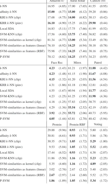
The mean and standard deviation (in parentheses) of the error across the 20 randomized test/training partitions are shown in Table 3. The bold results in each column indicate the classifier with lowest average error; also bolded are any classifiers that were not statistically significantly worse than the classifier with lowest average error.

9. The original data set has 226 samples with 9 classes. As is standard practice with this data set, we removed those classes which contain less than 7 samples.

Amazon-47 Aural Sonar Caltech-101

Face Rec Mirex Patrol

Protein Protein RBF-sim Voting

Figure 1: Similarity matrices of each data set with class divisions indicated by tick marks; black corresponds to maximum similarity and white to zero.

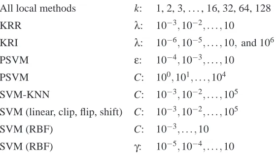
All local methods k: 1, 2, 3, . . . , 16, 32, 64, 128

KRR λ: 10−3_,10−2_{, . . . ,10}

KRI λ: 10−6,10−5, . . . ,10,and 106

PSVM ε: 10−4,10−3, . . . ,10

PSVM C: 100,101, . . . ,104

SVM-KNN C: 10−3,10−2, . . . ,105

SVM (linear, clip, flip, shift) C: 10−3,10−2, . . . ,105

SVM (RBF) C: 10−3, . . . ,10

SVM (RBF) γ: 10−5,10−4, . . . ,10

Table 2: Cross-validation Parameter Choices

The Amazon-47 data set is very sparse with at most four non-zero similarities per row. With such sparse data, one might expect a 1-NN classifier to perform well; indeed for the uniform k-NN

classifier, the cross-validation chose k=1 on all 20 of the randomized partitions. For all of the

local classifiers, the k chosen by cross-validation on this data set was never larger than k=3, and

out of the 20 randomized partitions, k=1 was chosen the majority of the time for all the local

classifiers. In contrast, the global SVM classifiers perform poorly on this sparse data set. The Patrol data set is the next sparsest data set, and the results show a similar pattern. However, the Mirex data set is also relatively sparse, and yet the global classifiers do well, in particular the SVMs that use similarities as features. The Amazon-47 and Patrol data sets do differ from the Mirex data set in that the self-similarities are not always maximal. Whether (and how) this difference causes or correlates the relative differences in performance is an open question.

The Protein data set exhibits large differences in performance, with the statistically significantly best performances achieved by two of the three SVMs that use similarity as features. The reason that similarities on features performs so well while others do so poorly can be seen in the Protein similarity matrix in Figure 1. The first and second classes (roughly the first and second thirds of the matrix) exhibit a strong interclass similarity, and rows belonging to the same class exhibit very similar patterns, thus treating the rows of the similarity matrix as feature vectors provides good discrimination of classes. To investigate this effect, we transformed the entire data set using a radial basis function (RBF) to create a similarity based on the Euclidean distance between rows

of the original similarity matrix, yielding the 213_×213 Protein RBF similarity matrix. One sees

from Table 3 that this transformation increases the performance of classifiers across the board, indicating that this is indeed a better measure of similarity for this data set. Furthermore, after this transformation we see a complete turnaround in performance: for Protein RBF, the SVMs that use similarities as features are among the worst performers (with P-SVM still performing decently), and the basic k-NN does better than the best classifier given the original Protein similarities.

Amazon-47 Aural Sonar Caltech-101

k-NN 16.95 (4.85) 17.00 (7.65) 41.55 (0.95)

affinity k-NN 15.00 (4.77) 15.00 (6.12) 39.20 (0.86)

KRI k-NN (clip) 17.68 (4.75) 14.00 (6.82) 30.13 (0.42)

KRR k-NN (pinv) 16.10 (4.90) 15.25 (6.22) 29.90 (0.44)

Local SDA 16.83 (5.11) 17.75 (7.66) 41.99 (0.52)

SVM-KNN (clip) 17.56 (4.60) 13.75 (7.40) 36.82 (0.60)

SVM-similarities as kernel (clip) 81.34 (4.77) 13.00 (5.34) 33.49 (0.78)

SVM-similarities as features (linear) 76.10 (6.92) 14.25 (6.94) 38.18 (0.78)

SVM-similarities as features (RBF) 75.98 (7.33) 14.25 (7.46) 38.16 (0.75)

P-SVM 70.12 (8.82) 14.25 (5.97) 34.23 (0.95)

Face Rec Mirex Patrol

k-NN 4.23 (1.43) 61.21 (1.97) 11.88 (4.42)

affinity k-NN 4.23 (1.48) 61.15 (1.90) 11.67 (4.08)

KRI k-NN (clip) 4.15 (1.32) 61.20 (2.03) 11.56 (4.54)

KRR k-NN (pinv) 4.31 (1.86) 61.18 (1.96) 12.81 (4.62)

Local SDA 4.55 (1.67) 60.94 (1.94) 11.77 (4.62)

SVM-KNN (clip) 4.23 (1.25) 61.25 (1.95) 11.98 (4.36)

SVM-similarities as kernel (clip) 4.18 (1.25) 57.83 (2.05) 38.75 (4.81)

SVM-similarities as features (linear) 4.29 (1.36) 55.54 (2.52) 42.19 (5.85)

SVM-similarities as features (RBF) 3.92 (1.29) 55.72 (2.06) 40.73 (5.95)

P-SVM 4.05 (1.44) 63.81 (2.70) 40.42 (5.94)

Protein Protein RBF Voting

k-NN 29.88 (9.96) 0.93 (1.71) 5.80 (1.83)

affinity k-NN 30.81 (6.61) 0.93 (1.71) 5.86 (1.78)

KRI k-NN (clip) 30.35 (9.71) 1.05 (1.72) 5.29 (1.80)

KRR k-NN (pinv) 9.53 (5.04) 1.05 (1.72) 5.52 (1.69)

Local SDA 17.44 (6.52) 0.93 (1.71) 6.38 (2.07)

SVM-KNN (clip) 11.86 (5.50) 1.16 (1.72) 5.23 (2.25)

SVM-similarities as kernel (clip) 5.35 (4.60) 1.16 (1.72) 4.89 (2.05)

SVM-similarities as features (linear) 3.02 (2.76) 2.67 (2.12) 5.40 (2.03)

SVM-similarities as features (RBF) 2.67 (2.97) 2.44 (2.60) 5.52 (1.77)

P-SVM 1.86 (1.89) 1.05 (1.56) 5.34 (1.72)

k-NN, suggesting that there are highly correlated samples that bias the classification. In contrast,

for the Amazon-47, Aural Sonar, Face Rec, Mirex, and Patrol data sets there is only a small win by using the KRI or KRR weights, or a statistically insignificant small decline in performance (we

hypothesize this occurs because of overfitting due to the additional parameterλ). On Protein the

KRR error is 1/3 the error of the other weighted methods; this is a consequence of using the pinv rather than other types of spectrum modification, as can be seen from Table 4. The other significant difference between the weighting methods is a roughly 10% improvement in average error on Voting by using the KRR or KRI weights. In conclusion, the use of diverse weights may not matter on some data sets, but can be very helpful on certain data sets.

SVM-KNN was proposed by Zhang et al. (2006) in part as a way to reduce the computations required to train a global SVM using similarities as a kernel, and their results showed that it per-formed similarly to a global SVM. That is somewhat true here, but some differences emerge. For the Amazon-47 and Patrol data sets the local methods all do well including SVM-KNN, but the global methods do poorly, including the global SVM using similarities as a kernel. On the other hand, the global SVM using similarities as a kernel is statistically significantly better than SVM-KNN on Caltech-101, even though the best performance on that data set is achieved by a local method (KRR). From this sampling of data sets, we conclude that applying the SVM locally or globally can in fact make a difference, but whether it is a positive or negative difference depends on the application.

Among the four global SVMs (including P-SVM), it is hard to draw conclusions about the performance of the one that uses similarities as a kernel versus the three that use similarities as features. In terms of statistical significance, the SVM using similarities as a kernel outperforms the others on Patrol and Caltech-101 whereas it is the worst on Amazon-47 and Protein, and there is no clear division on the remaining data sets. Lastly, the results do not show statistically significant differences between using the linear or RBF version of the SVM with similarities as features except for small differences on Face Rec and Patrol.

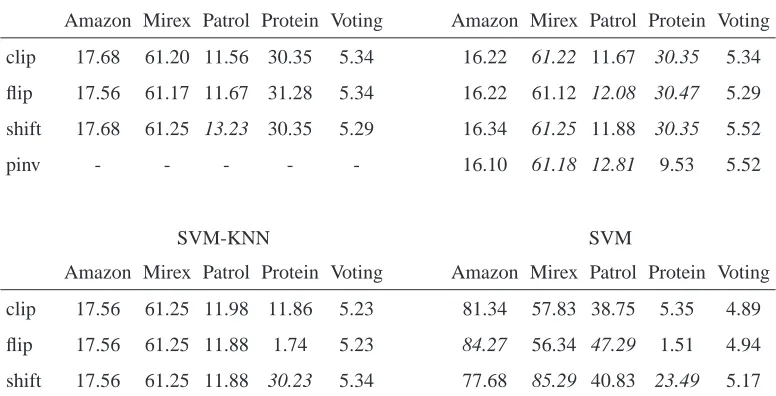
7.4 Clip, Flip, or Shift?

Different approaches to modifying similarities to form a kernel were discussed in Section 2.1. We experimentally compared clip, flip, and shift for the KRI weights, SVM-KNN, and SVM, and flip, clip, shift and pinv for the KRR weights on the nine data sets. Table 4 shows the five data sets for which at least one method showed statistically significantly different results depending on the choice of spectrum modification.

For KRR weights, one sees that the pinv solution is never statistically significantly worse than clip, flip, or shift, which are worse than pinv at least once. For KRI weights, the differences are negligible, but based on average error we recommend clip.

Flip takes the absolute value of the eigenvalues, which is similar to the effect of using SST _(as

KRI KRR

Amazon Mirex Patrol Protein Voting Amazon Mirex Patrol Protein Voting

clip 17.68 61.20 11.56 30.35 5.34 16.22 61.22 11.67 30.35 5.34

flip 17.56 61.17 11.67 31.28 5.34 16.22 61.12 12.08 30.47 5.29

shift 17.68 61.25 13.23 30.35 5.29 16.34 61.25 11.88 30.35 5.52

pinv - - - 16.10 61.18 12.81 9.53 5.52

SVM-KNN SVM

Amazon Mirex Patrol Protein Voting Amazon Mirex Patrol Protein Voting

clip 17.56 61.25 11.98 11.86 5.23 81.34 57.83 38.75 5.35 4.89

flip 17.56 61.25 11.88 1.74 5.23 84.27 56.34 47.29 1.51 4.94

shift 17.56 61.25 11.88 30.23 5.34 77.68 85.29 40.83 23.49 5.17

Table 4: Clip, flip, shift, and pinv comparison. Table shows % test misclassified averaged over 20 randomized test/training partitions for the five data sets that exhibit statistically significant differences between these spectrum modifications. If there are statistically significant dif-ferences for a given algorithm and a given data set, then the worst score, and scores not statistically better, are shown in italics.

8. Conclusions and Some Open Questions

Similarity-based learning is a practical learning framework for many problems in bioinformatics, computer vision, and those regarding human similarity judgement. Kernel methods can be applied in this framework, but similarity-based learning creates a richer set of challenges because the data may not be natively PSD.

In this paper we explored four different approximations of similarities: clipping, flipping, and shifting the spectrum, and in some cases a pseudoinverse solution. Experimental results show small but sometimes statistically significant differences. Based on the theoretical justification and results, we suggest practitioners clip. Flipping the spectrum does create significantly better performance for the original Protein problem because, as we noted earlier, flipping the spectrum has a similar effect to using the similarities as features, which works favorably for the original Protein problem. How-ever, it should be easy to recognize when flip will be advantageous, modify the similarity as we did for the Protein RBF problem, and possibly achieve even better results. Concerning approximating similarities, we addressed the issue of consistent treatment of training and test samples when ap-proximating the similarities to be PSD. Although our linear solution is consistent, we do not argue it is optimal, and consider this issue still open.