Bayesian Co-Training

Bayesian Co-Training

Shipeng Yu [email protected]

Balaji Krishnapuram [email protected]

Business Intelligence and Analytics Siemens Medical Solutions USA, Inc. 51 Valley Stream Parkway

Malvern, PA 19355, USA

R´omer Rosales [email protected]

Yahoo! Labs

4401 Great America Pkwy Santa Clara, CA 95054, USA

R. Bharat Rao [email protected]

Business Intelligence and Analytics Siemens Medical Solutions USA, Inc. 51 Valley Stream Parkway

Malvern, PA 19355, USA

Editor: Carl Edward Rasmussen

Abstract

Co-training (or more generally, co-regularization) has been a popular algorithm for semi-supervised learning in data with two feature representations (or views), but the fundamental assumptions un-derlying this type of models are still unclear. In this paper we propose a Bayesian undirected graphical model for co-training, or more generally for semi-supervised multi-view learning. This makes explicit the previously unstated assumptions of a large class of co-training type algorithms, and also clarifies the circumstances under which these assumptions fail. Building upon new insights from this model, we propose an improved method for co-training, which is a novel co-training ker-nel for Gaussian process classifiers. The resulting approach is convex and avoids local-maxima problems, and it can also automatically estimate how much each view should be trusted to accom-modate noisy or unreliable views. The Bayesian co-training approach can also elegantly handle data samples with missing views, that is, some of the views are not available for some data points at learning time. This is further extended to an active sensing framework, in which the missing (sample, view) pairs are actively acquired to improve learning performance. The strength of active sensing model is that one actively sensed (sample, view) pair would improve the joint multi-view classification on all the samples. Experiments on toy data and several real world data sets illustrate the benefits of this approach.

Keywords: co-training, multi-view learning, semi-supervised learning, Gaussian processes, undi-rected graphical models, active sensing

1. Introduction

if the patient has cancer or not, multiple medical imaging techniques (such as CT, Ultrasound and MRI) might be considered to collect complete characteristic of the patient from different perspec-tives. For learning under such a setting, it has been shown in Dasgupta et al. (2001) that the error rate on unseen test samples can be upper bounded by the disagreement between the classification-decisions obtained from independent characterizations (i.e., views) of the data. Thus, in the web page example, misclassification rate can be indirectly minimized by reducing the rate of disagree-ment between hyperlink-based and content-based classifiers, provided these characterizations are independent conditional on the class label.

As a completely new learning principle, multi-view consensus learning has been the subject of a large body of research recently. This type of methods were originally developed for semi-supervised learning, where class labels are expensive to obtain but unlabeled data are cheap and abundantly available, such as in web page classification. When the data samples can be characterized in multiple views, the disagreement between the class labels suggested by different views can be computed even when using unlabeled data. Therefore, a natural strategy for using unlabeled data to minimize the misclassification rate is to enforce consistency between the classification decisions based on several independent characterizations of the unlabeled samples. For brevity, unless otherwise specified, we shall use the term co-training to describe the entire genre of methods that rely upon this intuition, although strictly it should only refer to the original algorithm of Blum and Mitchell (1998).

In this pioneering paper, Blum and Mitchell introduced an iterative, alternating co-training method, which works in a bootstrap mode by repeatedly adding pseudo-labeled unlabeled samples into the pool of labeled samples, retraining the classifiers for each view, and pseudo-labeling addi-tional unlabeled samples where at least one view is confident about its decision. The paper provided PAC-style guarantees that if (a) there exist weakly useful classifiers on each view of the data, and (b) these characterizations of the sample are conditionally independent given the class label, then the co-training algorithm can use the unlabeled data to learn arbitrarily strong classifiers. Later Balcan et al. (2004) tried to reduce the strong theoretical requirements, and they showed that co-training would be useful if (a) there exist low error rate classifiers on each view, (b) these classifiers never make mistakes in classification when they are confident about their decisions, and (c) the two views are not too highly correlated, in the sense that there would be at least some cases where one view makes confident classification decisions while the classifier on the other view does not have much confidence in its own decision. While each of these theoretical guarantees is intriguing and theoret-ically interesting, they are also rather unrealistic in many application domains. The assumption that classifiers do not make mistakes when they are confident and that of class conditional independence are rarely satisfied in practice. Empirical studies of co-training on many applications show mixed results. See, for instance, Pierce and Cardie (2001) and Kiritchenko and Matwin (2002); Hwa et al. (2003).

A strongly related algorithm is the co-EM algorithm from Nigam and Ghani (2000), which extends the original bootstrap approach of the co-training algorithm to operate simultaneously on all unlabeled samples in an iterative batch mode. Brefeld and Scheffer (2004) used this idea with SVMs as base classifiers, and subsequently in unsupervised learning in Bickel and Scheffer (2005). However, co-EM also suffers from local maxima problems, and while each iteration’s optimization step is clear, the co-EM is not really an expectation maximization algorithm (i.e., it lacks a clearly defined overall log-likelihood that monotonically improves across iterations).

regulariza-tion term that penalizes lack of agreement between the classificaregulariza-tion decisions of the different views. This co-regularization approach has become the dominant strategy for exploiting the intuition be-hind multi-view consensus learning, rendering obsolete earlier alternating-optimization strategies. Krishnapuram et al. (2004) proposed an approach for two-view consensus learning based on simul-taneously learning multiple classifiers by maximizing an objective function which penalized mis-classifications by any individual classifier, and included a regularization term that penalized a high level of disagreement between different views. This co-regularization framework improves upon the co-training and co-EM algorithms by maximizing a convex objective function; however the algo-rithm still depends on an alternating optimization that optimizes one view at a time. This approach was later adapted to two-view spectral clustering in de Sa (2005). The two-view co-regularization approach was subsequently adopted by Sindhwani et al. (2005), Brefeld et al. (2006), Sindhwani and Rosenberg (2008) and Farquhar et al. (2005) for semi-supervised classification and regression based on the reproducing kernel Hilbert space (RKHS). In these approaches a new co-regularization term is added to the objective function which is based on the disagreement of the two views. Repre-senter theorem still holds and solutions can be easily derived by direct optimization. However, it is unclear how to set the regularization parameters (i.e., to control the weight of the co-regularization term). Theoretical analysis of this and other types of algorithms can be found in Balcan and Blum (2006), Sridharan and Kakade (2008), Wang and Zhou (2007) and Wang and Zhou (2010).

Much of these previous work on co-training has been somewhat ad-hoc in nature. Although some algorithms were empirically successful in specific applications, it was not always clear what precise assumptions were made, what was being optimized overall or why they worked well. In this paper we propose a principled undirected graphical model for co-training which we call the Bayesian co-training, and show that co-regularization algorithms provide one way for maximum-likelihood (ML) learning under this probabilistic model. By explicitly highlighting previously un-stated assumptions, Bayesian co-training provides a deeper understanding of the co-regularization framework, and we are also able to discuss certain fundamental limitations of multi-view consen-sus learning. Summarizing our algorithmic contributions, we show that co-regularization is exactly equivalent to the use of a novel co-training kernel for support vector machines (SVMs) and Gaus-sian processes (GP), thus allowing one to leverage the large body of available literature for these algorithms. The kernel is intrinsically non-stationary, that is, the level of similarity between any pair of samples depends on all the available samples, whether labeled or unlabeled, thus promoting semi-supervised learning. Therefore, this approach is significantly simpler and more efficient than the alternating-optimization that is used in previous co-regularization implementations. Further-more, we can automatically estimate how much each view should be trusted, and thus accommodate noisy or unreliable views.

The basic idea of Bayesian co-training was published in a short conference paper by Yu et al. (2008). In the current paper we have all the derivation details and more discussions to its related models. More importantly, we extend the Bayesian co-training model to handle data samples with missing views (i.e., some views are missing for certain data samples), and introduce a novel ap-plication called the active sensing. This makes the current paper significantly different from its conference version.

can-cer diagnosis perspective, active learning is equivalent to choosing patients to do a biopsy such that the tumor is correctly diagnosed (benign/malignant), whereas active sensing is targeting at collect-ing (the not-yet-been-collected) medical imagcollect-ing features (of, e.g., CT, Ultrasound and MRI) from some patients such that all the patients can be better diagnosed. This is important, since a patient does not undergo all possible tests at once (due to various side effects such as radiation and con-trast), but these tests are selected based on the evidence collected up to a particular point. This is normally referred to as differential diagnosis. Another example is in land mine detection in a sensor network. We may have different types of sensors (as different views) deployed at one location, but some sensors may not be available for all locations due to high cost. So active sensing is to decide which location and which type of sensor we should additionally consider to achieve better detection accuracy. Formulated within the Bayesian co-training framework, two approaches will be discussed for efficiently choosing the (sample, view) pair, based on the mutual information (involving various random variables) and on the predictive uncertainty, respectively.

This active sensing problem is similar to active feature acquisition—see, for example, Melville et al. (2004) and Bilgic and Getoor (2007)—but there is a clear difference. Previous feature acqui-sition only considers one sample at a time, that is, when one sample is in consideration, the other samples will not be affected. But in active sensing, one actively acquired (sample, view) pair will improve the classification performance of all the unlabeled samples via a co-training setting. A related yet different problem was considered in Krause et al. (2008) to identify the optimal spatial locations for placing a single type of sensor to model spatially varying phenomena; however, this work addressed the use of a single type of sensor, and do not consider the scenario of multiple views. The rest of the paper is organized as follows. We introduce the Bayesian co-training model in Section 2, covering both the undirected graphical model and various marginalizations. Co-training kernel will be discussed in detail to highlight the insight of the approach. The model is extended to handle missing views in Section 4, and this provides the basics for the active sensing solution. The active sensing problem is discussed in Section 5, in which we provide two methods for deciding which incomplete samples should be further characterized, and which sensors should be deployed on them. Experimental results are provided in Section 6, including both some toy problems and real world problems on web page classification and differential diagnosis. We conclude with a brief discussion and future work in Section 7.

2. Bayesian Co-Training

We start from an undirected graphical model for single-view learning with Gaussian processes, and then present Bayesian co-training which is a new undirected graphical model for multi-view learning.

2.1 Single-View Learning with Gaussian Processes

co-y

₁

f

₁

(x

₁(1)

₎

…

…

f

_c

(x

₁

)

f

_c

(

x

₂

)

f

_c

(x

_n

)

y

₂

y

_n

f

₁

(x

₂(1)

₎

_f

1

(x

n(1)

)

f

₂

(x

₁(2)

₎

_f

2

(x

2(2)

)

f

2

(x

n(2)

)

y

₁

f(x

₁

)

…

y

₂

y

_n

f(x

₂

)

f (x

_n

)

(a)

(b)

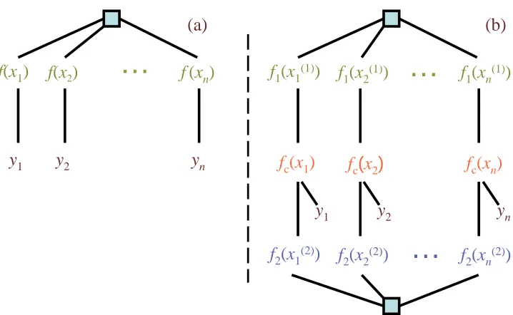
Figure 1: Factor graph for (a) one-view and (b) two-view models.

variance functionκis assumed to take a parametric (and usually stationary) form (e.g., the squared exponential functionκ(xi,xj) =exp(−_2ρ12kxi−xjk2)withρ>0 a width parameter).

In a single-view, supervised learning scenario, an output or target yiis given for each observation xi (e.g., for regression yi _∈Rand for classification yi _{∈ {−}1,+1_}). In the GP model we assume there is a latent function f underlying the output,

p(yi_|xi) =

Z

p(yi_|f,xi)p(f)d f =

Z

p(yi_|f(xi))p(f)d f,

with the GP prior p(f) =

GP

(h,κ). Given the latent function f , for regression p(yi|f(xi))takes a Gaussian noise model

N

(yi|f(xi),σ2), withσ>0 a parameter for the noise level; for classification p(yi_|f(xi))takes the form of a sigmoid functionλ(yif(xi)). For instance for GP logistic regression, we haveλ(z) = (1+exp(₋z))−1_{. See Rasmussen and Williams (2006) for more details on this.}

The dependency structure of the single-view GP model can be shown as an undirected graph as in Figure 1(a). The maximal cliques of the graphical model are the fully connected nodes {f(x1), . . . ,f(xn)} and the pairs {yi,f(xi)}, i=1, . . . ,n. Therefore, the joint probability of ran-dom variables f=_{f(xi)}and y={yi}is defined as

p(f,y) =1 Zψ(f)

n

∏

i=1

ψ(yi,f(xi)),

with potential functionsψ(f) =exp(₋1 2f⊤K−

1_{f), and}1

ψ(yi,f(xi)) =

(

exp(₋₂1_σ2kyi−f(xi)k2) for regression,

λ(yif(xi)) for classification.

(1)

The normalization factor Z hereafter is defined such that the joint probability sums to 1.

f

₁

f

₂

f

_c

y

f

₁

f

_m

f

_c

y

f

₂

…

2-views

multi-views

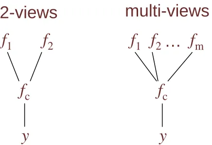
Figure 2: Factor graph in the functional space for 2-view and multi-view learning.

2.2 Undirected Graphical Model for Multi-View Learning

In multi-view learning, suppose we have m different views of a same set of n data samples. Let x(j)_{i ∈} Rdj _{be the features for the ith sample obtained using the jth view, where d}

jis the dimensionality of the input space for view j. Note that subscripts index the data sample, and superscripts (with round brackets) index the view. Then the vector xi,(x(1)i , . . . ,x

(m)

i )is the complete representation of the ith data sample, and x(j),(x(₁j), . . . ,x(nj))represents all sample observations for the jth view. As in the single-view learning, let y= [y1, . . . ,yn]⊤ _{be the output where yi is the single output assigned to} the ith data point.

One can certainly concatenate the multiple views of the data into a single view, and apply a single-view GP model. But the basic idea of multi-view learning is to introduce one function per view, which only uses the features from that specific view to make predictions. Multi-view learning then jointly optimizes these functions such that they come to a consensus. From a GP perspective, let fj denote the latent function for the jth view (i.e., using features only from view j), and let fj∼

GP

(0,κj)be its GP prior in view j with covariance functionκj. Since one data sample i has only one single label yi even though it has multiple features from the multiple views (i.e., latent function value fj(x(ij))for view j), the label yishould depend on all of these latent function values for data sample i.

The challenge here is to make this dependency explicit in a graphical model. We tackle this problem by introducing a new latent function, the consensus function fc, to ensure conditional independence between the output y and the m latent functions_{fj_}for the m views. See Figure 1(b) for the undirected graphical model for multi-view learning. At the functional level, the output y depends only on fc, and latent functions_{fj}depend on each other only via the consensus function fc(see Figure 2 for the factor graphs for 2-view and multi-view cases). That is, the joint probability is defined as:

p(y,fc,f1, . . . ,fm) = 1

Zψ(y,fc) m

∏

j=1

ψ(fj,fc), (2)

respectively. The graphical model leads to the following factorization:

p(y,fc,f1, . . . ,fm) = 1 Z

n

∏

i=1

ψ(yi,fc(xi)) m

∏

j=1

ψ(fj)ψ(fj,fc). (3)

Here the within-view potential ψ(fj) specifies the dependency structure within each view j, and the consensus potentialψ(fj,fc) describes how each latent function fj is related to the consensus function fc. With a GP prior for each of the m views, we can define the following potentials:

ψ(fj) =exp

−1 2f

⊤ jK−j1fj

, ψ(fj,fc) =exp

−kfj−fck 2 2σ2_j

, (4)

where Kj is the covariance matrix of view j, that is, Kj(xk,xℓ) =κj(x_k(j),x(_ℓj)), and σj >0 is a scalar which quantifies how apart the latent function fjis from the consensus function fc. It is seen that the within-view potentials only rely on the intrinsic structure of each view, that is, through the covariance matrix in a GP setting. Finally, the output potentialψ(yi,fc(xi))is defined the same as that in (1) for regression or for classification.

The most important potential function in Bayesian co-training is the consensus potential, which simply defines an isotropic multivariate Gaussian for the difference of fj and fc, that is, fj−fc∼

N

(0,σ2

jI). This can also be interpreted as assuming a conditional isotropic Gaussian for fj with the consensus fc being the mean. Alternatively if fc is of interest, the joint consensus potentials effectively define a conditional Gaussian prior for fc, fc|f1, . . . ,fm, as

N

(µc,σ2cI)where

µ_c=σ2_c

∑

j

fj

σ2 j

, σ2_c =

∑

j 1

σ2 j

−1

. (5)

One can easily verify that this is a product of Gaussian distributions, with each Gaussian being

N

(fc_|fj,σ2jI).2 This indicates that, given the latent functions{fj}m_j=1, the posterior mean of the consensus function fc is a weighted average of these latent functions, and the weight is given by the inverse variance (i.e., the precision) of each consensus potential. The higher the variance, the smaller the contribution to the consensus function. In the following we callσ2_j the view variance for view j. In this paper these view variances are taken as parameters of the Bayesian co-training model, but one can also assign a prior (e.g., a Gamma prior) to them and treat them instead as hidden variables. We will discuss the consensus potential and the view variances in more details in Section 3.

In (3) we assume the output y is available for all the n data samples. More generally we consider semi-supervised multi-view learning, in which only a subset of data samples have outputs available. This is actually the setting for which co-training and multi-view learning were originally motivated (Blum and Mitchell, 1998). Formally, let nl be the number of data samples which have outputs available, and let nu be the number of data samples which do not. We still keep n=nl+nu to be the total number of data samples. Under this setting, we only have outputs available for nl samples, that is, y_l= [y1, . . . ,ynl]⊤.

In the functional space, the undirected graphical model for semi-supervised multi-view learning is the same as in Figure 2. The joint probability is also the same as in (2). In the ground network,

since the output vector y_lis only of length nl, the joint probability is now:

p(y_l,fc,f1, . . . ,fm) = 1 Z

nl

∏

i=1

ψ(yi,fc(xi)) m

∏

j=1

ψ(fj)ψ(fj,fc). (6)

Note that the product of output potentials contains only that of the nl labeled data samples, and that fc=_{fc(xi)_}n

i=1and fj={fj(x(j)i )}ni=1are still of length n. Unlabeled data samples contribute to the joint probability via the within-view potentialsψ(fj)and consensus potentialsψ(fj,fc). All the potentials are defined similarly as in (4). In the following we will mainly discuss this more interesting setting.

3. Inference and Learning in Bayesian Co-Training

In this section we discuss inference and learning in the proposed model, assuming first that there is no missing data in any of the views (the setting with missing data will be discussed in Sec-tion 4). Instead of working with the undirected graphical model directly, we show different types of marginalizations under this model. The standard inference task is that of inferring y from the observed data, that is, obtaining p(y); however, in order to gain insight into the proposed model and co-training, we explore different marginalizations. All marginalizations lead to standard Gaussian process inference with different latent function at consideration, but interestingly, these different marginalizations show different insights of the proposed undirected graphical model. One advan-tage of the marginalizations is that it allows us to see that many existing multi-view learning models are actually special cases of the proposed framework. In addition, this Bayesian interpretation helps us understand both the benefits and the limitations of co-training. For clarity we put the derivations into Appendix A.

3.1 Marginal 1: Co-Regularized Multi-View Learning

Our first marginalization focuses on the joint probability distribution of the m latent functions, when the consensus function fc is integrated out. This would lead to a GP model in which the latent functions are the view specific functions f1, . . . ,fm. Taking the integral of (3) over fc (and ignoring the output potential for the moment), we obtain the joint marginal distribution as follows after some mathematics (for derivations see Appendix A.1):

p(f1, . . . ,fm) = 1 Zexp

(

−1₂ m

∑

j=1

f⊤_jK−_j1fj− 1 2

∑

_j<k

"

kfj−fkk2

σ2 jσ2k

∑

ℓ

1

σ2

ℓ

#)

. (7)

It can be seen that the negation of the logarithm of this marginal recovers the regularization terms in the co-regularized multi-view learning (see, e.g., Sindhwani et al., 2005; Brefeld et al., 2006). In particular, we have

−log p(f1, . . . ,fm) = 1 2

m

∑

j=1

f⊤_j K−_j1fj+ 1 2

∑

_j<k

"

kfj−fkk2

σ2 jσ2k

∑

ℓ

1

σ2

ℓ

#

+log Z

=1 2

m

∑

j=1

Ωj(fj) + 1 2

1

∑ℓ 1

σ2

ℓ

∑

j<k

where Ωj(fj),f⊤j K−j1fj regularizes the functional space of each individual view j, and the loss function L(fj,fk),kfj−fkk2

σ2

jσ2kmeasures the disagreement of every pair of the function outputs, inversely weighted by the product of the corresponding variances. The higher the varianceσ2_j of view j, the less the contribution view j brings to the overall loss. We refer to this as variance-sensitive co-regularized multi-view learning. Note that unlike the formulation in Brefeld et al. (2006) where the disagreements are only with respect to the unlabeled data, here we regularize the disagreements of all data samples. From the GP perspective, (7) actually defines a joint multi-view prior for the m latent functions,(f1, . . . ,fm)∼

N

(0,Λ−1), where Λis a mn×mn precision matrix with block-wise definition:

Λ(j,j) =K−_j1+ 1

∑ℓ 1

σ2

ℓ

∑

k₆=j 1

σ2 jσ2k

I, Λ(j,j′) =₋ 1

∑ℓ 1

σ2

ℓ

1

σ2 jσ2j′

I, j′₆= j. (8)

It is seen that the block-wise precision matrix for view j has contributions from all the other views. When we take into account the observed output variable y, we can also easily derive the joint marginal of y with all the latent functions f1, . . . ,fm. For instance for regression, the marginal distri-bution turns out to be (recall thatσ2is the variance parameter in the output potential for regression):

p(y,f1, . . . ,fm) = 1 Zexp

(

−_2ρσ1 2

∑

j

∑n

i=1(yi−fj(xi))2

σ2 j

−1₂

∑

j

f⊤_jK−_j1fj− 1 2ρ

∑

_j<k

kfj−fkk2

σ2 jσ2k

)

. (9)

Hereρ,_σ12+∑j_σ12

j is the sum of all the inverse variances, including the regression variance.

Max-imizing this marginal distribution is equivalent to solving a minimization problem in co-regularized multi-view learning with least square loss. It is seen that the least square loss with respect to the jth latent function fj is inversely weighted by the varianceσ2j, which indicates again that a higher variance leads to less contribution to the total loss.

3.2 Marginal 2: The Co-Training Kernel

The joint multi-view kernel defined in (8) is interesting, but it has a large dimension and is difficult to work with. A more interesting kernel can be obtained if we instead integrate out all the m latent functions f1, . . . ,fmin (3). This leads to a standard (transductive) Gaussian process model, with fc being the latent function realizations, and GP prior being p(fc) =

N

(0,Kc)where

Kc=

"

∑

j

(Kj+σ2jI)−1

#−1

. (10)

co-training, and it also means that this kernel lacks the marginalization property and can only be used in a transductive setting.

This kernel definition is crucial to Bayesian co-training, and in the following we call Kc the co-training kernel for multi-view learning. This marginalization reveals the previously unclear insight of how the kernels from different views are combined together in a multi-view learning framework. This allows us to transform a multi-view learning problem into a single-view prob-lem, and simply use the co-training kernel Kc to solve GP classification or regression. Since this marginalization is equivalent to (7),3we end up with solutions that are largely similar to any other co-regularization algorithm, but however a key difference is the Bayesian treatment contrasting pre-vious ML-optimization methods.

Formulation (10) can also be viewed as a kernel design for transductive multi-view learning, namely, the inverse of the co-training kernel is the sum of the inverse of all individual kernels, corrected by the view specific variance term. Higher variance leads to less contribution to the overall training kernel. In a transductive setting where the data are partially labeled, the co-training kernel between labeled data is also dependent on the unlabeled data. Hence the proposed co-training kernel, by the design in (10), can be used for semi-supervised GP learning (Zhu et al., 2003).

Additional benefits of the co-training kernel include the following:

• With fixed hyperparameters (e.g.,σ2_j), the co-training kernel avoids repeated alternating op-timizations with respect to the different views fj, and directly works with a single consensus view fc. This reduces both time complexity and space complexity (since we only maintain Kc in memory) of multi-view learning.

• While other alternating optimization algorithms might converge to local minima (because they optimize, not integrate), the single consensus view guarantees the global optimal infer-ence solution for multi-view learning since it marginalizes other latent functions and leads to a standard GP inference model.

• Even if all the individual kernels are stationary, Kc is in general non-stationary. This is because the inverse-covariances are added and then inverted again.

3.3 Marginal 3: Individual View Learning with Side-Information

In Bayesian co-training model we can also focus on one particular view j by marginalizing all the other views and the consensus view. This is particularly interesting if there is one view that is of the main interest (e.g., it provides the most useful features, or it has the least missing features), and we want to understand how the other views influence this view in the inference process. This can be done by integrating out the other latent functions fk, k6= j, in (7), and it will lead to another GP formulation with fj being the latent function. Since (7) represents a jointly Gaussian distribution, we obtain fj∼

N

(0,Cj), where

C−_j1=K−_j1+

"

σ2 jI+

∑

k6=j

Kk+σ2kI

−1

#−1

. (11)

See Appendix A.3 for the derivation. This can be intuitively understood as that the precision matrix of the individual view, C−_j1, is the sum of its original precision matrix and the contributions from other views, weighted by the inverse of the variance. Therefore ifσ2

k is big for some view k, its contribution to the other views will be compromised. Hence, if one particular view is of interest, we can encode the additional information from the other views into the kernel for the interested view.

Another benefit of this marginalization is the possibility of introducing an inductive inference scheme (rather than transductive as in Section 3.2)—given a new test data x_∗, we try to make a prediction of y_∗ if the jth view x(_∗j) is available. Inspired by Yu et al. (2005), let us define

αj= [αj1, . . . ,αjn]⊤∈Rnsuch that fj(x) =∑ni=1αjiκj(x(j),x(_ij))(this is also motivated by the Rep-resenter theorem). On the training data, this yields fj =Kjαj. From (11) we can see that this re-parameterization leads to a co-training prior forαj asαj∼

N

(0,K−j1CjK−j1). At testing time when we have the posterior ofαj, y_∗ can be approximated by fj(x_∗) =∑ni=1αjiκj(x(_∗j),x(_ij)). This approach is particularly interesting in the case that one of the views is known to be predictive (i.e., the other views are “side” information to help this primary view), or test data often come with fea-tures only in a specific view (since the feafea-tures from the other views would be disregarded at testing time).

3.4 Optimization of Hyperparameters

One of the advantages of Bayesian co-training is that each view j has a view-specific variance term

σ2

j to quantify how far the latent function fj is apart from the consensus view fc. In particular, a larger value ofσ2_j implies less confidence on the observation of evidence provided by the jth view. In the perspective of kernel design, this leads to a lesser weight on the kernel Kj. Thus when some views of the data are better at predicting the output than the others, they are weighted more while forming consensus opinions. These variance terms are hyperparameters of the Bayesian co-training model.

To optimize these variance terms together with other hyperparameters involved in each covari-ance function (e.g., parameterρ>0 in the Gaussian kernelκ(xi,xj) =exp(−ρkxi−xjk2)), we can use the type II maximum likelihood method (sometimes called evidence approximation), which maximizes the marginal likelihood with respect to each of these hyperparameters. For simplicity we put the derivation and detailed equations in Appendix B. For more details on the type II maximum likelihood in the GP setting, please refer to Rasmussen and Williams (2006).

3.5 Discussions

The proposed undirected graphical model provides better understanding of multi-view learning al-gorithms. In each of the marginalizations, we end up with a standard GP model for some latent functions (i.e., _{f1, . . . ,fm} in Marginal 1, fc in Marginal 2, and fj in Marginal 3). This simpli-fies learning and inference under the proposed model. Under a transductive setting, the co-training kernel in (10) indicates that Bayesian co-training is equivalent to single-view learning with a spe-cially designed (non-stationary) kernel. This is also the preferable way of working with multi-view learning since it avoids alternating optimizations at the inference step.

co-training kernel Kc encodes the similarity of two data samples with multiple views, and thus can be used directly in spectral clustering.

We would also like to point out the limitations of the proposed consensus-based learning, which are shared by co-training as proposed by Blum and Mitchell (1998) and many other multi-view learning algorithms. As mentioned before, the consensus-based potentials in (4) can be interpreted as defining a Gaussian prior (5) to fc, where the mean is a weighted average of the m individual views. This averaging indicates that the value of fcis never higher (or lower) than that of any single view. While the consensus-based potentials are intuitive and useful for many applications, they are limited for some real world problems where the evidence from different views should be additive (or enhanced) rather than averaging. For instance, when a radiologist is making a diagnostic decision about a lung cancer patient, he or she might look at both the CT image and the MRI image. If either of the two images gives a strong evidence of cancer by that image alone, he or she can make a decision based on a single view (and thus, ignoring the other image completely); if either of the images only gives a moderate evidence (i.e., from a single-view learner which ignores the other image), it would be beneficial to look at both images (i.e., to consider both views), and the final evidence of cancer after observing both images should be higher (or lower, depending on the specific scenario) than either of them if observed individually. It’s clear that in this scenario the multiple views are reinforcing or weakening each other, not averaging. While all the previously proposed co-training and co-regularization algorithms have thus far been based on enforcing consensus between the views explicitly or implicitly, we make this clear from the graphical model perspective, and allow effective tailoring of the view importance from the training data. As part of future work, it would be interesting to explore the possibility of going beyond consensus-based multi-view learning.

4. Bayesian Co-Training with Missing Views

In the previous two sections we assume that the input data are complete, that is, all the views are observed for every data sample. However for many real-world problems, the features could be incomplete or missing for various reasons. For instance, in cancer diagnosis we cannot ask every patient to take all the available imaging tests (e.g., CT, PET, Ultrasound, MRI) for the final diagnosis, so some views (i.e., imaging tests) are missing for certain patients. In this section we extend Bayesian co-training to the case where there are missing (sample, view) pairs in the input data (which can happen both in labeled data and in unlabeled data). The three marginalizations will also be discussed. To the best of our knowledge, this is the first elegant framework to account for the missing views in the multi-view learning setting.

Let each view j be observed for a subset of nj ≤n samples, and let Ij denote the indices of these samples in the whole sample set (including labeled and unlabeled data). Note that under this notation, the single-view kernel matrix Kj for view j is of size nj×nj, which are defined over the subset of samples denoted by indicatorIj. From the co-training kernel perspective, the difficulty here is to combine the kernels of different sizes together from different views, if at all possible.

with missing views, which is very similar to Figure 1(b). The joint probability can be defined as:

p(y_l,fc,f1, . . . ,fm) = 1 Z

nl

∏

i=1

ψ(yi,fc(xi)) m

∏

j=1

ψ(fj)ψ(fj,fc), (12)

where fc=_{fc(xi)_}n

i=1∈Rn, and fj={fj(xi(j))}i_∈Ij ∈Rnj. Note that fj is only realized on a subset of samples and is of length nj (instead of n). The within-view potential ψ(fj) is defined via the GP prior, ψ(fj) =exp(−1₂f⊤j K−j1fj), where Kj ∈Rnj×nj is the covariance matrix for view j; the consensus potentialψ(fj,fc)is defined as follows:

ψ(fj,fc) =exp −k

fj−fc(Ij)k2 2σ2

j

!

, (13)

in which fc(Ij)takes the length-nj subset of vector fc with indices given inIj. In other words, the consensus potentials is defined such that

ψ(fj(xi),fc(xi)) =exp − 1

2σ2_j fj(xi)−fc(xi)

2

!

, i_∈Ij.

The idea here is to define the consensus potential for view j using only the data samples observed in view j. The other data samples with missing view information for view j are treated as hidden (or integrated out) in this potential definition. As before,σj>0 quantifies how far the latent function fj is apart from fc. Note that the smaller njis, the less the contribution of view j to the overall graphical model.4 Next we look at the three marginalizations to gain more insight about this graphical model.

4.1 Co-Regularization with Missing Views

It is straightforward to derive all the marginalizations of Bayesian co-training with missing views. For the co-regularization marginal, a simple calculation leads to the following joint distribution for the m latent functions:

p(f1, . . . ,fm) = 1 Zexp

(

−1₂ m

∑

j=1

f⊤_jK−_j1fj− 1

2

∑

_{j<k x∈}

∑

_Ij∧Ik

"

[fj(x)−fk(x)]2

σ2 jσ2k

∑

ℓ:x∈Iℓ

1

σ2

ℓ

# )

.

As in the Bayesian training with fully observed views, this provides an equivalent form to co-regularized multi-view learning. The first part regularizes the functional space of each view, and the second part constrains that every pair of views need to agree on the outputs for co-observed samples (inversely weighted by view variances and the sum of inverse variances of the views in which the sample is observed). This is very intuitive and naturally extends the joint distribution in (7). If view j and view k do not share any data sample (i.e., no data sample has features from both view j and view k), the view pair (j,k)will not contribute to the joint distribution.5 _{A joint probability} distribution involving output y_l can also be derived which takes a similar form as in (9).

4. Also note that after hyperparameter learning,σjmight not fully represent how strongly each view j contributes to

the consensus, since the contribution also depends on the number of available data njin the view j.

(a)

(b)

y₁

f_c(x₁)

f_c(x_j)

fc(xn) f₁(x₁(1)₎

…

f₁(x_j(1)₎

f₁(x_n(1)₎

…

f₂(x₁(2)₎

f₂(x_j(2)₎

f2(xn(2)) f(x₁)

…

f(x_j)

f(x_n) y_n y₁

y_j

y_j

y_n

f_c(x_k) f₁(x_k(1)_{) f}

2(xk(2))

y_k

…

…

…

…

f(x_k) y_k

…

…

x₁(1)

xj(1)

x_k(1)

x₁(1)

xj(1)

xk(1)

x_n(1)

x₁(2)

x_j(2)

x_k(2)

xn(2)

…

…

…

…

…

…

…

…

…

x_n(1)

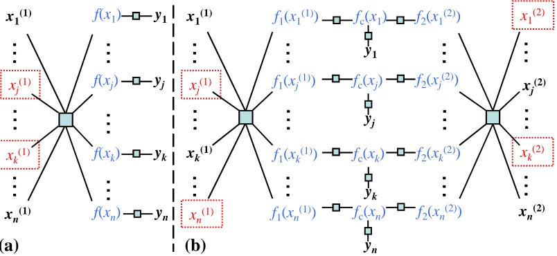
Figure 3: Factor graphs for Bayesian co-training with missing views, for (a) one-view and (b) two-view problems. Observed variables are marked as dark/bold, and unobserved ones are marked as red/non-bold, including functions f1,f2,fc(blue/non-bold). Unobserved vari-ables in a dotted box (such as x(1)_j ) are potential observations for active sensing (see Section 5). All labels y are denoted as observed in the graph, but this is not required.

4.2 Co-Training Kernel with Missing Views

We can also derive a co-training kernel Kc by integrating out all the latent functions{fj}in (12). This leads to a Gaussian prior p(fc) =

N

(0,Kc), with

Kc=Λ−1

c , Λc= m

∑

j=1 Aj,

where each Ajis a n×n matrix defined as

Aj(Ij,Ij) = (Kj+σ2jI)−1,and 0 otherwise. (14) That is, Aj is an expansion of the one-view information matrix(Kj+σ2jI)−1to the full size n×n, with the other (unindexed) entries filled with 0. It is easily seen that such a kernel Kc is indeed positive definite, as long as each one-view kernel Kj is positive definite and at least there are two views sharing one data sample. We also callΛcthe co-training precision matrix. Very importantly, we note that one additional observation of a (sample, view) pair will affect all the elements of the co-training kernel. In other words, the kernel value for a pair of samples is potentially changed even when a third (unrelated) object is further characterized by an additional sensor.6 This property mo-tivates us to do active feature acquisition (or active sensing) in the Bayesian co-training framework. Section 5 will discuss this in detail.

6. Note that the marginalizations in Section 4.2 and Section 4.1 are still equivalent (since they come from the same un-derlying graphical model), despite the fact that additional (sample, view) pair influences the kernels (with dimension

4.3 Individual View Learning with Missing Views

If one particular view j is of interest, we can also integrate out the consensus view and all the other views, leading to a GP prior for view j, fj∼

N

(0,Cj), with the precision matrix being

C−_j1=K−_j1+

σ2

jI+Λc\j(Ij,Ij)−1

−1

.

Here we extract the (Ij,Ij) sub-matrix from the leave-one-view-out co-training precision matrix

Λc\j, which is defined asΛc\j=∑k₆=jAk. Each Akis defined as in (14). This marginalization allows us to, for example, measure how much benefit every other view brings to the interested view. An important fact to realize here is that with an observed (sample, view) pair from another view k, even if this sample is not observed in the primarily interested view j, the kernel of the view j will still be affected so long asIj∧Ik6=/0. One can also introduce the inductive GP inference as in Section 3.3 under this setting.

4.4 Discussion

Bayesian co-training with missing views provides an elegant framework to combine information from multiple views or multiple data sources together, even when different subsets of data samples are measured in different views. For learning and inference, we still prefer using the co-training kernel with the second marginalization due to its simplicity.

We note that the definition of the consensus potentials in (13) implies that the influence of the different pairs of views has been factored into a product. As a consequence, the view-pairs are combined in a linear manner. A way to go beyond this is by using higher-order potentials.

A higher order potential definition ψ(f1, ...,fm,fc), which combines f1, ...,fm simultaneously, would produce a richer combination of views, but often at the expense of increased inference/computational complexity. It is not clear how to achieve this effect with standard co-training.

Since one observation of a (sample, view) pair will affect the overall co-training kernel, we can derive a framework for active sensing, which aims to actively select the best pair for feature acquisition or sensing. This active sensing problem is different from active learning where the goal is to select the best pair for labeling. We discuss this idea in detail in the next section.

5. Active Sensing in Bayesian Co-Training

In active sensing, we are interested in selecting the best unobserved (sample, view) pair for sensing, or for view acquisition, which will improve the overall classification performance. In this section we will focus on logistic regression loss for binary classification. For active sensing we mainly discuss an approach based on the mutual information framework, which measures the expected information gain after observing an additional (sample, view) pair. Another approach based on the predictive uncertainty is also briefly discussed in Section 5.5.

In the following let

D

O and

D

U denote the observed and unobserved (sample, view) pairs, respectively. Recall that under the second marginalization in which only the consensus function fc is of primary interest, the Bayesian co-training model for binary classification reduces to

p(y_l,fc) = 1 Zψ(fc)

nl

∏

i=1

where y_l contains the binary labels for the nl labeled samples,ψ(fc) is defined via the co-training kernel asψ(fc) =exp₋1₂f⊤_cK−_c1fc , andψ(yi,fc(xi))is the output potentialλ(yifc(xi))withλ(_·) the logistic function. The log marginal likelihood of the output y_l under this model, conditioned on the input data X,_{x(_ij)_}and model parametersΘ, is:

L

,log p(y_l|X,Θ) =log

Z

p(y_l|fc,Θ)p(fc_|X,Θ)dfc₋log Z

=log

Z nl

∏

i=1

λ(yifc(xi))_·exp

−1₂f⊤_cK−_c1fc

dfc₋log Z.

5.1 Laplace Approximation

To calculate the mutual information we need to calculate the differential entropy of the consensus view function fc. With co-training kernel and the logistic regression loss, Laplace approximation can be applied to approximate the a posteriori distribution of fc as a Gaussian distribution. The a posteriori distribution of fc, p(fc_|

D

O,yl,Θ)∝p(yl|fc,Θ)p(fc|

D

O,Θ), is approximately

N

(ˆfc,(∆post)−1), (15)

where ˆfcis the maximum a posteriori (MAP) estimate of fc, and the a posteriori precision matrix is

∆post=K−c1+Φ, (16)

with Φ the Hessian of the negative log-likelihood. It turns out thatΦ is a diagonal matrix, with

Φ(i,i) =ηi(1−ηi)whereηi=λ(ˆfc(xi)). The differential entropy of fcunder this Laplace approxi-mation is

H(fc) =₋n

2log(2πe)− 1

2log det(∆post), where det(_·)denotes the matrix determinant.

5.2 Mutual Information for Active Sensing

Remind that x(_ij)denote the features in the jth view for the ith sample. In active sensing, the mutual information (MI) between the consensus view function fc and the unobserved (sample, view) pair x(_ij)∈

D

U is the expected decrease in entropy of fcwhen x(ij)is observed,

I(fc,x(ij)) =E[H(fc)]−E[H(fc|x(j)i )] =− 1

2log det(∆post) + 1

2E[log det(∆ x(i,j) post )],

where the expectation is with respect to p(x(_ij)_|

D

O,yl), the distribution of the unobserved (sample, view) pair given all the observed pairs and available outputs. ∆x(i_post,j) is the a posteriori precision matrix, derived from (16), after one pair x(_ij)is observed.

The maximum MI criterion has been used before to identify the “best” unlabeled sample in active learning (MacKay, 1992). Here we adopt this criterion and choose the unobserved pair which maximizes MI:

(i∗,j∗) =arg max x(ij)∈DU

I(fc,x(_ij)) =arg max x(ij)∈DU

5.3 Density Modeling

In order to calculate the expectation in (17), we need a conditional density model for the unobserved pairs, that is, p(x(j)_{i |}

D

O,yl). This of course depends on the type of the features in each view, and for our applications we use a special Gaussian mixture model (GMM). This model has the nice property that all the marginals are still GMMs, and yet is not too flexible like the full GMM. One can certainly define other density models based on the applications.

For a m-view input data x= (x(1), . . . ,x(m)), let the joint input density be

p(x(1), . . . ,x(m)) =p(y= +1)p(x(1), . . . ,x(m)|y= +1) +p(y=₋1)p(x(1), . . . ,x(m)|y=₋1),

and each conditional density takes a component-wise factorized GMM form, that is,

p(x(1), . . . ,x(m)_|y= +1) =

∑

c

π+ c

∏

j

N

(x(j)_|µ+(j)c ,Σ+(c j)),

p(x(1), . . . ,x(m)_|y=₋1) =

∑

c

π− c

∏

j

N

(x(j)_|µc−(j),Σ−c(j)).

Here, for the positive class, µ+(c j) and Σ+(c j) are the mean and covariance matrix for view j in component c, andπ+_c >0, ∑_cπ+_c =1 are the mixture weights. For the negative class we use sim-ilar notations. Note that although the conditional density for each mixture component is decou-pled for different views, the joint conditional density is not.7 Under this model, the joint density p(x(1), . . . ,x(m))is also a GMM, and any marginal (conditioned on y or not) density is still a GMM, for example, p(x(j)_|y= +1) =∑_cπ+

c

N

(x(j)|µ +(j)

c ,Σ+(c j)). Now it is easy to calculate p(x(_ij)_|

D

O,yl). Let x

(O)

i be the set of observed views for xi, we need to distinguish two different settings. When the label yiis available, for example, yi= +1, we have

p(x(j)_{i |}

D

O,yl) =p(x (j) i |x

(O)

i ,yi= +1) =

∑

c

π+(j)

c (x(O)_i ) ·

N

(x_i(j)|µ+(j)c ,Σ+(c j)), (18)

which is again a GMM model, with the mixing weights being

π+(j)

c (x(O)i ) =π+c

∏k∈O

N

(x (k) i |µ

+(k) c ,Σ+(k)c ) p(x(O)_i |yi= +1) .

When the label yi is not available, we need to integrate out the labeling uncertainty and compute

p(x(_ij)_|

D

O,yl) =p(x (j) i |x

(O) i )

=p(yi= +1)p(x_i(j)_|x(O)_i ,yi= +1) +p(yi=₋1)p(x(_ij)_|x(O)_i ,yi=₋1),

which is a GMM model as well, as can be seen from (18).

5.4 Expectation Calculation

We are now ready to compute the expectation in (17). The a posteriori precision matrix after one (sample, view) pair x(j)_i is observed,∆x(i_post,j), can be calculated as

∆x(i,j) post = (K

x(i,j)

c )−1+Φ=Ax(ij ,j)+

∑

k6=j

Ak+Φ, (19)

where Kx(ic ,j)and Ax(ij ,j)are the new Kc and Aj matrices after the new pair is observed. Based on (14), to calculate Ax(i_j ,j) we need to recalculate the kernel for the jth view, Kj, after an additional pair x(j)_i is observed. This is simply done by adding one row and column to the old Kj as:

Kx(i_j ,j)=

Kj bj b⊤_j aj

,

where aj=κj(x(j)i ,x (j)

i )∈R, and bj∈Rnj has theℓth entry asκj(x(j)_ℓ ,x(ij)). Then from (14), the non-zero part of Ax(i_j ,j)is calculated as

Kx(i_j ,j)+σ2_jI

−1

=

Kj+σ2jI bj b⊤_j aj+σ2j

−1

=

Γ

j+λjΓjbjb⊤j Γj −λjΓjbj −λjb⊤_jΓj λj

, (20)

using the block-matrix inverse formula, whereΓj= (Kj+σ2jI)−1andλj= _a 1

j+σ2j−b⊤jΓjbj.

As seen from (19) and (20), it is difficult to directly calculate the expectation in (17). Since for any matrix Q,E[log det(Q)]_≤log det(E[Q])due to the concavity of log det(_·), we alternatively take the upper bound log det(E[∆x(i_post,j)])as the selection criteria and also take the risk that the best pair (i,j) that optimizes log det(E[∆_postx(i,j)])doesn’t necessarily optimize E[log det(∆x(i_post,j))]. From (19) and (20), this reduces to computingE[λj],E[λjbj]andE[λjbjb⊤j], where the expectations are with respect to p(x(_ij)_|

D

O,y), a GMM model (cf. Section 5.3). In general one needs to calculate these expectations numerically, as different kernel functions lead to different integrals. As another approximation one might assume each of the GMM component is a point-mass such that the mean is used for the calculation.

5.5 Discussion

The mutual information based approach directly measures the expected information gain for every (sample, view) pair. A different (and simpler) approach is based on the predictive uncertainty, in which the most uncertain sample (after the current classifier is trained) is selected for view acqui-sition. This approach was taken for a different problem in Melville et al. (2004). This uncertainty (i.e., predictive variance) is estimated as the diagonal entries of the a posteriori covariance matrix (∆post)−1, as seen from (15). However it is not clear what view to acquire for this sample (if more than one view is missing for the sample). The advantage of this approach is that no density modeling is necessary for unobserved views.

6. Experiments

co-training models with the original co-training method proposed by Blum and Mitchell (1998), and several single-view learning algorithms. Since this co-training algorithm—sometimes we call it the canonical co-training algorithm—was proposed for classification problems, we focus on classi-fication in this section and compare all the methods with the logistic regression loss. We show both problems where co-training works and does not work (i.e., is not better compared to the single-view learning counterpart).

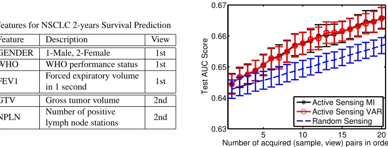
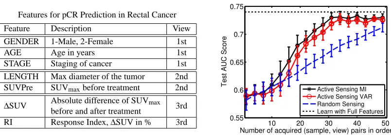
In the second part we evaluate the active sensing algorithms in the Bayesian co-training setting. We are given a classification task with missing views, and at each iteration we are allowed to select an unobserved (sample, view) pair for sensing (i.e., feature acquisition). The proposed methods are compared with random sensing in which a random unobserved (sample, view) pair is selected for sensing.

6.1 Toy Examples for Bayesian Co-Training

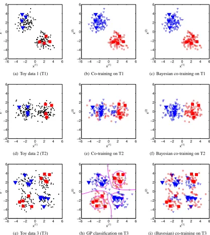
First of all, we show some 2D toy classification problems to visualize the co-training result in Figure 4. We assume each of these 2D problems is a two-view problem, in which one view only contains one single feature. Canonical co-training is applied by iteratively training one classifier based on one view, adding the most confident unlabeled data from one view to the training pool of the other classifier, and retraining each classifier till convergence (i.e., no confident unlabeled data can be added further). In Bayesian co-training we use the squared exponential covariance function as mentioned in Section 2, and the widthρis set to 1/√2 which yields the optimal performance.

Our first example is a two-Gaussian case with mean (2,₋2) and(₋2,2), where either feature x(1) or x(2) can be used alone to fully solve the problem (Figure 4(a)). This is an ideal case for co-training, since: 1) each single view is sufficient to train a classifier, and 2) both views are con-ditionally independent given the class labels. Therefore we see that both canonical co-training and Bayesian co-training yield the same perfect result (Figure 4(b),(c)).

For the second toy data (Figure 4(d)) we assume the two Gaussians are aligned to the x(1)-axis (with mean(2,0)and(₋2,0)). In this case the feature x(2)is totally irrelevant to the classification problem. The canonical co-training fails here (Figure 4(e)) since when we add labels using the x(2) feature , noisy labels will be introduced and expanded to future training. The Bayesian co-training model can handle this situation since we can adapt the weight of each view and penalize the feature x(2)(Figure 4(f)).

The third toy data follows an XOR shape where the data from four Gaussians (with mean(2,2), (₋2,2), (2,₋2), (₋2,₋2)) lead to a binary classification problem that is not linearly separable (Figure 4(g)). In this case both the two assumptions mentioned above are violated, and neither canonical nor Bayesian co-training will work (Figure 4(i)).8 On the other hand, a supervised GP classification model with squared exponential covariance function can easily recover the non-linear underlying structure (see Figure 4(h)). This indicates that the learning a multi-view classifier for this problem with the current co-training type algorithms will not succeed. From a kernel design perspective, the consensus based co-training kernel Kc is not suitable for this type of problem.

In summary, these toy problems indicate that when co-training works, Bayesian co-training performs better than or at least as well as canonical training models. But since Bayesian co-training is fundamentally a kernel design for a single-view supervised learning, it will not work when the problem calls for more flexible kernel form (e.g., in Figure 4(g)).

−6 −4 −2 0 2 4 6 −6 −4 −2 0 2 4 6 x(1) x (2)

(a) Toy data 1 (T1)

−6 −4 −2 0 2 4 6

−6 −4 −2 0 2 4 6 x(1) x (2)

(b) Co-training on T1

−6 −4 −2 0 2 4 6

−6 −4 −2 0 2 4 6 x(1) x (2)

(c) Bayesian co-training on T1

−6 −4 −2 0 2 4 6

−6 −4 −2 0 2 4 6 x(1) x (2)

(d) Toy data 2 (T2)

−6 −4 −2 0 2 4 6

−6 −4 −2 0 2 4 6 x(1) x (2)

(e) Co-training on T2

−6 −4 −2 0 2 4 6

−6 −4 −2 0 2 4 6 x(1) x (2)

(f) Bayesian co-training on T2

−6 −4 −2 0 2 4 6

−6 −4 −2 0 2 4 6 x(1) x (2)

(g) Toy data 3 (T3)

−6 −4 −2 0 2 4 6

−6 −4 −2 0 2 4 6 −0.5 −0.5 −0.5 −0.5 0 0 0 0 0 0 0.5 0.5 0.5 0.5 0.5 x(1) x (2)

(h) GP classification on T3

−6 −4 −2 0 2 4 6

−6 −4 −2 0 2 4 6 x(1) x (2)

(i) (Bayesian) co-training on T3

# TRAIN+2/-10 # TRAIN+4/-20

MODEL AUC F1 AUC F1

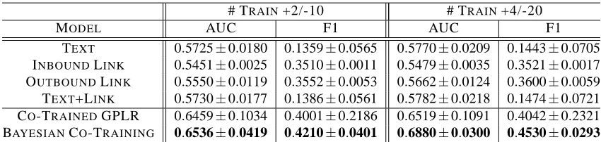
TEXT 0.5725_±0.0180 0.1359_±0.0565 0.5770_±0.0209 0.1443_±0.0705 INBOUNDLINK 0.5451_±0.0025 0.3510_±0.0011 0.5479_±0.0035 0.3521_±0.0017 OUTBOUNDLINK 0.5550_±0.0119 0.3552_±0.0053 0.5662_±0.0124 0.3600_±0.0059 TEXT+LINK 0.5730_±0.0177 0.1386_±0.0561 0.5782_±0.0218 0.1474_±0.0721 CO-TRAINEDGPLR 0.6459_±0.1034 0.4001_±0.2186 0.6519_±0.1091 0.4042_±0.2321 BAYESIANCO-TRAINING 0.6536_±0.0419 0.4210_±0.0401 0.6880_±0.0300 0.4530_±0.0293

Table 1: Results for Citeseer with different numbers of labeled training data (positive/negative). The first three lines are supervised learning results using only the single-view features. The fourth line shows the supervised learning results by combining features from all the three views. The fifth and sixth lines are the co-training results. Bold face indicates the best performance.

MODEL # TRAIN+2/-2 # TRAIN+4/-4

AUC F1 AUC F1

TEXT 0.5767_±0.0430 0.4449_±0.1614 0.6150_±0.0594 0.5338_±0.1267 INBOUNDLINK 0.5211_±0.0017 0.5761_±0.0013 0.5210_±0.0019 0.5758_±0.0015 TEXT+LINK 0.5766_±0.0429 0.4443_±0.1610 0.6150_±0.0594 0.5336_±0.1267 CO-TRAINEDGPLR 0.5624_±0.1058 0.5437_±0.1225 0.5959_±0.0927 0.5737_±0.1203 BAYESIANCO-TRAINING 0.5794_±0.0491 0.5562_±0.1598 0.6140_±0.0675 0.5742_±0.1298

Table 2: Results for WebKB with different numbers of labeled training data (positive/negative). The first two lines are supervised learning results using only the single-view features. The third line shows the supervised learning results by combining features from both views. The fourth and fifth lines are the co-training results. Bold face indicates the best performance.

6.2 Bayesian Co-Training for Web Page Classification

We use two sets of linked documents for our experiment. The main purpose of these empirical studies is to show the benefit of the proposed Bayesian co-training method compared to single-view learning and the canonical co-training algorithms, and also highlight the limitations of co-training type algorithms. As will be seen later, we show one case that co-training works, in which case Bayesian co-training yields the best performance; we also show one case that co-training does not improve over the single-view counterpart, in which case Bayesian co-training is slightly better than canonical training. As the training kernel based approach is equivalent to the adaptive co-regularized multi-view learning (since they are based on the same underlying graphical model), we do not include a separate line of results for the co-regularization methods.