Logistic Stick-Breaking Process

(1)

Logistic Stick-Breaking Process

Lu Ren LR@EE.DUKE.EDU

Lan Du LD53@EE.DUKE.EDU

Lawrence Carin LCARIN@EE.DUKE.EDU

Department of Electrical and Computer Engineering Duke University

Durham, NC 27708, USA

David B. Dunson DUNSON@STAT.DUKE.EDU

Department of Statistical Science Duke University

Durham, NC 27708, USA

Editor: David Blei

Abstract

A logistic stick-breaking process (LSBP) is proposed for non-parametric clustering of general spatially- or temporally-dependent data, imposing the belief that proximate data are more likely to be clustered together. The sticks in the LSBP are realized via multiple logistic regression func-tions, with shrinkage priors employed to favor contiguous and spatially localized segments. The LSBP is also extended for the simultaneous processing of multiple data sets, yielding a hierarchical logistic stick-breaking process (H-LSBP). The model parameters (atoms) within the H-LSBP are shared across the multiple learning tasks. Efficient variational Bayesian inference is derived, and comparisons are made to related techniques in the literature. Experimental analysis is performed for audio waveforms and images, and it is demonstrated that for segmentation applications the LSBP yields generally homogeneous segments with sharp boundaries.

Keywords: Bayesian, nonparametric, dependent, hierarchical models, segmentation

1. Introduction

One is often interested in clustering data that have associated spatial or temporal coordinates. This problem is relevant in a diverse set of applications, such as climatology, ecology, environmental health, real estate marketing, and image analysis (Banerjee et al., 2003). The available spatial or temporal information may be exploited to help infer patterns, clusters or segments in the data. To simplify the exposition, in the following discussion we focus on exploiting spatial information, although when presenting results we also consider temporal data (Fox et al., 2008).

(2)

of-ten one must pre-define the total number of segments/clusters. Further, such graphical techniques are not readily extended to the joint analysis of multiple spatially dependent data sets, with this of interest for the simultaneous analysis of multiple images.

To consider clustering in a nonparametric Bayesian manner, the Dirichlet process (DP) (Black-well and MacQueen, 1973) has been employed widely (Antoniak, 1974; Escobar and West, 1995; Rasmussen, 2000; Beal et al., 2002). Assume we are given N data points,{yn}Nn=1, with yn

repre-senting a feature vector; each feature vector is assumed drawn from a parametric distribution F(θn).

For each yn, the DP mixture model is represented as

yn|θn∼F(θn), θn|G iid

∼G, G|α0,G0∼DP(α0G0),

whereα0is a non-negative precision parameter and G0is the base probability measure. Sethuraman

(1994) developed an explicit method for constructing a draw G from a DP:

G=

∞

∑

k=1

πkδθ∗

k, πk=Vk

k−1

∏

k′₌₁

(1−Vk′), V_kiid∼Beta(1,α₀), θ_k∗iid∼G0. (1) The precision parameterα0controls the number of sticks that have appreciable weights, with these

weights defining the probability that different θn share the same “atoms”θk∗. Since α0 plays an

important role in defining the number of significant stick weightsπk, we typically place a gamma

prior onα0to allow the data to inform about its value.

The assumption within the DP that the data are exchangeable is generally inappropriate when one wishes to impose knowledge of spatial information (in which each ynhas an associated spatial

location). For example, the data may be represented as{yn,sn}N_n₌₁, in which ynis again the feature

vector and snrepresents the spatial location of yn. Provided with such spatial information, one may

wish to explicitly impose the belief that proximate data are more likely to be clustered together. The spatial location snmay be readily considered as an appended feature, and the modified

fea-ture vectors (data) may then be analyzed via traditional clustering algorithms, like those discussed above. For example, the spatial coordinate has been considered explicitly in recent topic models (Cao and Li, 2007; Wang and Grimson, 2007; Gomes et al., 2008) when applied in image analysis. These previous studies seek to cluster visual words, with such clustering encouraged if the features are spatially proximate. However, these methods may produce spurious clusters that are introduced to better characterize the spatial data likelihood instead of the likelihood of the features condition-ally on spatial location (Park and Dunson, 2009). In addition, such approaches require a model for the spatial locations, which is not statistically coherent as these locations are typically fixed by design, and there may be additional computational burden for this extra component.

(3)

As an alternative to the above approaches, a kernel stick-breaking process (KSBP) has been proposed (Dunson and Park, 2007), imposing that clustering is more probable if two feature vectors are close in a prescribed (general) space, which may be associated explicitly with spatial position for image processing applications (An et al., 2008). With the KSBP, rather than assuming exchangeable data, the G in(1)becomes a function of spatial location:

Gs=

∞

∑

k=1

πk(s;Vk,Γk,ψ)δθ∗

k,

πk(s;Vk,Γk,ψ) =VkK(s,Γk;ψ)

k−1

∏

k′₌₁

1−Vk′K(s,Γ_k′;ψ),

Vk∼Beta(1,α0), θ∗k ∼G0, Γk∼H0,

(2)

where K(s,Γk;ψ)represents a kernel distance between the feature-vector spatial coordinate s and a

local basis locationΓk associated with the kth stick. As demonstrated when presenting results, the

KSBP generally does not yield smooth segments with sharp boundaries.

Instead of thresholding K latent Gaussian processes (Duan et al., 2007) to assign a feature vector to a particular parameter, we introduce a novel non-parametric spatially dependent prior, called the logistic stick-breaking process (LSBP), to impose that it is probable that proximate feature vectors are assigned to the same parameter. The new model is constructed based on a hierarchy of spa-tial logistic regressions, with sparseness-promoting priors on the regression coefficients. With this relatively simple model form, inference is performed efficiently with variational Bayesian analysis (Beal, 2003), allowing consideration of large-scale problems. Further, for reasons discussed below, this model favors contiguous segments with sharp boundaries, of interest in many applications. The model developed in the paper (Chung and Dunson, 2009), based on a probit stick-breaking process, is most closely related to the proposed framework; the relationships between LSBP and the model (Chung and Dunson, 2009) are discussed in detail below.

In addition to exploiting spatial information when performing clustering, there has also been recent research on the simultaneous analysis of multiple tasks. This is motivated by the idea that multiple related tasks are likely to share the same or similar attributes (Caruana, 1997; An et al., 2008; Pantofaru et al., 2008). Exploiting the information contained in multiple data sets (“tasks”), model-parameter estimation may be improved (Teh et al., 2005; Pantofaru et al., 2008; Sudderth and Jordan, 2008). Therefore, it is desirable to employ multi-task learning when processing multiple spatially-dependent data (e.g., images), this representing a second focus of this paper.

Motivated by previous multi-task research (Teh et al., 2005; An et al., 2008), we consider the problem of simultaneously processing multiple spatially-dependent data sets. A separate LSBP prior is employed for each of the tasks, and all LSBPs share the same base measure, which is drawn from a DP. Hence, a “library” of model parameters—atoms—is shared across all tasks. This construction is related to the hierarchical Dirichlet process (HDP) (Teh et al., 2005), and is referred to here as a hierarchical logistic stick-breaking process (H-LSBP).

(4)

The remainder of the paper is organized as follows. In Section 2 we introduce the logistic stick-breaking process (LSBP) and discuss its connections with other models. We extend the model to the hierarchical LSBP (H-LSBP) in Section 3. For both the LSBP and H-LSBP, inference is performed via variational Bayesian analysis, as discussed in Section 4. Experimental results are presented in Section 5, with conclusions and future work discussed in Section 6.

2. Logistic Stick-breaking Process (LSBP)

We first consider spatially constrained clustering for a single data set (task). Assume N sample points {Dn}n=1,N, where Dn = (yn,sn), with yn representing the nth feature vector and sn its

as-sociated spatial location. We draw a set of candidate model parameters, and the probability that a particular space-dependent data sample employs a particular model parameter is defined by a spatially-dependent stick-breaking process, represented by a kernel-based logistic-regression.

2.1 Model Specifications

Assume an infinite set of model parameters{θ_k∗}∞_k₌₁. Each observation yn is drawn from a

para-metric distribution F(θn), withθn∈ {θk∗}∞k=1. To indicate which parameter in{θk∗}∞k=1is associated

with the nth sample, a set of indicator variables Zn={zn1,zn2, . . . ,zn∞} are introduced for each

Dn, and all the indicator variables are equal to zero or one. Given Zn, data Dn is associated with

parameterθ∗_k if znk=1 and znˆk=0 for ˆk<k.

The Zn are drawn from a spatially dependent density function, encouraging that proximate Dn

will have similar Zn, thereby encouraging spatial contiguity. This may be viewed in terms of a

spatially dependent stick-breaking process. Specifically, let pk(sn)define the probability that znk=

1, with 1−pk(sn)representing the probability that znk=0; the spatial dependence of these density

functions is made explicit via sn. The probability that the kth parameter is selected in the above

model isπk(sn) =pk(sn)∏k_ˆk=1−1[1−p_ˆk(sn)], which is of the same form as a stick-breaking process

(Ishwaran and James, 2001) but extends to a spatially dependent mixture model, represented as

Gsn= ∞

∑

k=1

πk(sn)δθ∗

k, πk(sn) =pk(sn)

k−1

∏

ˆk=1

[1−p_ˆk(sn)].

Here each pk(sn)is defined in terms of a logistic link function (other link functions may also be

employed, such as a probit). Specifically, we consider Nc discrete spatial locations{ˆsi}N_i₌₁c within

the domain of the data (e.g., the locations of the samples in Dn). To allow the weights of the different

mixture components to vary flexibly with spatial location, we propose a kernel logistic regression for each break of the stick, with

log

pk(sn)

1−pk(sn)

=gk(sn) = Nc

∑

i=1

wkiK(sn,ˆsi;ψk) +wk0, (3)

where gk(sn)is the linear predictor in the logistic regression model for the kth break and position

sn, and

K(sn,ˆsi;ψk) =exp h

−ksn−ˆsik 2

ψk

i

is a Gaussian kernel measuring closeness of locations snand ˆsi, as in a radial basis function model

(5)

[wk0,wk1, . . . ,wkNc]

′_{. A sparseness-promoting prior is chosen for the components of W}

k, such that

only a relatively small set of wkiwill have non-zero (or significant) amplitudes; those spatial regions

for which the associated amplitudes are non-zero correspond to regions for which a particular model parameter is expected to dominate in the segmentation (this is similar to the KSBP in (2), which also has spatially localized kernels). The indicator variables controlling allocation to components are then drawn from

znk∼Bernoulli[σ gk(sn)

],

whereσ(g) =1/[1+exp(−g)]is the inverse of the logit link in (3).

There are many ways that such sparseness promotion may be constituted, and we have consid-ered two. As one choice, one may employ a hierarchical Student-t prior as applied in the relevance vector machine (Tipping, 2001; Bishop and Tipping, 2000; Bishop and Svens´en, 2003):

wki∼N(wki|0,λ_ki−1)Gamma(λki|a0,b0),

where shrinkage is encouraged with a0=b0=10−6(Tipping, 2001). Alternatively, one may

con-sider a “spike-and-slab” prior (Ishwaran and Rao, 2005). Specifically,

wki∼νk

N

(0,λ−1_k ) + (1−νk)δ0, νk∼Beta(νk|c0,d0).

The expression δ0 represents a unit point measure concentrated at zero. The parameters (c0,d0)

are set such that νk is encouraged to be close to zero (or we simply fix νk = _c₀c₊0_d₀), enforcing

sparseness inwk; the parameterλkis again drawn from a gamma prior, with hyperparameters set to

allow a possibly large range in the non-zero values of wki, and therefore these are not set as in the

Student-t representation. The advantage of the latter model is that it explicitly imposes that many of the components ofwk are exactly zero, while the Student-t construction imposes that many of the

coefficients are close to zero. In our numerical experiments on waveform and image segmentation, we have employed the Student-t construction.

Note that parameterθ∗_k is associated with ans-dependent function gk(s), and there are K−1

such functions. The model is constructed such that within a contiguous spatial/temporal region, a particular parameterθ∗_k is selected, with these model parameters used to generate the observed data. There are two key components of the LSBP construction: (i) sparseness promotion on the wki,

and (ii) the use of a logistic link function to define space-dependent stick weights. As discussed fur-ther in Section 2.2, these concepts are motivated by the idea of making a particular space-dependent LSBP stick weightπk(s) =σ(gk(s))∏k′_<_k[1−g′_k(s)]near one within a localized region in space (motivating the sparseness prior on the weights), while also yielding contiguous segments with sharp boundaries (manifested via the logistic).

It is desirable to allow flexibility in the kernel parameter ψ, as this will influence the size of segments that are encouraged (discussed further below). Hence, for each k we draw

ψk=ψ∗rk, rk∼Mult(1/τ, . . . ,1/τ),

withΨ∗={ψ∗_j}τ_j₌₁a library of possible kernel-size parameters; rk is an index for the one non-zero

(6)

weights{wk}k=1,K−1, with a similar representation used for a spike-and-slab prior; note that Gsis

defined simultaneously for all spatial locations. The model parameters{θ_k∗}∞_k₌₁are assumed drawn from the measure H.

In practice we usually truncate the LSBP to K sticks, as in a truncated stick-breaking process (Ishwaran and James, 2001). With a truncation level K specified, if znk=0 for all k=1, . . . ,K−1,

then znK=1 so thatθn=θ∗K. The VB analysis yields an approximation to the marginal likelihood

of the observed data, which can be used to evaluate the effect of K on the model performance. When presenting results we consider simply setting K to a large value, and also test the model performance with K initialized to different values.

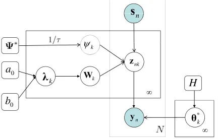
Figure 1 shows the graphical form of the model (using a Student-t sparseness prior), in which

Ψ∗ represents the discrete set of kernel-width candidates,ψk is the kernel width selected for the

kth stick, and the prior H takes on different forms depending upon the application. In Figure 1 the

1/τ emphasizes that the candidate kernel widths are selected with uniform probability over theτ candidates inΨ∗.

s

\

n

s

nk z

0 a

k

\

k W

f

k

Ȝ

0 a

b

H

*

k

ș n

y

0 b

f f

Figure 1: Graphical representation of the LSBP.

2.2 Discussion of LSBP Properties and Relationship to Other Models

The proposed model is motivated by the work (Sudderth and Jordan, 2008), in which multiple draws from a Gaussian process (GP) are employed. Candidate model parameters are associated with each GP draw, and the GP draws serve to constitute a nonparametric gating network, associating particular model parameters with a given spatial position. In the model (Sudderth and Jordan, 2008) the spatial correlation associated with the GP draws induces spatially contiguous segments (a highly spatially correlated gating network), and this may be related to a spatially-dependent stick-breaking process. However, use of the GP produces computational challenges. The proposed LSBP model also manifests multiple space-dependent functions (here gk(r)), with associated candidate

model parameters{θ_k∗}k=1,K. Further, we constitute a spatially dependent gating network that has a

stick-breaking interpretation. However, a different and relatively simple procedure is proposed for favoring spatially contiguous segments with sharp boundaries.

At each locationswe have a stick-breaking process, with the probability of selecting model pa-rameters θ∗_k defined as πk(s) = σ(gk(s))∏k′_<_k[1 − σ(g_k′(s))]. Recall that

(7)

stick weightπ1(s)for allssufficiently distant from those locations ˆsiwith non-zero w1i. Further, if w1i≫0,σ(g1(s))≈1 forsin the “neighborhood” of the associated location ˆsi; the neighborhood

size is defined byψ1. Hence, those{sˆi}i=1,Ncwith associated large{w1i}i=1,Nc define localized re-gions as a function ofsover which parameterθ∗₁is highly probable, with locality defined by kernel scale parameterψ1. For those regions of sfor whichπ1(s) is not near one, there is appreciable

probability 1−π1(s)that model parameters{θk∗}k=2,Kmay be used.

Continuing the generative process, model parametersθ₂∗are probable whereπ2(s) =σ(g2(s))[1−

π1(s)]≈1. The latter occurs in the vicinity of thosesthat are distant from ˆsiwith large associated

w1i (i.e., where 1−π1(s)≈1), while also being near ˆsi with large w2i (i.e., whereσ(g2(s))≈1).

We again underscore that w20impactsπ2(s)for alls.

This process continues for increasing k, and therefore it is probable that as k gets large all or almost allswill be associated with a large stick weight, or a large cumulative sum of stick weights, such that parametersθ∗_k become improbable for large k and alls.

Key characteristics of this construction are the clipping property of the logistic link function, and the associated fast rise of the logistic. The former imposes that there are contiguous regions (segments) over which the same model parameter has near-unity probability of being used. This encouraging of homogeneous segments is also complemented by sharp segment boundaries, mani-fested by the fast rise of the logistic. The aforementioned “clipping” property is clearly not distinct to logistic regression. It would apply as well to other binary response link functions, which can be any CDF for a continuous random variable. For example, probit links (Chung and Dunson, 2009) would have the same property, though the logistic has heavier tails than the probit so may have slightly different clipping properties. We have here selected the logistic link function for computa-tional simplicity (it is widely used, for example, in the relevance vector machine Tipping 2001, and we borrow related technology). It is interesting to see how the segmentation realizations differ with the form of link function, with this to be considered in future research.

To give a more-detailed view of the generative process, we consider a one-dimensional exam-ple, which in Section 5 will be related to a problem with real data. Specifically, consider a one-dimensional signal with 488 discrete sample points. In this illustrative example Nc=98, defined

by taking every fifth sample point for the underlying signal. We wish to examine the generative process of the LSBP prior, in the absence of data. For this illustration, it is therefore best to use the spike-and-slab construction, since without any data the Student-t construction will with high probability make all wki≈0 (when considering data, and evaluating the posterior, a small fraction

of these coefficients are pulled away from zero, via the likelihood function, such that the model fits the data; we reconsider this in Section 5). Further, again for illustrative purposes, we here treat

{wk0}k=1,K as drawn from a separate normal distribution, not from the spike-and-slab prior used

for all other components ofwk. This distinct handling of{wk0}k=1,K has been found unnecessary

when processing data, as the likelihood function again imposes constraints on{wk0}k=1,K. Hence

this form of the spike-and-slab prior onwkis simply employed to illuminate the characteristics of

LSBP, with model implementation simplifying when considering data.

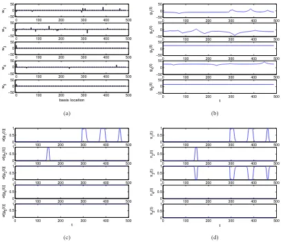
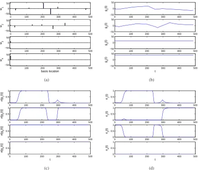
In Figure 2 we plot representative draws for wk, gk(s), σ(gk(s)) and πk(s), for the

one-dimensional signal of interest. In this illustrative example each νk is drawn from Beta(1,10) to

encourage sparseness, and those non-zero coefficients are drawn from

N

(0,λ), withλfixed to cor-respond to a standard deviation of 15 (we could also draw eachλkfrom a gamma distribution). Each

bias term wk0is here drawn iid from

N

(0,λ). We see from Figure 2 that the LSBP naturally favors

(8)

0 100 200 300 400 500 −50

0 50

w1

0 100 200 300 400 500

−50 0 50

w2

0 100 200 300 400 500

−50 0 50

w3

0 100 200 300 400 500

−50 0 50

w4

0 100 200 300 400 500

−50 0 50 w5 basis location (a)

0 100 200 300 400 500

−50 0 50

g1

(t)

0 100 200 300 400 500

−50 0 50

g2

(t)

0 100 200 300 400 500

−50 0 50

g3

(t)

0 100 200 300 400 500

−50 0 50

g4

(t)

0 100 200 300 400 500

−50 0 50 g5 (t) t (b)

0 100 200 300 400 500

0 0.5 1 σ [g1 (t)]

0 100 200 300 400 500

0 0.5 1 σ [g2 (t)]

0 100 200 300 400 500

0 0.5 1 σ [g3 (t)]

0 100 200 300 400 500

0 0.5 1 σ [g4 (t)]

0 100 200 300 400 500

0 0.5 1 σ [g5 (t)] t (c)

0 100 200 300 400 500

0 0.5 1

π1

(t)

0 100 200 300 400 500

0 0.5 1

π2

(t)

0 100 200 300 400 500

0 0.5 1

π3

(t)

0 100 200 300 400 500

0 0.5 1

π4

(t)

0 100 200 300 400 500

0 0.5 1 π5 (t) t (d)

Figure 2: Example draw from a one-dimensional LSBP, using a spike-and-slab construction for model-parameter sparseness. (a)wk, (b) gk(t), (c)σk(t), (d)πk(t)

typical draw, where we note that for k≥4 the probability ofθ∗_kbeing used is near zero. While Figure 2 represents a typical LSBP draw, one could also envision other less-desirable draws. For example, if w10≫0 thenπ1(s)≈1 for alls, implying that the parametersθ1∗ is used for alls(essentially

no segmentation). Other “pathological” draws may be envisioned. Therefore, we underscore that the data, via the likelihood function, clearly influences the posterior strongly, and the pathological draws supported by the prior in the absence of data are given negligible mass in the posterior.

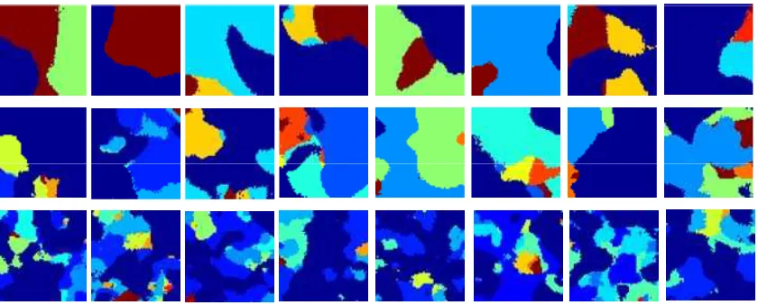
As further examples, now for two-dimensional signals, Figure 3 considers example draws as a function of the kernel parameterψk. These example draws were manifested via the same process

used for the one-dimensional example in Figure 2, now extending sto two dimensions. Figure 3 also shows the dependence of the size of the segments on the kernel parameter ψk, which has

motivated the learning of ψk in a data-dependent manner (based on a finite dictionary of kernel

(9)

Figure 3: Samples drawn from the spatially dependent LSBP prior, for different (fixed) choices of kernel parametersψ, applied for each k within the LSBP. In row 1 ψ=15; in row 2 ψ=10; and in row 3ψ=5. In these examples the spike-and-slab prior has been used to impose sparseness on the coefficients{wk}k=1,K−1.

3. Hierarchical LSBP (H-LSBP)

Multi-task learning (MTL) is an inductive transfer framework (Caruana, 1997), with the goal of improving modeling performance by exploiting related information in multiple data sets. We here employ MTL for joint analysis of multiple spatially dependent data sets, yielding a hierarchical logistic stick-breaking process (H-LSBP). This framework models each individual data set (task) with its own LSBP draw, while sharing the same set of model parameters (atoms) across all tasks, in a manner analogous to HDP (Teh et al., 2005). The set of shared model atoms are inferred in the analysis.

The spatially-dependent probability measure for task m, Gm, is drawn from a LSBP with base

measure G0, and G0 is shared across all M tasks. Further, G0 is drawn from a Dirichlet process

(Blackwell and MacQueen, 1973), and in this manner each task-dependent LSBP shares the same set of discrete atoms. The H-LSBP model is represented as

ymn|θmn∼F(θmn), θmn|Gm∼Gm,

Gm|{G0,a0,b0,Ψ∗} ∼LSBP(G0,a0,b0,Ψ∗),

G0|γ,H∼DP(γH).

Note that we are assuming a Student-t construction of the sparseness prior within the LSBP, defined by hyperparameters a0and b0.

Assume task m∈ {1, . . . ,M}has Nmobservations, defining the data

Dm={Dm1, . . . ,Dm(Nm)}. We introduce a set of latent indicator variables

tm={tm1, . . . ,tm∞}for each task, with

tmk iid

∼

∞

∑

l=1

(10)

where βl corresponds to the lth stick weight of the stick-breaking construction of the DP draw

G0=∑∞_l₌₁βlδθ∗

l. The indicator variables tmkestablish an association between the observations from each task and the atoms{θ_l∗}∞_l₌₁shared globally; hence the atomθ_t∗_mk is associated with LSBP gk

for task m. Accordingly, we may write the probability measure Gm, for position smn, in the form

Gsmn=

∞

∑

k=1

πmk(smn)δθ∗ tmk.

Note that it is possible that in such a draw we may have the same atom used for two different LSBP

gk. This doesn’t pose a problem in practice, as the same type of segment (atom) may reside in

multiple distinct spatial positions (e.g., of an image), and the different k with the same atom may account for these different regions of the data.

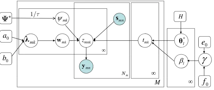
A graphical representation of the proposed hierarchical model is depicted in Figure 4. As in the single-task LSBP discussed in Section 2, a uniform prior is placed on the discrete elements ofΨ∗, and the precision parameterγfor the Dirichlet process is assumed drawn from a gamma distribution Ga(e0,f0). In practice we truncate the number of sticks used to represent G0, employing L−1

draws from the beta distribution, and the length of the Lth stick isβL=1−∑L_l₌₁−1βl (Ishwaran and

James, 2001). We also set a truncation level K for each Gm, analogous to truncation of a traditional

stick-breaking process.

We note that one may suggest drawing L atomsθ_l∗∼H, for l=1, . . . ,L, and then simply

as-signing each of these atoms in the same way to each of K=L gk in the M LSBPs associated with

the M images under test. Although there are K functions gk in the LSBP, as a consequence of the

stick-breaking construction, those with small index k are more probable to be used in the generative process. Therefore, the process reflected by (4) serves to re-order the atoms in an task-dependent manner, such that the important atoms for a given task occur with small index k. In our experi-ments, we make K<L, since the number of different segments/atoms anticipated for any given task

is expected to be small relative to the library of possible atoms{θ_l∗}L

l=1available across all tasks.

mk

\ s_mn H

mnk

z

mk

w *

l

ș

f mk

Ȝ

0

a

b

mk

t

0

e

mn

y 0

b

m

N f

l

E

J

M f

f

₀

Figure 4: Graphical representation of H-LSBP.

One may view the H-LSBP model as a hierarchy of multiple layers, in terms of a hierarchical tree structure as depicted in Figure 5. In this figure Gm1, . . . ,Gm(K−1) represent the K−1 “gating

(11)

1

mn

x

2mn

1

K mn

x

1

m

G

₀

G

_m₂

G

m(K1)

1

z z 2 0 z (K1) 0

1 1 mn

z

0 1 mn

z

1 2 mn

z

0 2 mn

z zmn(K1) 0

1 ) 1 (K

mn

z

1

m

t tm2

tm(K1) t_mK M

*

șl

E

l

ș

E

l

L

Figure 5: Hierarchical tree structure representation of the H-LSBP, with spatially dependent gating nodes. The parameters xk_mnare defined as xk_mn={1,{K(smn,ˆsmi;ψmk)}N_i₌₁c }.

spatially dependent gating nodes. Given the assigned layer k indicated by zmn, the appearance

feature ymnis drawn from the associated atomθt∗mk.

3.1 Setting Model Parameters

To implement LSBP, one must set several parameters. As discussed above, the hyperparameters associated with the Student-t prior on wkiare set as a0=b0=10−6, this corresponding to the settings

of the related RVM (Bishop and Tipping, 2000). The number of kernel centers Ncis generally set in

a natural manner, depending upon the application. For example, in the audio example considered in Section 5.2, Ncis set to the number of total temporal subsequences used to sample the signal. For

the image-processing application, Ncmay be set to the number of superpixels used to define

space-dependent image features (discussed in more detail when presenting image-segmentation results in Section 5.3). The truncation level K on the LSBP may be set to any large value that exceeds the number of anticipated segments in the image, and the model automatically infers the number of segments in the end. The details are discussed and examined in Section 5 when presenting results. For the H-LSBP results one must also set L, which defines the total library size of model atoms/parameters shared across the multiple data sets. Again, we have found any relatively large setting for L to yield good results, as the nonparametric nature of LSBP manifests a selection of which subset of the L library elements are actually needed for the data under test. This is also examined when presenting experimental results in Section 5.

(12)

The final thing that must be set within the model is the base measure H. For the audio-signal example the data observed at each time point is a real vector, and therefore it is convenient to use a multivariate Gaussian distribution to represent F(·) in (1). Therefore, in that example the observation-model parameters correspond to the mean and covariance of a Gaussian, implying that the measure H should be a Gaussian-Wishart prior (or a Gaussian-Gamma prior, if a diagonal co-variance matrix is assumed in the prior). For the image processing application the observed image feature vectors are quantized, and consequently the observation at any point in the image corre-sponds to a code index. In this case F(·)is represented by a multinomial distribution, and hence H is made to correspond to a Dirichlet distribution. Therefore, one may naturally define H based upon the form of the model F(·), in ways typically employed within such Bayesian models.

4. Model Inference

Markov chain Monte Carlo (MCMC) (Gilks et al., 1998) is widely used for performing inference with hierarchical models like LSBP. For example, many of the previous spatially-dependent mix-tures have been analyzed using MCMC (Duan et al., 2007; Dunson and Park, 2007; Nguyen and Gelfand, 2008; Orbanz and Buhmann, 2008). The H-KSBP (An et al., 2008) model is developed based on a hybrid variational inference inference algorithm; however, nearly half of the model pa-rameters still need to be estimated via a sampling technique. Although MCMC is an attractive method for such inference, the computational requirements may lead to implementation challenges for large-scale problems, and algorithm convergence is often difficult to diagnose.

The LSBP model proposed here may be readily implemented via MCMC sampling. However, motivated by the goal of fast and relatively accurate inference for large-scale problems, we consider variational Bayesian (VB) inference (Beal, 2003).

4.1 Variational Bayesian Analysis

Bayesian inference seeks to estimate the posterior distribution of the latent variablesΦ, given the observed data D:

p(Φ|D,Υ) =R p(D|Φ,Υ)p(Φ|Υ)

p(D|Φ,Υ)p(Φ|Υ)dΦ,

where the denominatorR p(D|Φ,Υ)p(Φ|Υ)dΦ=p(D|Υ)is the model evidence (marginal likeli-hood); the vectorΥdenotes hyper-parameters within the prior forΦ. Variational Bayesian (VB) inference (Beal, 2003) seeks a variational distribution q(Φ)to approximate the true posterior distri-bution of the latent variables p(Φ). The expression

log p(D|Υ) =L(q(Φ)) +KL(q(Φ)kp(Φ|D,Υ))

with

L(q(Φ)) = Z

q(Φ)logp(D|Φ,Υ)p(Φ|Υ)

q(Φ) dΦ, (5)

yielding a lower bound for log p(D|Υ) so that log p(D|Υ) ≥ L(q(Φ)), since KL(q(Φ) k p(Φ|D,Υ))≥0. Accordingly, the goal of minimizing the KL divergence between the variational distribution and the true posterior reduces to adjusting q(Φ)to maximize (5).

(13)

updated iteratively to increase the lower bound. For the LSBP model applied to a single task, as introduced in Section 2.1, we assume

q(Φ) =

K

∏

k=1 q(θk)

K−1

∏

k′₌₁

q(wk′)q(λ_k′)

N

∏

n=1

q(znk′),

where q(θk)is defined by the specific application. In the audio-segmentation example considered

below, the feature vector ynmay be assumed drawn from a multivariate normal distribution, and the

K model parameters are means and precision matrices{µ∗_k,Ω∗k}Kk=1; accordingly q(θk)is specified

as a Normal-Wishart distribution (as is H), N(µk|µ˜k,˜t_k−1Ωk−1)Wi(Ωk|V˜k,d˜k). For the rest of the

model, q(wk′) =∏Nc

i=0N(wk′_i|m˜_k′_i,Γ˜_k′_i), q(λ_k′) =∏Nc

i=0Ga(λk′_i|a˜_k′_i,˜b_k′_i), and q(z_nk′)has a Bernoulli formρznk′

nk′(1−ρnk′)1−znk′ _withρ

nk′ =σ(g_k′(n)). The factorized representation for q(Φ)is a function of the hyper-parameters on each of the factors, with these hyper-parameters adjusted to minimize the aforementioned KL divergence.

By integrating over all the hidden variables and model parameters, the lower bound for the log model evidence

log p(D|Υ) =logR p y,s,θ,W,λ,z

dΦ

≥Rq(θ,W,λ,z)logp y,s,θ,W,λ,z

q(θ,W,λ,z) dΦ

=Rq(θ)q(W)q(λ)q(z)log p y,s,θ,W,λ,z

q(θ)q(W)q(λ)q(z)dΦ ≡LB(q(Φ)),

(6)

is a function of variational distributions q(Φ). The variational lower bound is optimized by itera-tively taking derivatives with respect to the hyper-parameters in each q(·), and setting the result to zero while fixing the hyper-parameters of the other terms. Within each iteration, the lower bound is increased until the model converges.

The difficulty of applying VB inference for this model lies with the logistic-link function, which is not within the conjugate-exponential family. Based on bounding log convex functions, we use a variational bound for the logistic sigmoid function in the form (Bishop and Svens´en, 2003)

σ(x)≥σ(η)exp x−η

2 −f(η)(x

2₋_η2₎

, (7)

where f(η) = tanh(₄_ηη/2) andη is a variational parameter. An exact bound is achieved asη=x or

η=−x.

The detailed update equations are omitted for brevity, but are of the form employed in the work (Beal, 2003; Bishop and Svens´en, 2003). Like other optimization algorithms, VB inference may converge to a local-optimal solution. However, such a problem can be alleviated by running the algorithm multiple times from different initializations (including varying the truncation level K, and for each case the atom parameters are initialized with k-mean clustering method (Gersho and Gray, 1991) for a fast model convergence) and then using the solution that maximizes the variational model evidence.

4.2 Sampling the Kernel Width

As introduced in Section 2.1, the kernel widthψkis inferred for each k. Due to the non-conjugacy of

(14)

it from its posterior distribution or find a maximum a posterior (MAP) solution by establishing a discrete set of potential kernel widthsΨ∗={ψ∗_j}τ_j₌₁, as discussed above. This resulting hybrid variational inference algorithm combines both sampling technique and VB inference, motivated by the Monte Carlo Expectation Maximization (MCEM) algorithm (Wei and Tanner, 1990) and developed by An et al. (2008). The intractable nodes within the graphical model are approximated with Monte Carlo samples from their conditional posterior distributions, and the lower bound of the log model evidence generally has small fluctuations after the model converges (An et al., 2008). A detail on related treatments within variational Bayesian (VB) analysis has been discussed (Winn and Bishop, 2005) (see Section 6.3 of that paper).

Based on the variables zn, the cluster membership of each data Dn corresponding to different

mixture components{θ∗_k}K

k=1can be specified as

ξnk=

k−1

∏

k′₌₁

(1−znk′)·z_nk.

Based on the above assumptions, we observe that ifξnk=1 and the other entries inξn= [ξn1, . . . ,ξnK]

are equal to zero, then ynis assigned to be drawn from F(θ_k∗).

With the variablesξ introduced and a uniform prior U assumed on the kernel width{ψ∗_j}τ_j₌₁, the posterior distribution for eachψkis represented as

p(ψk=ψ∗j| · · ·)∝ Uj·exp

∑n<ξnk>

<logσ g_kj(sn)

>

·exp∑n∑l>k<ξnl >

<log

1−σ g_kj(sn)

> , (8)

where Uj is the jth component of U, <·>represents the expectation with the associated random

variables, g_kj(sn) =∑_iN₌₁c wkiK(sn,ˆsi;ψ∗j) +wk0 with j=1, . . . ,τ.

With the definition xnj = h

1,K(sn,ˆs1;ψj), . . . ,K(sn,ˆsNc;ψj)

i

, it can be verified that

log 1−σ(g_kj(sn))

=−WT_kx_nj+logσ(g_kj(sn)). (9)

Inserting (9) into the kernel width’s posterior distribution, (8) can be reduced to

p(ψk=ψ∗j| · · ·)∝ Uj·exp

∑n<ξnk>

<logσ g_kj(sn)

>

·exp∑n∑l>k<ξnl>

−<Wk>T xnj+<logσ g_kj(sn)

> ,

in which<logσ g_kj(sn)

>is calculated via the variational bound of the logistic sigmoid function in (7):

<logσ g_kj(sn)

>≥logσ(ηnk) +

1 2(<g

j

k(sn)>−ηnk) +f(ηnk)(<{gkj(sn)}2>−η2nk),

in which

<g_kj(sn)>=<Wk>Txnj, <{g_kj(sn)}2>=xnj T

<WkWTk >x j n

xnj=1,K(sn,ˆs1;ψ∗j), . . . ,K(sn,ˆsNc;ψ

∗

j)

(10)

Asηnk= q

xnj T

<WkWTk >x j

n, the bound holds and the Equation (10) is reduced to:

<logσ g_kj(sn)

>=logσ(ηnk) +

1

2(<Wk>

T_xj

(15)

From the above discussion, we have the following update equation for the kernel widths. For each specific k from k=1, . . . ,K:

ψk=ψ∗rk, rk∼Mult(pk1, . . . ,pkτ),

pk j=

p(ψk=ψ∗j) ∑τ

l=1p(ψk=ψ∗l).

We sample the kernel width based on the multinomial distribution from a given discrete set in each iteration, or we can set the kernel width by choosing one with the largest probability component. The latter one can be regarded as a MAP solution by specifying a discrete prior. Both of the two methods get similar results in our experiments. Therefore, we only present the result by sampling the kernel widths in our experimental examples.

Because of the sampling of the kernel width within the VB iterations, the lower bound shown in (6) does not monotonically increase in general. Until the model converges, the lower bound generally has small fluctuations, as shown when presenting experimental results.

For the hierarchical logistic stick-breaking process (H-LSBP), we adopt a similar inference technique to that employed for LSBP, with the addition of updating the parameters of the Dirichlet process. We omit those details here, but summarize the model update equations in the Appendix.

5. Experimental Results

The LSBP model proposed here may be employed in many problems for which one has spatially-dependent data that must be clustered or segmented. Since the spatial relationships are encoded via a kernel distance measure, the model can also be used to segment time-series data. Below we consider three examples: (i) a simple “toy” problem that allows us to compare with related approaches in an easily understood setting, (ii) segmentation of multiple speakers in an audio signal, and (iii) segmentation of images. When presenting (iii), we first consider processing single images, to demonstrate the quality of the segmentations, and to provide more details on the model. We then consider joint segmentation of multiple images, with the goal of inferring relationships between images (of interest for image sorting and search). In all examples the Student-t construction is used to impose the model sparseness, and all model coefficients (including the bias terms) are drawn from the same prior.

5.1 Simulation Example

In this example the feature vector yn is the intensity value of each pixel, and the pixel location is

the spatial information sn. Each observation is assumed to be drawn from a spatially dependent

(16)

for all models, and the clustering results are shown in Figure 6, with different colors representing the cluster index (mixture component to which a data sample is assigned).

10 20 30 40 50 60 10

20 30 40 50 60

10 20 30 40 50 60

(a)

10 20 30 40 50 60 10

20 30 40 50 60

(b)

10 20 30 40 50 60 10

20 30 40 50 60

(c)

10 20 30 40 50 60 10

20 30 40 50 60

(d)

Figure 6: Segmentation results for the simulation example. (a) original image, (b) DP, (c) KSBP, (d) LSBP

Compared with DP and KSBP, the proposed LSBP shows a much cleaner segmentation in Figure 6(d), as a consequence of the imposed favoring of contiguous segments. We also note that the proposed model inferred that there were only three important k (three dominant sticks) within the observed data, consistent with the representation in Figure 6(a).

5.2 Segmentation of Audio Waveforms

0 0.5 1 1.5 2

x 106 −0.6

−0.4 −0.2 0 0.2 0.4 0.6 0.8

sample index

audio wave form

(a)

observation index

feature index

50 100 150 200 250 300 350 400 450 2

4

6

8

10

12

−4 −3 −2 −1 0 1 2 3

(b)

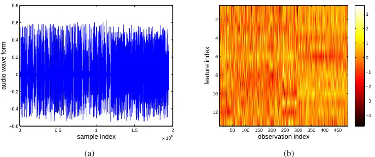
Figure 7: Original audio waveform, (a), and representation in terms of MFCC features, (b).

With the kernel in (2.1)specified in a temporal (one-dimensional) space, the proposed LSBP is naturally extended to segmentation of sequential data, such as for speaker diarization (Ben et al., 2004; Tranter and Reynolds, 2006; Fox et al., 2008). Provided with a spoken document consisting of multiple speakers, speaker diarization is the process of segmenting the audio signal into contiguous temporal regions, and within a given region a particular individual is speaking. Further, one also wishes to group all temporal regions in which a specific individual is speaking.

(17)

to which we compare, is a sticky HMM (Fox et al., 2008), in which the speech is represented by an HMM with Gaussian state-dependent emissions; to associate a given speaker with a particular state, the states are made to be persistent, or “sticky’, with the state-dependent degree of stickiness also inferred.

We consider identification of different speakers from a recording of broadcast news, which may be downloaded with its ground truth.1 The spoken document has a length of 122.05 seconds, and consists of three speakers. Figure 7(a) presents the audio waveform with a sampling rate of 16000 Hz. The ground truth indicates that Speaker 1 talked within the first 13.77 seconds, followed by Speaker 2 until the 59.66 second, then Speaker 1 began to talk again until 74.15 seconds, and Speaker 3 followed and speaks until the end.

0 100 200 300 400 500

1 2 3 4 5 6 7 8 9 10

observation index

cluster index

(a)

0 100 200 300 400 500

1 2 3 4 5 6 7 8 9 10

observation index

cluster index

(b)

0 100 200 300 400 500

1 2 3 4 5 6 7 8 9 10

observation index

cluster index

(c)

0 100 200 300 400 500

1 2 3 4 5 6 7 8 9 10

observation index

cluster index

(d)

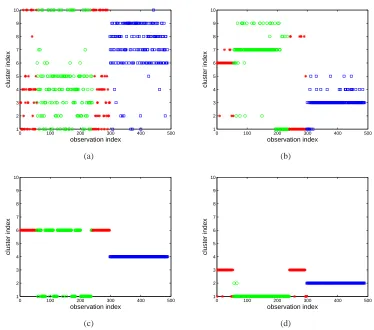
Figure 8: Segmentation results for the audio recording. The colored symbols denote the ground truth: red represents Speaker 1, green represents Speaker 2, blue represents Speaker 3. Each MFCC feature vector is assigned to a cluster index (K=10), with the index shown along the vertical axis. (a) DP, (b) KSBP, (c) sticky HMM using VB inference, (d) LSBP

For the feature vector, we computed the first 13 Mel Frequency Cepstral Coefficients (MFCCs) (Ganchev et al., 2005) over a 30 ms window every 10 ms, and defined the observations as averages over every 250 ms block, without overlap. We used the first 13 MFCCs because the high frequency

(18)

content of these features contained little discriminative information (Fox et al., 2008). The software that we used to extract the MFCCs feature can be downloaded online.2There are 488 feature vectors in total, shown in Figure 7(b); the features are normalized to zero mean and the standard deviation is made equal to one.

To apply the DP, KSBP and LSBP Gaussian mixture models on this data, we set the truncation level as K=10. To calculate the temporal distance between each pair of observations, we take the observation index from 1 to 488 as the location coordinates in (2.1) for s. The potential kernel-width set isΨ∗={50,100, . . . ,1000} for LSBP and KSBP; note that these are the same range of parameters used to present the generative model in Figure 2. The experiment shows that all the models converge after 20 VB iterations.

For the sticky HMM, we employed two distinct forms of posterior computation: (i) a VB anal-ysis, which is consistent with the methods employed for the other models; and (ii) a Gibbs sampler, analogous to that employed in the original sticky-HMM paper (Fox et al., 2008). For both the VB and Gibbs sampler, a truncated stick-breaking representation was used for the DP draws from the hierarchical Dirichlet process (HDP); see Fox et al. (2008) for a discussion of how the HDP is employed in this model.

observation index

o

b

s

e

rv

a

ti

o

n

i

n

d

e

x

sticky iHMM

1 56 240 298 488 1

56

240

298

488 0

0.1 0.2 0.3 0.4 0.5 0.6 0.7 0.8 0.9 1

Speaker 1

Speaker 2

Speaker 1

Speaker 3

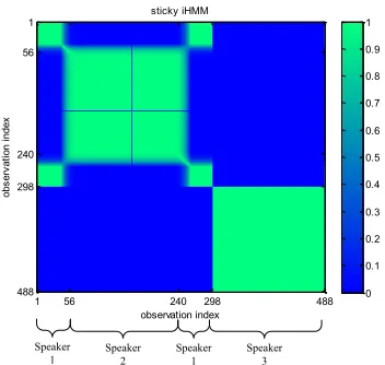
Figure 9: Sticky HMM results for the data in Figure 7(a), based on a Gibbs sampler. The figure denotes the fraction of times within the collection samples that a given portion of the waveform shares the same underlying state.

To segment the audio data, we labeled each observation to the index of the cluster with the largest probability value, and the results are shown in Figure 8 (here the sticky-HMM results were computed via VB analysis). To indicate the ground truth, different symbols and colors are used to represent different speakers.

From the results in Figure 8, the proposed LSBP yields the best segmentation performance, with results in close agreement with ground truth. We found the sticky-HMM results to be very sensitive to VB initialization, and the results in Figure 8 were the best we could achieve.

(19)

While the sticky HMM did not yield reliable VB-computed results, it performed well when a Gibbs sampler was employed (as in the work Fox et al., 2008). In Figure 9 are shown the fraction of times within the collection Gibbs samples that a given portion of the signal share the same un-derlying state; note that the results are in very close agreement with “truth”. We cannot plot the Gibbs results in the same form as the VB results in Figure 8 due to label switching within the Gibbs sampler. The Gibbs-sampler results were computed using 5000 burn iterations and 5000 collection iterations.

These results demonstrate that the proposed LSBP, based on a fast VB solution, yields results commensurate with a state-of-the-art method (the sticky HMM based on a Gibbs sampler). On the same PC, the VB LSBP results required approximately 45 seconds of CPU time, while the Gibbs sticky-HMM results required 3 hours; in both cases the code was written in non-optimized Matlab, and these numbers should be viewed as providing a relative view of computational expense. The accuracy and speed of the VB LSBP is of interest for large-scale problems, like those considered in the next section. Further, the LSBP is a general-purpose algorithm, applicable to time- and spatially-dependent data (images), while the sticky HMM is explicitly designed for time-dependent data.

In the LSBP, DP, and KSBP analyses, we do not set the number of clusters a priori and the models infer the number of clusters automatically from the data. Therefore, we fixed the truncation level to K=10 for all models, and the clustering results are shown in Figure 6, with different colors representing the cluster index (mixture component to which a data sample is assigned).

In Figure 2 we illustrated a draw from the LSBP prior, in the absence of any data. The param-eters of that example (number of samples, the definition of Nc, and the libraryΨ∗) were selected

as to correspond to this audio example. To generate the draws in Figure 2, a spike-and-slab prior was employed, since the Student-t prior would prefer (in the absence of data) to set all coefficients to zero (or near zero), with high probability. Further, for related reasons we treated the bias terms

wk0 distinct from the other coefficients. We now consider a draw from the LSBP posterior, based

on the audio data considered above. This gives further insight into the machinery of the LSBP. We also emphasize that, in this example based on real data, as in all examples shown in this section, we impose sparseness via the Student-t prior. Therefore, when looking at the posterior, we may see which coefficients wkihave been “pulled” away from zero such that the model fits the observed data.

A representative draw from the LSBP posterior is shown in Figure 10, using the same presentation format as applied to the draw from the prior in Figure 2. Note that only three sticks have appreciable probability for any time t, and the segments tend to be localized, with near-unity probability of using a corresponding model parameter within a given segment. While the spike-slab prior was needed to manifest desirable draws from the prior alone, the presence of data simplifies the form of the LSBP prior, based only on a relatively standard use of the hierarchical Student-t construction.

5.3 Image Segmentation with LSBP

The images considered first are from Microsoft Research Cambridge3and each image has 320×213 pixels. To apply the hierarchical model to image segmentation, we first over-segment each im-age into 1,000 “superpixels”, which are local, coherent and preserve most of the structure neces-sary for segmentation at the scale of interest (Ren and Malik, 2003). The software used for this

3. Images can be downloaded from http://research.microsoft.com/en-us/projects/

(20)

0 100 200 300 400 500 −50

0 50

w1

0 100 200 300 400 500

−50 0 50

w2

0 100 200 300 400 500

−50 0 50

w3

0 100 200 300 400 500

−50 0 50 w4 basis location (a)

0 100 200 300 400 500

−50 0 50

g1

(t)

0 100 200 300 400 500

−50 0 50

g2

(t)

0 100 200 300 400 500

−50 0 50

g3

(t)

0 100 200 300 400 500

−50 0 50 g4 (t) t (b)

0 100 200 300 400 500

0 0.5 1 σ [g1 (t)]

0 100 200 300 400 500

0 0.5 1 σ [g2 (t)]

0 100 200 300 400 500

0 0.5 1 σ [g3 (t)]

0 100 200 300 400 500

0 0.5 1 σ [g4 (t)] t (c)

0 100 200 300 400 500

0 0.5 1

π1

(t)

0 100 200 300 400 500

0 0.5 1

π2

(t)

0 100 200 300 400 500

0 0.5 1

π3

(t)

0 100 200 300 400 500

0 0.5 1 π4 (t) t (d)

Figure 10: Example draw from the LSBP posterior, for the audio data under test. (a)wk, (b) gk(t)

, (c)σk(t), (d)πk(t)

is described in Mori (2005), and can be downloaded at http://fas.sfu.ca/˜mori/research/ superpixels/. Each superpixel is represented by both color and texture descriptors, based on the local RGB, hue feature vectors (Weijer and Schmid, 2006), and also the values of Maximum Response (MR) filter banks (Varma and Zisserman, 2002). We discretize these features using a codebook of size 32, and then calculate the distributions (Ahonen and Pietik¨ainen, 2009) for each feature within each superpixel as visual words (Cao and Li, 2007; Wang and Grimson, 2007).

Since each superpixel is represented by three visual words, the mixture componentsθ∗_k are three multinomial distributions as{Mult(p1∗_k)⊗Mult(p2_k∗)⊗Mult(p3∗_k)}for k=1, . . . ,K. The variational

distribution q(θ_k∗) is Dir(p1_k∗|β˜1_k)⊗Dir(p2∗_k|β˜2_k)⊗Dir(p3∗_k|β˜_k3), and within VB inference we opti-mize the parameters ˜β1

k, ˜β2k, and ˜β3k.

To perform segmentation at the patch level (each superpixel corresponds to one patch), the cen-ter of each superpixel is recorded as the location coordinate sn. The discrete kernel-width setΨ∗is

(21)

distance associated with any two data points’ spatial locations within this image. To save computa-tional resources, we chose as basis locations{ˆsi}N_i₌₁c the spatial centers of every tenth superpixel in

a given image, after sequentially indexing the superpixels (we found that if we do not perform this subsampling, very similar segmentation results are achieved, but at greater computational expense).

Three representative example images are shown in Figures 11(a), (b) and (c); the superpixels are generated by over-segmentation (Mori, 2005) on each image, with associated over-segmentation re-sults shown in Figures 11(d), (e) and (f). The segmentation task now reduces to grouping/clustering the superpixels based on the associated image feature vector and associated spatial information. To examine the effect of the truncation level K, we considered K from 2 to 10 and quantified the VB approximation to the model evidence (marginal likelihood). The segmentation performance for each of these images is shown in Figure 11(g), (h) and (i), using respectively K=4, 3 and 6, based on the model evidence (discussed further below). These (typical) results are characterized by homogeneous segments with sharp boundaries. In Figure 11(j), (k) and (l), the segmentation results are shown with K fixed at K=10. In this case the LSBP has ten sticks; however, based on the segmentation there are a subset of sticks (5, 8 and 7, respectively) inferred to have appreciable amplitude.

Based upon these representative example results, which are consistent with a large number of tests on related images, we make the following observations. Considering first the “chimney” results in Figure 11(a), (g) and (j), for example, we note that there are portions of the brick that have textural differences. However, the prior tends to favor contiguous segments, and one solid texture is manifested for the bricks. We also note the sharp boundaries manifested in the segments, despite the fact that the logistic-regression construction is only using simple Gaussian kernels (not particularly optimized for near-linear boundaries). For the relatively simple “chimney” image, the segmentation results are very similar with different initializations of K (Figure 11(g)) and simply truncating the sticks at a “large” value (Figure 11(j) with K=10).

The “cow” example is more complex, pointing out further characteristics of LSBP. We again observe homogeneous contiguous segments with sharp boundaries. In this case a smaller K yields (as expected) a simpler segmentation (Figure 11(h)). All of the relatively dark cows are segmented together. By contrast, with the initialization of K=10, the results in Figure 11(k) capture more details in the cows. However, we also note that in Figure 11(k) the clouds are properly assigned to a distinctive type of segment, while in Figure 11(h) the clouds are just included in the sky clus-ter/segment. Similar observations are also obtained from the “flower” example for Figure 11(c), with more flower texture details kept with a large truncation level setting in Figure 11(l) than the result with a smaller K shown in Figure 11(i).

Because of the sampling of the kernel width, the lower bound of the log model evidence did not increase monotonically in general. For the “chimney” example considered in Figure 11(a), the log model evidence was found to sequentially increase approximately within the first 20 iterations and then converge to the local optimal solution with small fluctuations, as shown in Figure 12(a) with a model of K=4. To test the model performance with different initializations of K, we calculate the mean and standard deviation of the lower bound after 25 iterations when K equals from 2 to 10, as plotted in Figure 12(b); from this figure one clearly observes that the data favor the model with

(22)

(a) (b) (c)

(d) (e) (f)

1 2 3 4

(g)

1 2 3

(h)

1 2 3 4 5 6

(i)

1 2 3 4 5

(j)

1 2 3 4 5 6 7 8

(k)

1 2 3 4 5 6 7

(l)

(23)

0 10 20 30 40 50 60 −8

−7 −6 −5 −4 −3x 10

4

Iteration times

Lowerbound

(a)

2 3 4 5 6 7 8 9 10 −7

−6.5 −6 −5.5 −5 −4.5 −4 −3.5x 10

4

Initialized number of components K

Mean and St.dev. of the lowerbound

(b)

Figure 12: LSBP Segmentation for three image examples. (a)VB iteration lowerbound for image “chimney” with K=4; (b) Approximating the model evidence as a function of K for image “chimney”.

To further evaluate the performance of LSBP for image segmentation, we also consider several other state-of-art methods, including two other non-parametric statistical models: the Dirichlet pro-cess (DP) (Sethuraman, 1994) and the kernel stick-breaking propro-cess (KSBP) (An et al., 2008). We also consider two graph-based spectral decomposition methods: normalized cuts (Ncuts) (Shi and Malik, 2000) and multi-scale Ncut with long-range graph connections (Cour et al., 2005). Further, we consider the Student-t distribution mixture model (Stu.-t MM) (Sfikas et al., 2007), and also spatially varying mixture segmentation with edge preservation (St.-svgm) (Sfikas et al., 2008). We consider the same data source as in the previous examples, but for the next set of results segmen-tation “ground truth” was provided with the data. The data are divided into eight categories: trees, houses, cows, faces, sheep, flowers, lake and street; each category has thirty images. All models were initialized with a segment number of K=10.

Figure 13 shows typical segmentation results for the different algorithms. Given a segment count number, both the normalized cuts and the multi-scale Ncut produced very smooth segmen-tations, while certain textured regions might be split into several pieces. The Student-t distribution mixture model (Stu.-t MM) yields a relatively robust segmentation, but it is sensitive to the texture appearance. Compared with Stu.-t MM, the spatially varying mixtures (St.-svgm) favors a more contiguous segmentation for the texture region, preserving edges; this may make a good tradeoff between keeping coherence and capturing details, but the segmentation performance is degraded by redundant boundaries, such as those within the goose body. Compared with these state-of-art algo-rithms, the LSBP results appear to be very competitive. Among the Bayesian methods (DP, KSBP and LSBP), LSBP tends to yield better segmentation, characterized by homogeneous segmentation regions and sharp segment boundaries.

(24)

original image

ground truth

li d Normalized

cuts

Multi-scale Ncut

Stu.-t MM

St.-svgm

DP

KSBP

LSBP

Figure 13: Segmentation examples of different methods with an initialization of K=10. From top to down, each row shows: the original image, the image ground truth, normalized cuts, multiscale Ncut, Student-t distributions mixture model (Stu.-t MM), spatially varying mixtures (St.-svgm), DP mixture, KSBP mixture, and the LSBP mixture model.

thirty images for each category; the statistics for the two measures are depicted in Tables 1 and 2, considering all 240 images and various K.

Compared with other state-of-the-art methods, the LSBP yields relatively larger mean and me-dian values for average RI, and relatively small average VoI, for most K. For K=2 and 4 the spatially varying mixtures (St.-svgm) shows the largest RI values, while it does not yield similar effectiveness as K increases. In contrast, the LSBP yields a relatively stable RI and VoI from K=4 to 10. This property is more easily observed in Figure 14, which shows the averaged RI and VoI evaluated as a function of K, for categories “houses” and “cows”. The Stu.-t MM, St.-svgm, DP and KSBP have similar performances for most K; LSBP generates a competitive result with a smaller

K, and also yields robust performance with a large K.

We also considered the Berkeley 300 data set.4These images have size 481×321 pixels, and we also over-segmented each image into 1000 superpixels. Both the RI and VoI measures are calculated on average, with the multiple labels (human labeled) provided with the data. Each individual image

4. Data set can be downloaded from http://www.eecs.berkeley.edu/Research/Projects/CS/vision/

(25)

K 2 4 6 8 10

Ncuts

mean 0.5552 0.6169 0.6269 0.6180 0.6093 median 0.5259 0.6098 0.6376 0.6286 0.6235 st. dev. 0.0953 0.1145 0.1317 0.1402 0.1461

Multi-scale Ncuts

Stu.-t MM

St.-svgm

DP

KSBP

LSBP

mean 0.6516 0.6791 0.6804 0.6704 0.6777

median 0.6384 0.6921 0.6900 0.6835 0.6885

st. dev. 0.1310 0.1202 0.1263 0.1294 0.1319

Table 1: Statistics on the averaged Rand Index (RI) over 240 images as a function of K (Microsoft Research Cambridge images).

typically has roughly ten segments within the ground truth. We calculated the evaluation measures for K=5, 10 and 15. Table 3 presents results, demonstrating that all methods produced competitive results for both the RI and VoI measures. By a visual evaluation of the segmentation results (see Figure 15), multi-scale Ncut is not as good as the other methods when the segments are of irregular shape and unequal size.

The purpose of this section was to demonstrate that LSBP yields competitive segmentation performance, compared with many state-of-the-art algorithms. It should be emphasized that there is no perfect way of quantifying segmentation performance, especially since the underlying “truth” is itself subjective. An important advantage of the Bayesian methods (DP, KSBP and LSBP) is that they may be readily extended to joint segmentation of multiple images, considered in the next section.

5.4 Joint Image Segmentation with H-LSBP