DirectLiNGAM: A Direct Method for Learning a Linear
Non-Gaussian Structural Equation Model
Shohei Shimizu [email protected]
Takanori Inazumi [email protected]
Yasuhiro Sogawa [email protected]
The Institute of Scientific and Industrial Research Osaka University
Mihogaoka 8-1, Ibaraki, Osaka 567-0047, Japan
Aapo Hyv¨arinen [email protected]
Department of Computer Science and Department of Mathematics and Statistics University of Helsinki
Helsinki Institute for Information Technology FIN-00014, Finland
Yoshinobu Kawahara [email protected]
Takashi Washio [email protected]
The Institute of Scientific and Industrial Research Osaka University
Mihogaoka 8-1, Ibaraki, Osaka 567-0047, Japan
Patrik O. Hoyer [email protected]
Helsinki Institute for Information Technology University of Helsinki
FIN-00014, Finland
Kenneth Bollen [email protected]
Department of Sociology, CB 3210 Hamilton Hall University of North Carolina
Chapel Hill, NC 27599-3210 U.S.A.
Abstract
Structural equation models and Bayesian networks have been widely used to analyze causal rela-tions between continuous variables. In such frameworks, linear acyclic models are typically used to model the data-generating process of variables. Recently, it was shown that use of non-Gaussianity identifies the full structure of a linear acyclic model, that is, a causal ordering of variables and their connection strengths, without using any prior knowledge on the network structure, which is not the case with conventional methods. However, existing estimation methods are based on iterative search algorithms and may not converge to a correct solution in a finite number of steps. In this pa-per, we propose a new direct method to estimate a causal ordering and connection strengths based on non-Gaussianity. In contrast to the previous methods, our algorithm requires no algorithmic parameters and is guaranteed to converge to the right solution within a small fixed number of steps if the data strictly follows the model, that is, if all the model assumptions are met and the sample size is infinite.
1. Introduction
Many empirical sciences aim to discover and understand causal mechanisms underlying various natural phenomena and human social behavior. An effective way to study causal relationships is to conduct a controlled experiment. However, performing controlled experiments is often ethically impossible or too expensive in many fields including social sciences (Bollen, 1989), bioinformatics (Rhein and Strimmer, 2007) and neuroinformatics (Londei et al., 2006). Thus, it is necessary and important to develop methods for causal inference based on the data that do not come from such controlled experiments.
Structural equation models (SEM) (Bollen, 1989) and Bayesian networks (BN) (Pearl, 2000; Spirtes et al., 1993) are widely applied to analyze causal relationships in many empirical studies. A linear acyclic model that is a special case of SEM and BN is typically used to analyze causal effects between continuous variables. Estimation of the model commonly uses only the covariance structure of the data and in most cases cannot identify the full structure, that is, a causal ordering and connection strengths, of the model with no prior knowledge on the structure (Pearl, 2000; Spirtes et al., 1993).
In Shimizu et al. (2006), a non-Gaussian variant of SEM and BN called a linear non-Gaussian acyclic model (LiNGAM) was proposed, and its full structure was shown to be identifiable without pre-specifying a causal order of the variables. This feature is a significant advantage over the con-ventional methods (Spirtes et al., 1993; Pearl, 2000). A non-Gaussian method to estimate the new model was also developed in Shimizu et al. (2006) and is closely related to independent component analysis (ICA) (Hyv¨arinen et al., 2001). In the subsequent studies, the non-Gaussian framework has been extended in various directions for learning a wider variety of SEM and BN (Hoyer et al., 2009; Hyv¨arinen et al., 2010; Lacerda et al., 2008). In what follows, we refer to the non-Gaussian model as LiNGAM and the estimation method as ICA-LiNGAM algorithm.
Most of major ICA algorithms including Amari (1998) and Hyv¨arinen (1999) are iterative search methods (Hyv¨arinen et al., 2001). Therefore, the ICA-LiNGAM algorithms based on the ICA algo-rithms need some additional information including initial guess and convergence criteria. Gradient-based methods (Amari, 1998) further need step sizes. However, such algorithmic parameters are hard to optimize in a systematic way. Thus, the ICA-based algorithms may get stuck in local optima and may not converge to a reasonable solution if the initial guess is badly chosen (Himberg et al., 2004).
The paper is structured as follows. First, in Section 2, we briefly review LiNGAM and the ICA-based LiNGAM algorithm. We then in Section 3 introduce a new direct method. The performance of the new method is examined by experiments on artificial data in Section 4, and experiments on real-world data in Section 5. Conclusions are given in Section 6. Preliminary results were presented in Shimizu et al. (2009), Inazumi et al. (2010) and Sogawa et al. (2010).
2. Background
In this section, we first review LiNGAM and the ICA-LiNGAM algorithm (Shimizu et al., 2006) in Sections 2.1-2.3 and next mention potential problems of the ICA-based algorithm in Section 2.4.
2.1 A Linear Non-Gaussian Acyclic Model: LiNGAM
In Shimizu et al. (2006), a non-Gaussian variant of SEM and BN, which is called LiNGAM, was proposed. Assume that observed data are generated from a process represented graphically by a directed acyclic graph, that is, DAG. Let us represent this DAG by a m×m adjacency matrix B={bi j}where every bi j represents the connection strength from a variable xj to another xi in the
DAG. Moreover, let us denote by k(i) a causal order of variables xi in the DAG so that no later
variable determines or has a directed path on any earlier variable. (A directed path from xito xj is a
sequence of directed edges such that xj is reachable from xi.) We further assume that the relations
between variables are linear. Without loss of generality, each observed variable xi is assumed to
have zero mean. Then we have
xi=
∑
k(j)<k(i)
bi jxj+ei, (1)
where eiis an external influence. All external influences eiare continuous random variables having
non-Gaussian distributions with zero means and non-zero variances, and eiare independent of each
other so that there are no latent confounding variables (Spirtes et al., 1993). We rewrite the model (1) in a matrix form as follows:
x=Bx+e, (2)
where x is a p-dimensional random vector, and B could be permuted by simultaneous equal row and column permutations to be strictly lower triangular due to the acyclicity assumption (Bollen, 1989). Strict lower triangularity is here defined as a lower triangular structure with all zeros on the diagonal. Our goal is to estimate the adjacency matrix B by observing data x only. Note that we do not assume that the distribution of x is faithful (Spirtes et al., 1993) to the generating graph.
We note that each bi j represents the direct causal effect of xj on xi and each ai j, the (i,j)-th
element of the matrix A=(I−B)−1, the total causal effect of x
j on xi(Hoyer et al., 2008).
We emphasize that xiis equal to eiif no other observed variable xj ( j6=i) inside the model has
a directed edge to xi, that is, all the bi j ( j6=i) are zeros. In such a case, an external influence ei is
observed as xi. Such an xiis called an exogenous observed variable. Otherwise, eiis called an error.
For example, consider the model defined by
x2 = e2,
x1 = 1.5x2+e1,
where x2 is equal to e2 since it is not determined by either x1 or x3. Thus, x2 is an exogenous observed variable, and e1and e3are errors. Note that there exists at least one exogenous observed
variable xi(=ei) due to the acyclicity and the assumption of no latent confounders.
An exogenous observed variable is usually defined as an observed variable that is determined outside of the model (Bollen, 1989). In other words, an exogenous observed variable is a variable that any other observed variable inside the model does not have a directed edge to. The definition does not require that it is equal to an independent external influence, and the external influences of exogenous observed variables may be dependent. However, in the LiNGAM (2), an exogenous observed variable is always equal to an independent external influence due to the assumption of no latent confounders.
2.2 Identifiability of the Model
We next explain how the connection strengths of the LiNGAM (2) can be identified as shown in Shimizu et al. (2006). Let us first solve Equation (2) for x. Then we obtain
x=Ae, (3)
where A= (I−B)−1 is a mixing matrix whose elements are called mixing coefficients and can be permuted to be lower triangular as well due to the aforementioned feature of B and the nature of matrix inversion. Since the components of e are independent and non-Gaussian, Equation (3) defines the independent component analysis (ICA) model (Hyv¨arinen et al., 2001), which is known to be identifiable (Comon, 1994; Eriksson and Koivunen, 2004).
ICA essentially can estimate A (and W=A−1=I−B), but has permutation, scaling and sign indeterminacies. ICA actually gives WICA=PDW, where P is an unknown permutation matrix, and
D is an unknown diagonal matrix. But in LiNGAM, the correct permutation matrix P can be found (Shimizu et al., 2006): the correct P is the only one that gives no zeros in the diagonal of DW since B should be a matrix that can be permuted to be strictly lower triangular and W=I−B. Further, one can find the correct scaling and signs of the independent components by using the unity on the diagonal of W=I−B. One only has to divide the rows of DW by its corresponding diagonal elements to obtain W. Finally, one can compute the connection strength matrix B=I−W.
2.3 ICA-LiNGAM Algorithm
The ICA-LiNGAM algorithm presented in Shimizu et al. (2006) is described as follows:
ICA-LiNGAM algorithm
1. Given a p-dimensional random vectorxand its p×nobserved data matrixX, apply an ICA algorithm (FastICA of Hyv ¨arinen 1999 using hyperbolic tangent function) to obtain an estimate ofA.
2. Find the unique permutation of rows ofW=A−1which yields a matrixfWwithout any zeros on the main diagonal. The permutation is sought by minimizing∑i1/|fWii|.
4. Compute an estimateBbofBusingBb=I−fW′.
5. Finally, to estimate a causal orderk(i), find the permutation matrix ePof Bb yielding a matrix e
B=PeBbPeT which is as close as possible to a strictly lower triangular structure. The lower-triangularity ofBe can be measured using the sum of squared bi j in its upper triangular part
∑i≤jeb2i j for small number of variables, say less than 8. For higher-dimensional data, the
fol-lowing approximate algorithm is used, which sets small absolute valued elements inBeto zero and tests if the resulting matrix is possible to be permuted to be strictly lower triangular:
(a) Set thep(p+1)/2smallest (in absolute value) elements ofBbto zero. (b) Repeat
i. Test ifBbcan be permuted to be strictly lower triangular. If the answer is yes, stop and return the permutedBb, that is,eB.
ii. Additionally set the next smallest (in absolute value) element ofBbto zero.
2.4 Potential Problems of ICA-LiNGAM
The original ICA-LiNGAM algorithm has several potential problems: i) Most ICA algorithms in-cluding FastICA (Hyv¨arinen, 1999) and gradient-based algorithms (Amari, 1998) may not converge to a correct solution in a finite number of steps if the initially guessed state is badly chosen (Himberg et al., 2004) or if the step size is not suitably selected for those gradient-based methods. The appro-priate selection of such algorithmic parameters is not easy. In contrast, our algorithm proposed in the next section is guaranteed to converge to the right solution in a fixed number of steps equal to the number of variables if the data strictly follows the model. ii) The permutation algorithms in Steps 2 and 5 are not scale-invariant. Hence they could give a different or even wrong ordering of variables depending on scales or standard deviations of variables especially when they have a wide range of scales. However, scales are essentially not relevant to the ordering of variables. Though such bias would vanish for large enough sample sizes, for practical sample sizes, an estimated ordering could be affected when variables are normalized to make unit variance for example, and hence the estimation of a causal ordering becomes quite difficult.
3. A Direct Method: DirectLiNGAM
In this section, we present a new direct estimation algorithm named DirectLiNGAM.
3.1 Identification of an Exogenous Variable Based on Non-Gaussianity and Independence In this subsection, we present two lemmas and a corollary1that ensure the validity of our algorithm proposed in the next subsection 3.2. The basic idea of our method is as follows. We first find an exogenous variable based on its independence of the residuals of a number of pairwise regressions (Lemma 1). Next, we remove the effect of the exogenous variable from the other variables using least squares regression. Then, we show that a LiNGAM also holds for the residuals (Lemma 2) and that the same ordering of the residuals is a causal ordering for the original observed variables as
well (Corollary 1). Therefore, we can find the second variable in the causal ordering of the original observed variables by analyzing the residuals and their LiNGAM, that is, by applying Lemma 1 to the residuals and finding an “exogenous” residual. The iteration of these effect removal and causal ordering estimates the causal order of the original variables.
We first quote Darmois-Skitovitch theorem (Darmois, 1953; Skitovitch, 1953) since it is used to prove Lemma 1:
Theorem 1 (Darmois-Skitovitch theorem) Define two random variables y1and y2as linear
com-binations of independent random variables si(i=1,· · ·, q):
y1=
q
∑
i=1
αisi, y2=
q
∑
i=1 βisi.
Then, if y1and y2are independent, all variables sjfor whichαjβj6=0 are Gaussian.
In other words, this theorem means that if there exists a non-Gaussian sjfor whichαjβj6=0, y1and
y2are dependent.
Lemma 1 Assume that the input data x strictly follows the LiNGAM (2), that is, all the model assumptions are met and the sample size is infinite. Denote by ri(j)the residual when xiis regressed
on xj: r(ij)=xi−covvar(x(ix,xj)
j) xj (i6= j). Then a variable xjis exogenous if and only if xjis independent of its residuals ri(j)for all i6= j.
Proof (i) Assume that xj is exogenous, that is, xj=ej. Due to the model assumption and
Equa-tion (3), one can write xi=ai jxj+e¯i(j)(i6=j), where ¯ei(j)=∑h6=jaiheh and xj are independent, and ai j
is a mixing coefficient from xj to xiin Equation (3). The mixing coefficient ai j is equal to the
re-gression coefficient when xi is regressed on xj since cov(xi,xj)=ai jvar(xj). Thus, the residual ri(j)
is equal to the corresponding error term, that is, r(ij)=e¯i(j). This implies that xj and ri(j)(=e¯
(j)
i )are
independent.
(ii) Assume that xj is not exogenous, that is, xj has at least one parent. Let Pj denote the
(non-empty) set of the variable subscripts of parent variables of xj. Then one can write xj=∑h∈Pjbjhxh+ ej, where xhand ej are independent and each bjhis non-zero. Let a vector xPj and a column vector bPj collect all the variables in Pj and the corresponding connection strengths, respectively. Then, the covariances between xPj and xj are
E(xPjxj) = E{xPj(b
T
PjxPj+ej)}
= E(xPjb
T
PjxPj) +E(xPjej)
= E(xPjx
T
Pj)bPj. (4)
The covariance matrix E(xPjx
T
Pj)is positive definite since the external influences ehthat correspond to those parent variables xh in Pj are mutually independent and have positive variances. Thus, the
covariance vector E(xPjxj) =E(xPjx
T
a variable xi(i∈Pj) that cov(xi,xj)6=0, we have
r(ij) = xi−
cov(xi,xj)
var(xj)
xj
= xi−
cov(xi,xj)
var(xj) h
∑
∈Pj
bjhxh+ej
!
=
1−bjicov(xi,xj) var(xj)
xi−
cov(xi,xj)
var(xj) h∈P
∑
j,h6=i bjhxh
−cov(xi,xj) var(xj)
ej.
Each of those parent variables xh (including xi) in Pj is a linear combination of external influences
other than ej due to the relation of xhto ejthat xj=∑h∈Pjbjhxh+ej=∑h∈Pjbjh ∑k(t)≤k(h)ahtet
+
ej , where et and ej are independent. Thus, the ri(j)and xj can be rewritten as linear combinations
of independent external influences as follows:
r(ij) =
1−bjicov(xi,xj) var(xj) l
∑
6=jailel
!
−cov(xi,xj) var(xj) h∈P
∑
j,h6=ibjh
∑
t6=jahtet
!
−cov(xi,xj) var(xj)
ej, (5)
xj =
∑
h∈Pj
bjh
∑
t6=jahtet
!
+ej. (6)
The first two terms of Equation (5) and the first term of Equation (6) are linear combinations of external influences other than ej, and the third term of Equation (5) and the second term of
Equa-tion (6) depend only on ej and do not depend on the other external influences. Further, all the
external influences including ej are mutually independent, and the coefficient of non-Gaussian ej
on ri(j)and that on xj are non-zero. These imply that ri(j)and xj are dependent since ri(j), xjand ej
correspond to y1, y2, sj in Darmois-Skitovitch theorem, respectively.
From (i) and (ii), the lemma is proven.
Lemma 2 Assume that the input data x strictly follows the LiNGAM (2). Further, assume that a variable xj is exogenous. Denote by r(j)a (p-1)-dimensional vector that collects the residuals ri(j)
when all xi of x are regressed on xj (i6=j). Then a LiNGAM holds for the residual vector r(j):
r(j)=B(j)r(j)+e(j), where B(j)is a matrix that can be permuted to be strictly lower-triangular by a simultaneous row and column permutation, and elements of e(j)are non-Gaussian and mutually independent.
Proof Without loss of generality, assume that B in the LiNGAM (2) is already permuted to be strictly lower triangular and that xj=x1. Note that A in Equation (3) is also lower triangular (al-though its diagonal elements are all ones). Since x1 is exogenous, ai1 are equal to the regression
by least squares estimation, one gets the first column of A to be a zero vector, and x1does not affect the residuals r(i1). Thus, we again obtain a lower triangular mixing matrix A(1)with all ones in the diagonal for the residual vector r(1)and hence have a LiNGAM for the vector r(1).
Corollary 1 Assume that the input data x strictly follows the LiNGAM (2). Further, assume that a variable xjis exogenous. Denote by kr(j)(i)a causal order of r(ij). Recall that k(i)denotes a causal
order of xi. Then, the same ordering of the residuals is a causal ordering for the original observed
variables as well: kr(j)(l)<kr(j)(m)⇔k(l)<k(m).
Proof As shown in the proof of Lemma 2, when the effect of an exogenous variable x1is removed from the other observed variables, the second to p-th columns of A remain the same, and the sub-matrix of A formed by deleting the first row and the first column is still lower triangular. This shows that the ordering of the other variables is not changed and proves the corollary.
Lemma 2 indicates that the LiNGAM for the (p−1)-dimensional residual vector r(j) can be handled as a new input model, and Lemma 1 can be further applied to the model to estimate the next exogenous variable (the next exogenous residual in fact). This process can be repeated until all variables are ordered, and the resulting order of the variable subscripts shows the causal order of the original observed variables according to Corollary 1.
To apply Lemma 1 in practice, we need to use a measure of independence which is not restricted to uncorrelatedness since least squares regression gives residuals always uncorrelated with but not necessarily independent of explanatory variables. A common independence measure between two variables y1and y2is their mutual information MI(y1,y2)(Hyv¨arinen et al., 2001). In Bach and Jor-dan (2002), a nonparametric estimator of mutual information was developed using kernel methods.2 Let K1and K2represent the Gram matrices whose elements are Gaussian kernel values of the sets of
n observations of y1and y2, respectively. The Gaussian kernel values K1(y(1i),y1(j))and K2(y2(i),y(2j)) (i,j=1,· · ·,n)are computed by
K1(y(1i),y(1j)) = exp
− 1 2σ2ky
(i)
1 −y
(j)
1 k 2
,
K2(y(2i),y
(j)
2 ) = exp
− 1 2σ2ky
(i)
2 −y
(j)
2 k 2
,
where σ>0 is the bandwidth of Gaussian kernel. Further let κdenote a small positive constant. Then, in Bach and Jordan (2002), the kernel-based estimator of mutual information is defined as:
c
MIkernel(y1,y2) =−
1 2log
det
K
κdet
D
κ,where
K
κ ="
K1+n2κI 2
K1K2
K2K1 K2+n2κI 2
#
,
D
κ ="
K1+n2κI 2
0 0 K2+n2κI
2 #
.
As the bandwidthσof Gaussian kernel tends to zero, the population counterpart of the estimator converges to the mutual information up to second order when it is expanded around distributions with two variables y1 and y2 being independent (Bach and Jordan, 2002). The determinants of the Gram matrices K1and K2can be efficiently computed by using the incomplete Cholesky decompo-sition to find their low-rank approximations of rank M (≪ n). In Bach and Jordan (2002), it was suggested that the positive constantκand the width of the Gaussian kernelσare set toκ=2×10⁻³, σ=1/2 for n>1000 andκ=2×10⁻²,σ=1 for n≤1000 due to some theoretical and computa-tional considerations.
In this paper, we use the kernel-based independence measure. We first evaluate pairwise in-dependence between a variable and each of the residuals and next take the sum of the pairwise measures over the residuals. Let us denote by U the set of the subscripts of variables xi, that is,
U={1, · · ·, p}. We use the following statistic to evaluate independence between a variable xj and
its residuals ri(j)=xi−covvar(x(ix,jx)j)xjwhen xiis regressed on xj:
Tkernel(xj;U) =
∑
i∈U,i6=j
c
MIkernel(xj,ri(j)). (7)
Many other nonparametric independence measures (Gretton et al., 2005; Kraskov et al., 2004) and more computationally simple measures that use a single nonlinear correlation (Hyv¨arinen, 1998) have also been proposed. Any such proposed method of independence could potentially be used instead of the kernel-based measure in Equation (7).
3.2 DirectLiNGAM Algorithm
We now propose a new direct algorithm called DirectLiNGAM to estimate a causal ordering and the connection strengths in the LiNGAM (2):
DirectLiNGAM algorithm
1. Given a p-dimensional random vector x, a set of its variable subscriptsU and a p×ndata matrix of the random vector asX, initialize an ordered list of variablesK :=/0andm :=1. 2. Repeat until p−1subscripts are appended toK:
(a) Perform least squares regressions ofxi on xj for alli∈U\K (i6= j) and compute the
residual vectors r(j) and the residual data matrix R(j) from the data matrix X for all
j∈U\K. Find a variablexmthat is most independent of its residuals:
xm=arg min
j∈U\KTkernel(xj;U\K),
whereTkernel is the independence measure defined in Equation (7).
(b) Appendmto the end ofK.
(c) Letx :=r(m),X :=R(m).
4. Construct a strictly lower triangular matrix B by following the order in K, and estimate the connection strengthsbi j by using some conventional covariance-based regression such as
least squares and maximum likelihood approaches on the original random vectorx and the original data matrixX. We use least squares regression in this paper.
3.3 Computational Complexity
Here, we consider the computational complexity of DirectLiNGAM compared with the ICA-LiNGAM with respect to sample size n and number of variables p. A dominant part of Di-rectLiNGAM is to compute Equation (7) for each xj in Step 2(a). Since it requires O(np2M2+
p3M3)operations (Bach and Jordan, 2002) in p−1 iterations, complexity of the step is O(np3M2+
p4M3), where M (≪ n) is the maximal rank found by the low-rank decomposition used in the kernel-based independence measure. Another dominant part is the regression to estimate the matrix B in Step 4. The complexity of many representative regressions including the least square algorithm is O(np3). Hence, we have a total budget of O(np3M2+p4M3). Meanwhile, the ICA-LiNGAM re-quires O(p4)time to find a causal order in Step 5. Complexity of an iteration in FastICA procedure at Step 1 is known to be O(np2). Assuming a constant number C of the iterations in FastICA steps, the complexity of the ICA-LiNGAM is considered to be O(Cnp2+p4). Though general evaluation of the required iteration number C is difficult, it can be conjectured to grow linearly with regards to p. Hence the complexity of the ICA-LiNGAM is presumed to be O(np3+p4).
Thus, the computational cost of DirectLiNGAM would be larger than that of ICA-LiNGAM especially when the low-rank approximation of the Gram matrices is not so efficient, that is, M is large. However, we note the fact that DirectLiNGAM has guaranteed convergence in a fixed number of steps and is of known complexity, whereas for typical ICA algorithms including FastICA, the run-time complexity and the very convergence are not guaranteed.
3.4 Use of Prior Knowledge
Although DirectLiNGAM requires no prior knowledge on the structure, more efficient learning can be achieved if some prior knowledge on a part of the structure is available because then the number of causal orders and connection strengths to be estimated gets smaller.
We present three lemmas to use prior knowledge in DirectLiNGAM. Let us first define a matrix Aknw=[aknwji ]that collects prior knowledge under the LiNGAM (2) as follows:
aknwji :=
0 if xidoes not have a directed path to xj
1 if xihas a directed path to xj
−1 if no prior knowledge is available to know if either of the two cases above(0 or 1)is true.
Due to the definition of exogenous variables and that of prior knowledge matrix Aknw, we readily obtain the following three lemmas.
Lemma 3 Assume that the input data x strictly follows the LiNGAM (2). An observed variable xj
is exogenous if aknwji is zero for all i6=j.
Lemma 4 Assume that the input data x strictly follows the LiNGAM (2). An observed variable xj
Lemma 5 Assume that the input data x strictly follows the LiNGAM (2). An observed variable xj
does not receive the effect of xiif aknwji is zero.
The principle of making DirectLiNGAM algorithm more accurate and faster based on prior knowledge is as follows. We first find an exogenous variable by applying Lemma 3 instead of Lemma 1 if an exogenous variable is identified based on prior knowledge. Then we do not have to evaluate independence between any observed variable and its residuals. If no exogenous variable is identified based on prior knowledge, we next find endogenous (non-exogenous) variables by applying Lemma 4. Since endogenous variables are never exogenous we can narrow down the search space to find an exogenous variable based on Lemma 1. We can further skip to compute the residual of an observed variable and take the variable itself as the residual if its regressor does not receive the effect of the variable due to Lemma 5. Thus, we can decrease the number of causal orders and connection strengths to be estimated, and it improves the accuracy and computational time. The principle can also be used to further analyze the residuals and find the next exogenous residual because of Corollary 1. To implement these ideas, we only have to replace Step 2a in DirectLiNGAM algorithm by the following steps:
2a-1 Find such a variable(s) xj (j∈U\K) that the j-th row of Aknwhas zero in the i-th column
for alli∈U\K (i6= j) and denote the set of such variables byUexo. IfUexo is not empty, set
Uc:=Uexo. IfUexois empty, find such a variable(s)xj(j∈U\K) that the j-th row ofAknwhas
unity in thei-th column for at least one ofi∈U\K(i6= j), denote the set of such variables by
Uend and setUc:=U\K\Uend.
2a-2 Denote byV(j)a set of such a variable subscripti∈U\K (i6= j) thataknwi j =0for all j∈Uc.
First setr(ij):=xi for alli∈V(j), next perform least squares regressions of xi on xj for all
i∈U\K\V(j)(i6= j) and estimate the residual vectorsr(j)and the residual data matrixR(j) from the data matrixX for all j∈Uc. IfUc has a single variable, set the variable to bexm.
Otherwise, find a variablexminUc that is most independent of the residuals:
xm=arg min j∈Uc
Tkernel(xj;U\K),
whereTkernel is the independence measure defined in Equation (7).
4. Simulations
We first randomly generated 5 data sets based on sparse networks under each combination of number of variables p and sample size n (p=10, 20, 50, 100; n=500, 1000, 2000):
1. We constructed the p×p adjacency matrix with all zeros and replaced every element in the lower-triangular part by independent realizations of Bernoulli random variables with success probability s similarly to Kalisch and B¨uhlmann (2007). The probability s determines the sparseness of the model. The expected number of adjacent variables of each variable is given by s(p−1). We randomly set the sparseness s so that the number of adjacent variables was 2 or 5 (Kalisch and B¨uhlmann, 2007).
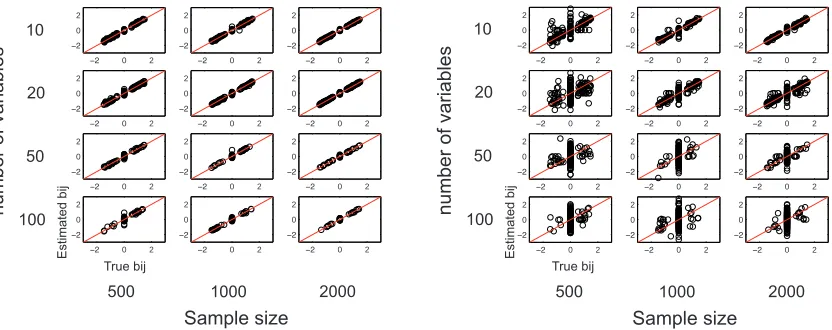
0 2 0 2 0 2 0 2 0 2 0 2 0 2 0 2 0 2 0 2 0 2 0 2 0 2 0 2 0 2 0 2 0 2 0 2 0 2 0 2 0 2 0 2 0 2 0 2 True bij Estimated bij
500 1000 2000 Sample size
number of variables
10 20 50 100 0 2 0 2 0 2 0 2 0 2 0 2 0 2 0 2 0 2 0 2 0 2 0 2 0 2 0 2 0 2 0 2 0 2 0 2 0 2 0 2 0 2 0 2 0 2 0 2 True bij Estimated bij
500 1000 2000 Sample size
number of variables
10
20
50
100
Figure 1: Left: Scatterplots of the estimated bi jby DirectLiNGAM versus the true values for sparse
networks. Right: Scatterplots of the estimated bi jby ICA-LiNGAM versus the true values
for sparse networks.
ei from the interval[1,3]as in Silva et al. (2006). We used the resulting matrix as the
data-generating adjacency matrix B.
3. We generated data with sample size n by independently drawing the external influence vari-ables eifrom various 18 non-Gaussian distributions used in Bach and Jordan (2002) including
(a) Student with 3 degrees of freedom; (b) double exponential; (c) uniform; (d) Student with 5 degrees of freedom; (e) exponential; (f) mixture of two double exponentials; (g)-(h)-(i) symmetric mixtures of two Gaussians: multimodal, transitional and unimodal; (j)-(k)-(l) non-symmetric mixtures of two Gaussians, multimodal, transitional and unimodal; (m)-(n)-(o) symmetric mixtures of four Gaussians: multimodal, transitional and unimodal; (p)-(q)-(r) nonsymmetric mixtures of four Gaussians: multimodal, transitional and unimodal. See Fig-ure 5 of Bach and Jordan (2002) for the shapes of the probability density functions.
4. The values of the observed variables xiwere generated according to the LiNGAM (2). Finally,
we randomly permuted the order of xi.
Further we similarly generated 5 data sets based on dense (full) networks, that is, full DAGs with ev-ery pair of variables is connected by a directed edge, under each combination of number of variables p and sample size n. Then we tested DirectLiNGAM and ICA-LiNGAM on the data sets generated by sparse networks or dense (full) networks. For ICA-LiNGAM, the maximum number of iterations was taken as 1000 (Shimizu et al., 2006). The experiments were conducted on a standard PC using Matlab 7.9. Matlab implementations of the two methods are available on the web:
DirectLiNGAM:http://www.ar.sanken.osaka-u.ac.jp/˜inazumi/dlingam.html, ICA-LiNGAM:http://www.cs.helsinki.fi/group/neuroinf/lingam/.
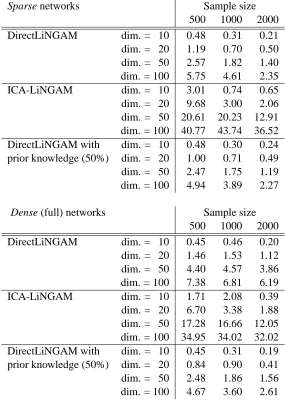
We computed the distance between the true B and ones estimated by DirectLiNGAM and ICA-LiNGAM using the Frobenius norm defined as
q
Sparse networks Sample size
500 1000 2000
DirectLiNGAM dim. = 10 0.48 0.31 0.21
dim. = 20 1.19 0.70 0.50
dim. = 50 2.57 1.82 1.40
dim. = 100 5.75 4.61 2.35
ICA-LiNGAM dim. = 10 3.01 0.74 0.65
dim. = 20 9.68 3.00 2.06
dim. = 50 20.61 20.23 12.91 dim. = 100 40.77 43.74 36.52
DirectLiNGAM with dim. = 10 0.48 0.30 0.24
prior knowledge (50%) dim. = 20 1.00 0.71 0.49
dim. = 50 2.47 1.75 1.19
dim. = 100 4.94 3.89 2.27
Dense (full) networks Sample size
500 1000 2000
DirectLiNGAM dim. = 10 0.45 0.46 0.20
dim. = 20 1.46 1.53 1.12
dim. = 50 4.40 4.57 3.86
dim. = 100 7.38 6.81 6.19
ICA-LiNGAM dim. = 10 1.71 2.08 0.39
dim. = 20 6.70 3.38 1.88
dim. = 50 17.28 16.66 12.05 dim. = 100 34.95 34.02 32.02
DirectLiNGAM with dim. = 10 0.45 0.31 0.19
prior knowledge (50%) dim. = 20 0.84 0.90 0.41
dim. = 50 2.48 1.86 1.56
dim. = 100 4.67 3.60 2.61
Table 1: Median distances (Frobenius norms) between true B and estimated B of DirectLiNGAM and ICA-LiNGAM with five replications.
Tables 1 and 2 show the median distances (Frobenius norms) and median computational times (CPU times), respectively. In Table 1, DirectLiNGAM was better in distances of B and gave more accurate estimates of B than ICA-LiNGAM for all of the conditions. In Table 2, the computation amount of DirectLiNGAM was rather larger than ICA-LiNGAM when the sample size was increased. A main bottleneck of computation was the kernel-based independence measure. However, its computation amount can be considered to be still tractable. In fact, the actual elapsed times were approximately one-quarter of their CPU times respectively probably because the CPU had four cores. Interestingly, the CPU time of ICA-LiNGAM actually decreased with increased sample size in some cases. This is presumably due to better convergence properties.
Sparse networks Sample size
500 1000 2000
DirectLiNGAM dim. = 10 15.16 sec. 37.21 sec. 66.75 sec. dim. = 20 1.56min. 5.75min. 17.22min. dim. = 50 16.25min. 1.34 hrs. 2.70 hrs. dim. = 100 2.35 hrs. 21.17 hrs. 19.90 hrs.
ICA-LiNGAM dim. = 10 0.73 sec. 0.41 sec. 0.28 sec.
dim. = 20 5.40 sec. 2.45 sec. 1.14 sec. dim. = 50 14.49 sec. 21.47 sec. 32.03 sec. dim. = 100 46.32 sec. 58.02 sec. 1.16min. DirectLiNGAM with dim. = 10 4.13 sec. 17.75 sec. 30.95 sec. prior knowledge (50%) dim. = 20 28.02 sec. 1.64min. 4.98min. dim. = 50 7.62min. 28.89min. 1.09 hrs. dim. = 100 48.28min. 1.84 hrs. 7.51 hrs.
Dense (full) networks Sample size
500 1000 2000
DirectLiNGAM dim. = 10 8.05 sec. 24.52 sec. 49.44 sec. dim. = 20 1.00min. 4.23min. 6.91min. dim. = 50 16.18min. 1.12 hrs. 1.92 hrs. dim. = 100 2.16 hrs. 8.59 hrs. 17.24 hrs.
ICA-LiNGAM dim. = 10 0.97 sec. 0.34 sec. 0.27 sec.
dim. = 20 5.35 sec. 1.25 sec. 4.07 sec. dim. = 50 15.58 sec. 21.01 sec. 31.57 sec. dim. = 100 47.60 sec. 56.57 sec. 1.36min. DirectLiNGAM with dim. = 10 2.67 sec. 5.66 sec. 12.31 sec. prior knowledge (50%) dim. = 20 5.02 sec. 31.70 sec. 38.35 sec. dim. = 50 46.74 sec. 2.89min. 5.00min. dim. = 100 3.19min. 10.44min. 19.80min.
Table 2: Median computational times (CPU times) of DirectLiNGAM and ICA-LiNGAM with five replications.
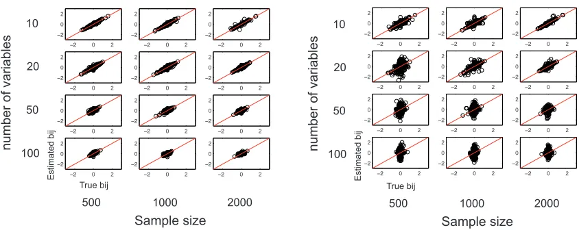
dense (full) networks, respectively. The different plots correspond to different numbers of variables and different sample sizes, where each plot combines the data for different adjacency matrices B and 18 different distributions of the external influences p(ei). We can see that DirectLiNGAM worked
well and better than ICA-LiNGAM, as evidenced by the grouping of the data points onto the main diagonal.
0 2 0 2 0 2 0 2 0 2 0 2 0 2 0 2 0 2 0 2 0 2 0 2 0 2 0 2 0 2 0 2 0 2 0 2 0 2 0 2 0 2 0 2 0 2 0 2 True bij Estimated bij
500 1000 2000 Sample size
number of variables
10 20 50 100 0 2 0 2 0 2 0 2 0 2 0 2 0 2 0 2 0 2 0 2 0 2 0 2 0 2 0 2 0 2 0 2 0 2 0 2 0 2 0 2 0 2 0 2 0 2 0 2 True bij Estimated bij
500 1000 2000 Sample size
number of variables
10
20
50
100
Figure 2: Left: Scatterplots of the estimated bi jby DirectLiNGAM versus the true values for dense
(full) networks. Right: Scatterplots of the estimated bi j by ICA-LiNGAM versus the true
values for dense (full) networks.
in most cases especially for dense (full) networks. The reason would probably be that for dense (full) networks more prior knowledge about where directed paths exist were likely to be given and it narrowed down the search space more efficiently.
5. Applications to Real-world Data
We here apply DirectLiNGAM and ICA-LiNGAM on real-world physics and sociology data. Both DirectLiNGAM and ICA-LiNGAM estimate a causal ordering of variables and provide a full DAG. Then we have two options to do further analysis (Hyv¨arinen et al., 2010): i) Find significant di-rected edges or direct causal effects bi j and significant total causal effects ai jwith A=(I−B)−1; ii)
Estimate redundant directed edges to find the underlying DAG. We demonstrate an example of the former in Section 5.1 and that of the latter in Section 5.2.
5.1 Application to Physical Data
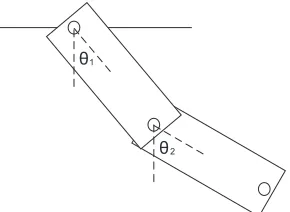
We applied DirectLiNGAM and ICA-LiNGAM on a data set created from a physical system called a double-pendulum, a pendulum with another pendulum attached to its end (Meirovitch, 1986) as in Figure 3. The data set was first used in Kawahara et al. (2011). The raw data consisted of four time series provided by Ibaraki University (Japan) filming the pendulum system with a high-speed video camera at every 0.01 second for 20.3 seconds and then reading out the position using an image analysis software. The four variables wereθ1: the angle between the top limb and the vertical,θ2: the angle between the bottom limb and the vertical,ω1: the angular speed ofθ1 or ˙θ1andω2: the angular speed ofθ2 or ˙θ2. The number of time points was 2035. The data set is available on the web:http://www.ar.sanken.osaka-u.ac.jp/˜inazumi/data/furiko.html.
1
2
Figure 3: Abstract model of the double-pendulum used in Kawahara et al. (2011).
Æ1
Æ2
Ö1
Ö
2Æ1
Æ2
Ö1
Ö
2DirectLiNGAM ICA-LiNGAM
Figure 4: Left: The estimated network by DirectLiNGAM. Only significant directed edges are shown with 5% significance level. Right: The estimated network by ICA-LiNGAM. No significant directed edges were found with 5% significance level.
Æ1
Æ2
Ö1
Ö
2PC GES
Æ1
Æ2
Ö1
Ö
2Figure 5: Left: The estimated network by PC algorithm with 5% significance level. Right: The estimated network by GES. An undirected edge between two variables means that there is a directed edge from a variable to the other or the reverse.
very small. Further, in practice, it was reasonable to assume that there were no latent confounders (Kawahara et al., 2011).
preprocessed data. The estimated adjacency matrices B ofθ1,θ2,ω1andω2were as follows:
DirectLiNGAM :
θ1 θ2 ω1 ω2
θ1 0 0 0 0
θ2 −0.23 0 0 0 ω1 90.39 −2.88 0 0 ω2 5.65 94.64 −0.11 0
,
ICA−LiNGAM :
θ1 θ2 ω1 ω2
θ1 0 0 0 0
θ2 1.45 0 0 0
ω1 108.82 −52.73 0 0 ω2 216.26 112.50 −1.89 0
.
The estimated orderings by DirectLiNGAM and ICA-LiNGAM were identical, but the estimated connection strengths were very different. We further computed their 95% confidence intervals by using bootstrapping (Efron and Tibshirani, 1993) with the number of bootstrap replicates 10000. The estimated networks by DirectLiNGAM and ICA-LiNGAM are graphically shown in Figure 4, where only significant directed edges (direct causal effects) bi j are shown with 5% significance
level.3 DirectLiNGAM found that the angle speedsω1andω2were determined by the angles θ1 orθ2, which was consistent with the domain knowledge. Though the directed edge fromθ1toθ2 might be a bit difficult to interpret, the effect ofθ1 onθ2was estimated to be negligible since the coefficient of determination (Bollen, 1989) of θ2, that is, 1−var( ˆe2)/var( ˆθ2), was very small and was 0.01. (The coefficient of determination ofω1and that ofω2were 0.46 and 0.49, respectively.) On the other hand, ICA-LiNGAM could not find any significant directed edges since it gave very different estimates for different bootstrap samples.
For further comparison, we also tested two conventional methods (Spirtes and Glymour, 1991; Chickering, 2002) based on conditional independences. Figure 5 shows the estimated networks by PC algorithm (Spirtes and Glymour, 1991) with 5% significance level and GES (Chickering, 2002) with the Gaussianity assumption. We used the Tetrad IV4 to run the two methods. PC algorithm found the same directed edge fromθ1onω1as DirectLiNGAM did, but did not found the directed edge fromθ2onω2. GES found the same directed edge fromθ1onθ2as DirectLiNGAM did, but did not find that the angle speedsω1andω2were determined by the anglesθ1orθ2.
We also computed the 95% confidence intervals of the total causal effects ai j using bootstrap.
DirectLiNGAM found significant total causal effects fromθ1onθ2, fromθ1onω1, fromθ1onω2, fromθ2 onω1, and fromθ2 onω2. These significant total effects would also be reasonable based on similar arguments. ICA-LiNGAM only found a significant total causal effect fromθ2onω2.
Overall, although the four variables θ1, θ2,ω1 andω2 are likely to be nonlinearly related ac-cording to the domain knowledge (Meirovitch, 1986; Kawahara et al., 2011), DirectLiNGAM gave interesting results in this example.
5.2 Application to Sociology Data
We analyzed a data set taken from a sociological data repository on the Internet called General Social Survey (http://www.norc.org/GSS+Website/). The data consisted of six observed
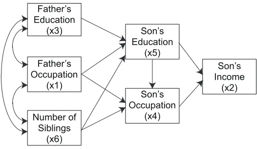
Father Õs Education (x3) Father Õs Occupation (x1) SonÕs Education (x5) Number of Siblings (x6) SonÕs Occupation (x4) SonÕs Income (x2)
Figure 6: Status attainment model based on domain knowledge (Duncan et al., 1972). A directed edge between two variables in the figure means that there could be a directed edge be-tween the two. A bi-directed edge bebe-tween two variables means that the relation is not modeled. For instance, there could be latent confounders between the two, there could be a directed edge between the two, or the two could be independent.
ables, x1: father’s occupation level, x2: son’s income, x3: father’s education, x4: son’s occupation level, x5: son’s education, x6: number of siblings. (x6is discrete but is relatively close to be contin-uous since it is an ordinal scale with many points.) The sample selection was conducted based on the following criteria: i) non-farm background; ii) ages 35 to 44; iii) white; iv) male; v) in the labor force at the time of the survey; vi) not missing data for any of the covariates; vii) years 1972-2006. The sample size was 1380. Figure 6 shows domain knowledge about their causal relations (Duncan et al., 1972). As shown in the figure, there could be some latent confounders between x1and x3, x1 and x6, or x3and x6. An objective of this example was to see how our method behaves when such a model assumption of LiNGAM could be violated that there is no latent confounder.
The estimated adjacency matrices B by DirectLiNGAM and ICA-LiNGAM were as follows:
DirectLiNGAM :
x1 x2 x3 x4 x5 x6
x1 0 0 3.19 0.10 0.41 0.21
x2 33.48 0 452.84 422.87 1645.45 347.96
x3 0 0 0 0 0.55 −0.18
x4 0 0 0.17 0 4.61 −0.19
x5 0 0 0 0 0 −0.12
x6 0 0 0 0 0 0
,
ICA−LiNGAM :
x1 x2 x3 x4 x5 x6
x1 0 0 0.93 0 −0.68 −0.20
x2 50.70 0 −31.82 200.84 65.63 336.04
x3 0 0 0 0 0.24 −0.27
x4 0.17 0 −0.40 0 −0.14 −0.14
x5 0 0 0 0 0 0
x6 0 0 0 0 −0.08 0
We subsequently pruned redundant directed edges bi j in the full DAGs by repeatedly
apply-ing a sparse method called Adaptive Lasso (Zou, 2006) on each variable and its potential parents. See Appendix A for some more details of Adaptive Lasso. We used a matlab implementation in Sj¨ostrand (2005) to run the Lasso. Then we obtained the following pruned adjacency matrices B:
DirectLiNGAM :
x1 x2 x3 x4 x5 x6
x1 0 0 3.19 0 0 0
x2 0 0 0 422.87 0 0
x3 0 0 0 0 0.55 0
x4 0 0 0 0 4.61 0
x5 0 0 0 0 0 −0.12
x6 0 0 0 0 0 0
,
ICA−LiNGAM :
x1 x2 x3 x4 x5 x6
x1 0 0 0.93 0 0 0
x2 0 0 0 200.84 0 0
x3 0 0 0 0 0.24 0
x4 0 0 0 0 −0.14 0
x5 0 0 0 0 0 0
x6 0 0 0 0 −0.08 0
.
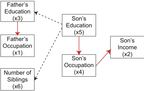
The estimated networks by DirectLiNGAM and ICA-LiNGAM are graphically shown in Fig-ure 7 and FigFig-ure 8, respectively. All the directed edges estimated by DirectLiNGAM were reason-able to the domain knowledge other than the directed edge from x5: son’s education to x3: father’s education. Since the sample size was large and yet the estimated model was not fully correct, the mistake on the directed edge between x5and x3might imply that some model assumptions might be more or less violated in the data. ICA-LiNGAM gave a similar estimated network but did one more mistake that x6: number of siblings is determined by x5: son’s education.
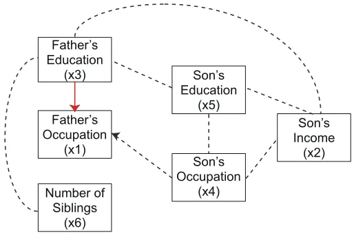
Further, Figure 9 and Figure 10 show the estimated networks by PC algorithm with 5% signif-icance level and GES with the Gaussianity assumption. Both of the conventional methods did not find the directions of many edges. The two conventional methods found a reasonable direction of the edge between x1: father’s occupation and x3: father’s education, but they gave a wrong direction of the edge between x1: father’s occupation and x4: son’s occupation.
6. Conclusion
Father Õs Education
(x3)
Father Õs Occupation
(x1)
SonÕs Education
(x5)
Number of Siblings
(x6)
SonÕs Occupation
(x4)
SonÕs Income
(x2)
Figure 7: The estimated network by DirectLiNGAM and Adaptive Lasso. A red solid directed edge is reasonable to the domain knowledge.
Father Õs Education
(x3)
Father Õs Occupation
(x1)
SonÕs Education
(x5)
Number of Siblings
(x6)
SonÕs Occupation
(x4)
SonÕs Income
(x2)
Figure 8: The estimated network by ICA-LiNGAM and Adaptive Lasso. A red solid directed edge is reasonable to the domain knowledge.
(Hoyer et al., 2008; Kawahara et al., 2010) or nonlinear relations (Hoyer et al., 2009; Mooij et al., 2009) and iv) comparison of our method and related algorithms on many other real-world data sets.
Acknowledgments
Father Õs Education
(x3)
Father Õs Occupation
(x1)
SonÕs Education
(x5)
Number of Siblings
(x6)
SonÕs Occupation
(x4)
SonÕs Income
(x2)
Figure 9: The estimated network by PC algorithm with 5% significance level. An undirected edge between two variables means that there is a directed edge from a variable to the other or the reverse. A red solid directed edge is reasonable to the domain knowledge.
Father Õs Education
(x3)
Father Õs Occupation
(x1)
SonÕs Education
(x5)
Number of Siblings
(x6)
SonÕs Occupation
(x4)
SonÕs Income
(x2)
Figure 10: The estimated network by GES. An undirected edge between two variables means that there is a directed edge from a variable to the other or the reverse. A red solid directed edge is reasonable to the domain knowledge.
as a Foundation for the Sciences’. A.H. was partially supported by the Academy of Finland Centre of Excellence for Algorithmic Data Analysis.
Appendix A. Adaptive Lasso
We very briefly review the adaptive Lasso (Zou, 2006), which is a variant of the Lasso (Tibshirani, 1996). See Zou (2006) for more details. The adaptive Lasso is a regularization technique for variable selection and assumes the same data generating process as LiNGAM:
xi=
∑
k(j)<k(i)
A big difference is that the adaptive Lasso assumes that the set of such potential parent variables xj that k(j)<k(i)is known and LiNGAM estimates the set of such variables. The adaptive Lasso
penalizes connection strengths bi j in L1penalty by minimizing the objective function defined as:
xi−k(j
∑
)<k(i)bi jxj 2+λ
∑
k(j)<k(i)
|bi j|
|ˆbi j|γ
,
whereλandγare tuning parameters and ˆbi j is a consistent estimate of bi j. In Zou (2006), it was
suggested to select the tuning parameters by five-fold cross validation and to obtain ˆbi j by ordinary
least squares regression. The adaptive Lasso has a very attractive property that it asymptotically selects the right set of such variables xjthat bi j is not zero, where k(j)<k(i).
References
S. Amari. Natural gradient learning works efficiently in learning. Neural Computation, 10:251–276, 1998.
F. R. Bach and M. I. Jordan. Kernel independent component analysis. Journal of Machine Learning Research, 3:1–48, 2002.
K. A. Bollen. Structural Equations with Latent Variables. John Wiley & Sons, 1989.
D. Chickering. Optimal structure identification with greedy search. Journal of Machine Learning Research, 3:507–554, 2002.
P. Comon. Independent component analysis, a new concept? Signal Processing, 36:62–83, 1994.
G. Darmois. Analyse g´en´erale des liaisons stochastiques. Review of the International Statistical Institute, 21:2–8, 1953.
O. D. Duncan, D. L. Featherman, and B. Duncan. Socioeconomic Background and Achievement. Seminar Press, New York, 1972.
B. Efron and R. Tibshirani. An Introduction to the Bootstrap. Chapman & Hall, New York, 1993.
J. Eriksson and V. Koivunen. Identifiability, separability, and uniqueness of linear ICA models. IEEE Signal Processing Letters, 11:601–604, 2004.
A. Gretton and L. Gy¨orfi. Consistent nonparametric tests of independence. Journal of Machine Learning Research, 11:1391–1423, 2010.
A. Gretton, O. Bousquet, A. J. Smola, and B. Sch¨olkopf. Measuring statistical dependence with Hilbert-Schmidt norms. In Algorithmic Learning Theory: 16th International Conference (ALT2005), pages 63–77. 2005.
P. O. Hoyer, S. Shimizu, A. Kerminen, and M. Palviainen. Estimation of causal effects using linear non-gaussian causal models with hidden variables. International Journal of Approximate Reasoning, 49(2):362–378, 2008.
P. O. Hoyer, D. Janzing, J. Mooij, J. Peters, and B. Sch¨olkopf. Nonlinear causal discovery with additive noise models. In D. Koller, D. Schuurmans, Y. Bengio, and L. Bottou, editors, Advances in Neural Information Processing Systems 21, pages 689–696. 2009.
A. Hyv¨arinen. New approximations of differential entropy for independent component analysis and projection pursuit. In Advances in Neural Information Processing Systems, volume 10, pages 273–279. 1998.
A. Hyv¨arinen. Fast and robust fixed-point algorithms for independent component analysis. IEEE Transactions on Neural Networks, 10:626–634, 1999.
A. Hyv¨arinen, J. Karhunen, and E. Oja. Independent Component Analysis. Wiley, New York, 2001.
A. Hyv¨arinen, K. Zhang, S. Shimizu, and P. O. Hoyer. Estimation of a structural vector autoregres-sive model using non-Gaussianity. Journal of Machine Learning Research, 11:1709–1731, May 2010.
T. Inazumi, S. Shimizu, and T. Washio. Use of prior knowledge in a non-Gaussian method for learn-ing linear structural equation models. In Proc. 9th International Conference on Latent Variable Analysis and Signal Separation (LVA/ICA2010), pages 221–228, 2010.
M. Kalisch and P. B¨uhlmann. Estimating high-dimensional directed acyclic graphs with the PC-algorithm. Journal of Machine Learning Research, 8:613–636, 2007.
Y. Kawahara, K. Bollen, S. Shimizu, and T. Washio. GroupLiNGAM: Linear non-Gaussian acyclic models for sets of variables. arXiv:1006.5041, June 2010.
Y. Kawahara, S. Shimizu, and T. Washio. Analyzing relationships among ARMA processes based on non-Gaussianity of external influences. Neurocomputing, 2011. Forthcoming.
A. Kraskov, H. St¨ogbauer, and P. Grassberger. Estimating mutual information. Physical Review E, 69(6):066138, 2004.
G. Lacerda, P. Spirtes, J. Ramsey, and P. O. Hoyer. Discovering cyclic causal models by indepen-dent components analysis. In Proceedings of the 24th Conference on Uncertainty in Artificial Intelligence (UAI2008), pages 366–374, 2008.
A. Londei, A. D’Ausilio, D. Basso, and M. O. Belardinelli. A new method for detecting causality in fMRI data of cognitive processing. Cognitive processing, 7(1):42–52, March 2006.
L. Meirovitch. Elements of Vibration Analysis (2nd ed.). McGraw-Hill, 1986.
J. Pearl. Causality: Models, Reasoning, and Inference. Cambridge University Press, 2000. (2nd ed. 2009).
R. O. Rhein and K. Strimmer. From correlation to causation networks: a simple approximate learning algorithm and its application to high-dimensional plant gene expression data. BMC Systems Biology, 1:1–37, 2007.
S. Shimizu, P. O. Hoyer, A. Hyv¨arinen, and A. Kerminen. A linear non-gaussian acyclic model for causal discovery. Journal of Machine Learning Research, 7:2003–2030, 2006.
S. Shimizu, A. Hyv¨arinen, Y. Kawahara, and T. Washio. A direct method for estimating a causal ordering in a linear non-gaussian acyclic model. In Proceedings of the 25th Conference on Un-certainty in Artificial Intelligence (UAI2009), Montreal, Canada, pages 506–513. AUAI Press, 2009.
R. Silva, R. Scheines, C. Glymour, and P. Spirtes. Learning the structure of linear latent variable models. Journal of Machine Learning Research, 7:191–246, Feb 2006.
K. Sj¨ostrand. Matlab implementation of LASSO, LARS, the elastic net and SPCA, June 2005. URL http://www2.imm.dtu.dk/pubdb/p.php?3897. Version 2.0.
W. P. Skitovitch. On a property of the normal distribution. Doklady Akademii Nauk SSSR, 89: 217–219, 1953.
Y. Sogawa, S. Shimizu, Y. Kawahara, and T. Washio. An experimental comparison of linear non-Gaussian causal discovery methods and their variants. In Proceedings of 2010 International Joint Conference on Neural Networks (IJCNN2010), pages 768–775, 2010.
P. Spirtes and C. Glymour. An algorithm for fast recovery of sparse causal graphs. Social Science Computer Review, 9:67–72, 1991.
P. Spirtes, C. Glymour, and R. Scheines. Causation, Prediction, and Search. Springer Verlag, 1993. (2nd ed. MIT Press 2000).
R. Tibshirani. Regression shrinkage and selection via the lasso. Journal of Royal Statistical Society: Series B, 58(1):267–288, 1996.