DOI: 10.5098/hmt.7.40 ISSN: 2151-8629
1
Frontiers in Heat and Mass Transfer
Available at www.ThermalFluidsCentral.org
MODELLING OF PHASE CHANGE WITH NON-CONSTANT
DENSITY USING XFEM AND A LAGRANGE MULTIPLIER
Dave Martina,b,†, Hicham Chaoukia,b, Jean-Loup Roberta, Donald Zieglerc, Mario Fafarda,b
a
Department of Civil and Water Engineering, Laval University, Quebec, QC, G1V 0A6, Canada b
NSERC/Alcoa Industrial Research Chair MACE3and Aluminium Research Centre - REGAL, Laval University, Quebec, QC, G1V 0A6, Canada c
Alcoa Primary Metals, Alcoa Technical Center, 100 Technical Drive, Alcoa Center, PA, 15069-0001, USA
ABSTRACT
Atwophasemodelfortwo-dimensionalsolidificationproblemswithvariabledensitieswasdevelopedbycouplingtheStefanproblemwiththeStokes problemandapplyingamassconservingvelocityconditiononthephasechangeinterface.Theextendedfiniteelementmethod(XFEM)wasusedto capturethestrongdiscontinuityofthevelocityandpressureaswellasthejumpinheatfluxatthei nterface.Themeltingtemperatureandvelocity conditionwereimposedontheinterfaceusingaLagrangemultiplierandthepenalizationmethod,respectively.Theresultingformulationswerethen coupledusingafixedpointiterationa lgorithm.Threeexampleswereinvestigatedandtheresultswerecomparedtonumericalresultscomingfrom acommercialsoftwareusingALEtechniquestotrackthesolid/liquidinterface. Themodelwasabletoreproducethebenchmarksimulationswhile maintainingasharpphasechangeinterfaceandconservingmass.
Keywords:Phasechange,XFEM,Lagrangemultiplier,Non-constantdensity
1. INTRODUCTION
The finite element methodReddy(2006) has been extensively studied and successfully used in a wide variety of scenarios involving continu-ous media but particular situations still offer a challenge, such as material and geometrical discontinuities. This makes the finite element method ill suited to solve problems involving discontinuities that are part of the solution or moving with time. The Stefan problemNedjar(2002); Beck-ermannet al.(1999);Helenbrook(2013);Özi¸sik(1993) for the isother-mal solidification or melting of a material is one such situation because of the discontinuous heat flux at the phase change interface. The problem is further complicated by the fact that most materials undergo a change in density at the interface, effectively adding a mass flux boundary con-dition. Luckily, the density variation in most materials is small and can be neglectedMorgan(1981);Posteket al.(2008). For certain materials however, the density variation may be quite important, up to 25%. Fur-thermore, many practical applications involve following the total volume of the material or mass flow. In these situations, neglecting the density change significantly hinders the use of numerical models.
To handle such problems involving discontinuities, the extended fi-nite element methodBelytschkoet al.(2001);Dolbowet al.(2000); Be-lytschko et al. (2009) was developed, based on the partition of unity methodBabuska and Melenk(1997);Dolbowet al.(2000);Melenk and Babuska(1996). Using carefully selected functionsψ(x, t), the technique adds degrees of freedom that will “enrich" the interpolation and allows the solution to adopt a non-linear (discontinuous) behavior. The partic-ular type of behavior is determined by the enrichment functionψ(x, t), knowna priori. Only nodes having support cut by the interface have a modified behavior must be enriched. Consequently, the additional
com-†
Corresponding author. Email: [email protected]
putational costs are local to the interface. The interface geometry is stored and transported in a computationally efficient manner, most commonly using the level set methodOsher and Sethian(1988);Osher and Fedkiw (2001).
Numerous extended finite element models for the solutions of the classical (diffusive) Stefan problem are found in the literature Chessa et al.(2002);Bernauer and Herzog(2011);Merle and Dolbow(2002); Jiet al.(2002). More complex models involving convection with con-stant density have also been developed using different numerical tech-niquesZabaraset al.(2006);Vynnycky and Kimura(2007);Brentet al. (1988). Particularly, a fully XFEM Stefan/Navier-Stokes model was used byMartin(2016). Models including the density variation are more un-commonYoo and Tack(1991). A straight-forward strategy to include the non-constant material densities is to use a moving-mesh algorithm such as the one found in the commercial code Comsol. This algorithm defines the phase change interface on a set of nodes, allowing the mass conserva-tion boundary condiconserva-tion to be easily applied. However, the moving mesh adds considerable computational costs caused by the increase in degrees of freedom of the overall problem and the remeshing procedure required when the mesh becomes too distorted. These costs may hinder the use of a moving mesh algorithms in large scale multi-physical simulations which often have a large amount of degrees of freedom.
DOI: 10.5098/hmt.7.40 ISSN: 2151-8629 the phase change interface is handled by applying a velocity boundary
condition.
The paper is divided as follows. The governing equations for the Stefan and Stokes problems are described in section2. The finite ele-ment formulation, level set problem and details concerning the interface movement and extended finite element method are described in section
3. Benchmark examples are then solved in section4to validate the al-gorithm. To this end, the commercial finite element simulation software Comsol was used with a moving mesh algorithm to capture the interface movement. Finally, the paper ends with some concluding remarks.
2. GOVERNING EQUATIONS 2.1. Stefan Problem Formulation
Consider a domainΩwith an initial temperatureT(x, t0)and interfaceΓ
separating solid (Ωs) and liquid (Ωl) phases with different thermal
prop-erties and densities. We suppose that the material has an isothermal phase change at some melting temperatureTm. Applying the conservation of
energy inΩresults in the following equationsÖzi¸sik(1993):
(ρcp)s
∂T
∂t − ∇ ·(ks∇T) = 0 x∈Ωs (1a)
(ρcp)l
∂T
∂t +v· ∇T
− ∇ ·(kl∇T) = 0 x∈Ωl (1b)
T−Tm= 0 x∈Γ (1c)
T = ˆT x∈ΓD (1d)
−k∇T·n= ˆq x∈ΓN (1e)
wherecpis the specific heat,kthe thermal conductivity,ρthe density,
vthe liquid phase velocity. Subscriptslandsindicate liquid and solid phases, respectively. Additionally, the melting temperature is applied on the solid-liquid interface (1c). Dirichlet and Neumann boundary condi-tions away from the interface are applied on∂Ω = ΓN ∪ ΓDas usual
(1d,1e).
Conservation of energy at the interface requires that the jump in heat flux normal to the interface (caused by the imposition of the melting tem-perature) be related to the rate of solidification or melting of the material as described inÖzi¸sik(1993):
[[−k∇T]]·nΓ= (kl∇Tl−ks∇Ts)·nΓ=ρsLvΓ x∈Γ (2)
whereLis the latent heat andvΓthe normal interface velocityÖzi¸sik
(1993). The normal vector nΓ points from the liquid to solid phase,
meaning that the interface velocity is positive for melting and negative for solidification.
Tracking the moving interface is done using the level set method Osher and Fedkiw(2001);Osher and Sethian(1988);Osher and Fedkiw (2003). The principle behind this method is to introduce a signed distance function to the interface,φ(x, t), defined as followsOsher and Fedkiw (2003):
φ(x, t) = min xΓ∈Γ
|x−xΓ(t)|sign(nΓ·(x−xΓ(t))) x∈Ω (3)
The interface is then easily identified as the set of points whereφ(x, t) = 0. In this work, the level set field is constructed so that the liquid phase is on the positive side of the interface (i.e.x∈Ωlifφ(x, t)>0).
2.2. Stokes Problem formulation
In the present study, the liquid phase velocityvis governed by the Stokes problem for viscous incompressible fluids:
ρl
∂v
∂t =∇ ·σ x∈Ωl (4a)
∇ ·v= 0 x∈Ωl (4b)
v=ρl−ρs
ρl
vΓnΓ x∈Γ (4c)
v= ˆv x∈ΓD (4d)
σ·n= ˆσ x∈ΓN (4e)
σ=−pI+ 2µD(v) (4f)
D(v) =1 2
∇v+∇vT
(4g)
wherepis the pressure,µthe viscosity andD(v)the rate of deformation tensor. The convection term in the complete Navier-Stokes equations was neglected, leading to two linear systems of equations for the heat transfer and fluid flow problems. The only non-linearity is in the coupling terms between the two problems: the convective heat transfer and interface ve-locity.
The variation in density between the solid and liquid phases creates a mass flux at the interface, which is a function of the interface velocity and specific phase densities (equation (4c)). The other physical proper-ties are assumed constant. The initial velocity fieldv(x, t0)is assumed
divergence-free with a given initial pressure fieldp(x, t0). Dirichlet and
Neumann boundary conditions away from the interface are applied on
∂Ω = ΓN ∪ ΓDas usual (4d,4e).
2.3. Enriched Interpolation Scheme
The phase change problem is characterized by the jump in the heat flux which is caused by the temperature gradient discontinuity. However, the application of the interface boundary condition (1c) implies that the tem-perature is continuous at the interface. Such a weak discontinuity can be handled using the extended finite element method. To this end, the following interpolation scheme is usedChessaet al.(2002):
T(x, t) =X
i∈I
NiT(x)Ti(t) +
X
j∈J
NjT(x)ψ T j(x, t)T
∗
j(t) (5a)
ψTj(x, t) =|φ(x, t)| − |φ(xj, t)| (5b)
whereNT are the standard interpolation functions,TiandTj∗the
stan-dard and enriched degrees of freedom, respectively, andψTj(x, t)the
en-richment function, based on the absolute value of the level set field. A more compact way to write expression (5) is by using the standard matrix form
T(x, t) =hNTi{T} (6a)
hNTi=hN1T, ..., N
T nI, N
T
1ψ
T
1, ..., N
T nJψ
T
nJi (6b)
{T}=hT1, ..., TnI, T1∗, ..., T ∗
nJi
T
(6c)
wherenI and nJ are the number of standard and enriched nodes,
re-spectively. When using (5) special attention must be given to elements containing enriched nodes that are not cut by the interface, called blend-ing elements. A modified interpolation scheme must be used in these elements to maintain an optimal convergence rate, as described inFries (2008);Shibanuma and Utsunomiya(2009).
DOI: 10.5098/hmt.7.40 ISSN: 2151-8629 for the Lagrange multiplier is given by:
λ(x, t) =X
i∈I
Niλ(x)λi(t) +
X
j∈J
Njλ(x)ψ λ j(x, t)λ
∗
j(t) (7a)
ψλj(x, t) =H(φ(x, t))−H(φ(xj, t)) (7b)
H(x, t) = (
1 ifφ(x, t)<0
0 ifφ(x, t)>0 (7c)
where H is the Heaviside function.
Following (6), the Lagrange multiplier may be rewritten in two di-mensions as
λ(x, t) = [Nλ]hλiT
[Nλ] =
Nλ
1... NnλIN
λ
1ψ1λ... NnλJψ
λ
nJ 0 ... 0 0 ... 0
0 ... 0 0 ... 0 N1λ... NnλIN1λψ1λ... NnλJψnλJ
hλi=hλx1, ... , λ
x nI, λ
x∗ 1 , ..., λ
x∗
nJ, λ
y
1, ... , λ
y nI, λ
y∗ 1 , ..., λ
y∗
nJi
where[Nλ]is the matrix of interpolation functions.
The Navier-Stokes equations are valid (and solved) in the liquid phase only. For this purpose, the fluid-structure interaction approach, proposed inGerstenberger and Wall(2008), is used. Therefore, the ve-locity and pressure fields can be interpolated using the following scheme:
v(x, t) =X
i∈I
Niv(x)ψ v
(x, t)vi(t) (9a)
p(x, t) =X
i∈I
Nip(x)ψv(x, t)pi(t) (9b)
ψv(x, t) = (
1 ifφ(x, t)>0
0 ifφ(x, t)<0 (9c) Following (6) and (2.3), the velocity and pressure fields may be rewritten as:
v(x, t) = [Nv]{v} (10a)
p(x, t) =hNpi{p} (10b)
[Nv] =
N1vψv1 ... NnvIψ
v
nI 0 ... 0
0 ... 0 N1vψ1v ... NnvIψnvI
(10c)
{v}=hvx1, ... , v
x nI, v
y
1, ... , v
y nIi
T
(10d)
hNpi=hN1pψ
v
1, ..., N
p nIψ
v
nIi (10e)
{p}=hp1, ..., pnIi
T
(10f)
According to this interpolation scheme, the solid part of the domain if ignored. Also, enriched degrees of freedom are not required because no new information (behavior) is introduced. All velocity and pressure de-grees of freedom whose support is completely inside the solid domain are removed from the system of equations.
3. NUMERICAL IMPLEMENTATION 3.1. Stefan Problem
The weak form of the energy conservation equations (1a,1b) is
Z
Ω δT ρcp
∂T ∂t dΩ +
Z
Ωl
δT ρlcpv· ∇TdΩ +
Z
Ω
∇δT k∇TdΩ
(11a)
− Z
Γ
δTλ·nΓdΓ = 0
Z
Ω δλ·
1
kλ+∇T
dΩ−
Z
Γ
δλ·nΓ(T−Tm) dΓ = 0 (11b)
whereδT andδλare the test functions. The method used in this work to impose the melting temperature on the interface is the stable Lagrange
multiplier used inMartinet al.(2016) and originally developed in Ger-stenberger and Wall(2010);Baigeset al.(2012). The Lagrange multi-plier is defined as a vectorial flux and interpolated on the same mesh as the temperature field. The projection of this secondary variable on the in-terface is then used as a scalar Lagrange multiplier to impose the melting temperature. The Neumann boundary condition has been omitted for the sake of clarity.
Using a backward Euler scheme for the time derivative of T in (11) givesFries and Zilian(2009):
Z
Ω
δTn+1(ρcpT)
n+1−(ρc
pT)n
∆t dΩ+
Z
Ωl
δTn+1(ρcp)n+1vn+1· ∇Tn+1dΩ+
Z
Ω
∇δTn+1kn+1∇Tn+1dΩ− Z
Γ
δTn+1λn+1·nΓdΓ = 0
(12a)
Z
Ω δλn+1·
1
kλ
n+1
+∇Tn+1
dΩ−
Z
Γ
δλn+1·nΓ Tn+1−Tm
dΓ = 0
(12b)
wherenindicates the previous time step.
After replacing T andλwith their approximations we obtain the system of equations
1
∆t[M] + [C] + [K] −[L]
[Q]−[L]T [M λ]
{T}n+1 {λ}n+1
(13a)
=
1
∆t[M]
∗ 0
0 0
{T}n
{λ}n
−
0 {fλ}
[M] =X
e
Z
Ωe
{NT}n+1(ρcp)n+1hNTin+1dΩ (13b)
[M]∗=X
e
Z
Ωe
{NT}n+1(ρcp)nhNTindΩ (13c)
[C] =X
e
Z
Ωe
l
{NT}n+1(ρcp)n+1vn+1[BT]n+1dΩ (13d)
[K] =X
e
Z
Ωe
([BT]T)n+1kn+1[BT]n+1dΩ (13e)
[Mλ] =
X
e
Z
Ωe
1
kn+1([Nλ]
T
)n+1[Nλ]n+1dΩ (13f)
[Q] =X
e
Z
Ωe
([Nλ]T)n+1[B]n+1dΩ (13g)
[L] =X
e
Z
Γe
{NT}n+1[Nλ]n+1nΓdΓ (13h)
{fλ}= X
e
Z
Γe
([Nλ]T)n+1·nΓTmdΓ (13i)
whereBnij+1 = ∂Njn+1
∂xi is the gradient matrix and the {} brackets are
used to indicate a vector transpose. In elements which are not cut by the interface, the boundary condition is removed and the system reduces to:
1
∆t[M] + [C] + [K] 0
[Q] [Mλ]
{T}n+1 {λ}n+1
=
1
∆t[M]
∗ 0
0 0
{T}n
{λ}n
DOI: 10.5098/hmt.7.40 ISSN: 2151-8629
3.2. Stokes Problem
The weak form of the Stokes problem (4) is given as follows
Z
Ωl
δv·ρl
∂v
∂t dΩ +
Z
Ωl
2µ D(δv) :D(v) dΩ− Z
Ωl
(∇ ·δv)pdΩ = 0 Z
Ωl
δp∇ ·vdΩ = 0 (15a)
whereδvandδpare the test functions for the velocity and pressure, re-spectively. The Neumann boundary condition has been omitted for the sake of clarity. Using a backward Euler scheme for the time derivative of
vin (15) gives the system of equationsFries and Zilian(2009):
Z
Ωl
δvn+1·
(ρlv)n+1−(ρlv)n
∆t
dΩ +
Z
Ωl
2µD(δvn+1) :D(vn+1) dΩ
− Z
Ωl
∇ ·δvn+1pn+1dΩ = 0 (16a)
Z
Ωl
δpn+1∇ ·vn+1dΩ = 0 (16b)
Substituting the approximation for the velocity and pressure fields into (16) leads to the system of equations:
[K] −[D] [D]T 0
{v}n+1 {p}n+1
=
[M]∗ 0
0 0
{v}n
{p}n
(17a)
[K] = [M] +
[A11] [A12] [A12]T [A22]
(17b)
[M] = 1 ∆t
X
e
Z
Ωe
([Nv]T)n+1ρl[Nv]n+1dΩ (17c)
[M]∗= 1 ∆t
X
e
Z
Ωe
([Nv]T)n+1ρl[Nv]ndΩ (17d)
[A11] = X e Z Ωe 2µ
{Bx}n+1hBxin+1+
1 2{By}
n+1 hByin+1
dΩ
(17e)
[A22] = X e Z Ωe 2µ 1 2{Bx}
n+1
hBxin+1+{By}n+1hByin+1
dΩ
(17f)
[A12] = X e Z Ωe 2µ 1 2{By}
n+1h Bxin+1
dΩ (17g)
[D] =X
e
Z
Ωe
hhBxin+1hByin+1iThNpin+1dΩ (17h)
hBxii
n+1 =∂hN
v
1ψ1v, ..., NnvIψ
v nIi
n+1 ∂xi
(17i)
The mass flux interface boundary condition is imposed using the penalty methodChessaet al.(2002);Bernauer and Herzog(2011). This tech-nique multiplies the residual form of equation (4c) by a very large penal-ization parameterβand introduces it in the finite element formulation of the momentum equation. This method is simple to implement and has proven to be robust for a variety of problems. The formulation for ele-ments intersected by the interface becomes:
[K0] −[D] [D]T 0
{v}n+1 {p}n+1
=
[M]∗ 0
0 0
{v}n
{p}n
+
{fnp+1}
0
(18a)
[K0] = [K] + [P] (18b)
[P] =X
e
Z
Γe
([Nv]T)n+1β[Nv]n+1dΓ (18c)
{fnp+1}=
X
e
Z
Γe
([Nv]T)n+1β
ρl−ρs
ρl
vΓnΓ
dΓ (18d)
To solve the system of equations (17)-(18) the interpolation func-tions for the velocity and pressure fields must satisfy the LBB condi-tionBabuska(1969);Brezzi(1974). In this work, a pair of stable Q2-Q1 quadrilateral elements was used for the velocity and pressure fields, re-spectively.
The validation problems presented in the results section are com-pared with the solution obtained through the commercial finite element code Comsol where the phase change problem was solved using a mov-ing mesh algorithm (ALE) to capture the interface movement.
The interpolation scheme (9) is known to cause problems when the physical domain (liquid phase) covers a very small area of the node’s supportLanget al.(2014). The small contribution of the concerned de-gree of freedom causes a significant increase in the condition number of the global systemLanget al.(2014), leading to divergent solutions. An efficient solution was developed inLanget al.(2014). When a degree of freedom’s contribution to the system is too small, it is removed from the system. The criteria for removing a degree of freedom isLanget al. (2014)
max
e∈Ei
R
Ωe
l
Ni(x) dΩ
R
ΩeNi(x) dΩ
!−12
> Ttol (19)
whereEiis the set of elements connected to node i,Ωelthe liquid domain
area in the element,Ωethe element area,N
i(x)the interpolation function
andTtol a user defined tolerance value. The greater the value forTtol,
the smaller the contribution of the degree of freedom can be before it is removed.
The stopping criteria (19) is used on a stabilized Q1-Q1inLanget al. (2014), meaning that the velocity and pressure interpolation functions are identical, linear and positive-semidefinite. The quadratic interpolation used for velocity in this work however, is not positive-semidefinite. This means that certain interface positions would lead to near zero integrals in (19) even when the liquid area is large, because the negative-valued areas of the interpolation would cancel out the positive-valued areas. To maintain the original objective of evaluating the relative contribution of the degrees of freedom to the complete element, a modified criteria was used, given by equation
max
e∈Ei
R
Ωe
l
|Ni(x)|dΩ
R
Ωe|Ni(x)|dΩ
!−12
> Ttol (20)
where the absolute value of the interpolation function is used.
InLanget al.(2014) a preconditioner is applied to the global system before solving, allowing the use of a higher value ofTtol while
main-taining an optimal condition number and accurate solution. Considering the relatively heuristic modifications made to the removal of degrees of freedom caused by the use of a Q2-Q1 formulation and to simplify the implementation of our model, the preconditioner was not applied in this work.
The systems of equations (13) and (17) are coupled through the vection and mass flux boundary terms, respectively. To obtain a con-verged solution for both systems, a fixed point iteration scheme is used.
3.3. Level Set Formulation
Once an initial valueφ(x, t0)is defined, the interface movement is
gov-erned by its transport equation
∂φ
∂t +v· ∇φ= ∂φ
∂t +Fk∇φk= 0 (21a)
F= 1
k∇φk∇φ·v (21b)
DOI: 10.5098/hmt.7.40 ISSN: 2151-8629 Equation (21) is solved explicitly (forward Euler scheme) with the
finite element method using a linear interpolation. The weak formulation and time discretization of (21) is given as follows:
Z
Ω δφφ
n+1− φn
∆t dΩ +
Z
Ω
δφFnk∇φnkdΩ = 0 (22)
In most applications, the normal component F is only known onΓ. In order to solve (22) onΩ, a valid value for F must first be constructed on the entire domain using the following problemChessaet al.(2002):
sign(φ)∇F· ∇φ= 0 x∈ Ω (23a)
F(x, t) = ∇φ
k∇φk·vΓ x∈ Γ (23b)
This approach guarantees that theφfield velocity is everywhere nor-mal to the interface and is coherent with the interface’s physically deter-mined velocity. For more details concerning the construction of F see Osher and Fedkiw(2003);Chessaet al.(2002). In this paper, the inter-face velocity is based on the jump in heat flux across the phase change boundary and is described in the following section.
Equation (22) is first order hyperbolic and must be stabilized to min-imize the presence of oscillations in the solutionChessaet al.(2002); Bernauer and Herzog(2011). The GLS method is used hereHugheset al. (1989). The level set method offers several advantages. It is easily ex-tensible to three dimensions and stores the interface location as a scalar variable. Furthermore, the level set field can be defined in a small region surrounding the interface and the level set formulation solved locally, re-ducing the impact on the total simulation computation time. It is also robust enough to handle interface merging and breaking naturallyOsher and Fedkiw(2001).
The main disadvantage of the the level set method is its tendency to deviate from a signed distance function over timeOsher and Fedkiw (2001). This error accumulates with additional time steps and degrades the quality of the solution, particularly the level set gradient near the in-terface. This distortion can be a source of error in the numerical solution of the level set formulation and the physical problem on which it is based. Therefore, it is necessary to reinitializeφ(x, t)regularly to maintain an acceptable solution (k∇φk ≈ 1). Another limitation to the algorithm presented here is the use of an explicit time scheme for the level set for-mulation, which limits the size of the time step. The explicit time step is required in order to determine the nodes to enrich. In other words, the interface position must be determined before systems (13) and (17) are solved.
3.4. Interface velocity calculation
The proper evaluation of the interface velocity is crucial in obtaining a precise and robust modelMartinet al.(2016). For this particular prob-lem, the interface velocity is determined by the jump in heat flux at the interface as described in equation (2). The use of a Lagrange multiplier to impose the melting temperature allows the evaluation of the jump in heat flux directly from the Lagrange fieldλ, given by
vΓ= [[λ]]·ns
ρsL
= (λl−λs)·ns
ρsL
(24)
whereλsandλlare the heat flux at the interface approaching from the
solid and liquid phases, respectively.
The final algorithm can be described as follows. Assuming that a given timetn, solution (Tn,vn,pn,φn) are known, the strategy to solve for (Tn+1,vn+1,pn+1,φn+1) consists in the following steps:
1. Compute the interface velocityvnΓ+1using (24)
2. Construct F on the level set domain by solving (23)
3. Solve forφn+1using (22)
4. Solve the coupled Stefan-Stokes problem:
4.1. Solve forTin+1+1using (13) andv
n+1
i
4.2. Solve forvni+1+1andp
n+1
i+1 using (17) andT
n+1
i+1
5. Evaluate (13) and (17). If both residuals are below the tolerance criteria, go to step6. If not,i=i+ 1and go to step4
6. Settn+1=tnand go to step1.
3.5. Numerical Integration
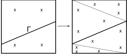
The introduction of discontinuous functions inside elements greatly re-duces the precision of standard Gaussian quadrature and may lead to rank deficient matricesChessaet al.(2002). An accurate but geometrically complex solution is to subdivide elements involving discontinuities into continuous subelementsMoeset al.(1999);Chessaet al.(2002); Ger-stenberger and Wall(2010). Each element is subdivided into a number of subelements (lines, triangles or tetrahedrons), as shown in figure1, to properly fit the contour of the interface (point, line or surface) and ele-ment boundaries. The integral over the entire eleele-mentIeis then the sum
of the integration of each subelementIsusing standard Hammer
quadra-ture. It is important to note that subelements carry no degrees of freedom or interpolation functions. They are only required as a geometrical tool to construct the element integrals.
x x
x x
x
x
x
x x x
x
x x
x x x
Γ
Fig. 1Geometry subdivision for cut element integration In transient problems the location of the quadrature points must change as the interface moves in time, requiring that every cut element be subdivided at each time step. However, the subdivision is applied only to a small number of elements, reducing the overall increase in computa-tional effort required.
In transient problems, the interpolation functions at time steps n
andn+ 1are based on different positions of the interface and are dis-continuous at different places in the element. The integration scheme for the mass matrix (equations (13c) and (17d)) must take both intersec-tions into account when generating the integration subelements to ob-tain optimal convergenceFries and Zilian(2009). This can be difficult and can significantly increases the number of subelements required to fit the geometry. However, previous authors have successfully used inte-gration schemes considering the current interface position onlyChessa et al.(2002);Chessa and Belytschko(2003) and this strategy is used in this work. As suggested inFries and Zilian(2009), the test functions are evaluated using the current time step’s level set values.
4. RESULTS
The Lagrange multiplier formulation used in this work to solve the Ste-fan problem (1) has been previously validated. For details on the specific simulations used and its performance compared to a finite difference ap-proximation of equation (2), the interested reader is referred toMartin et al.(2016).
DOI: 10.5098/hmt.7.40 ISSN: 2151-8629
T = 275
K
p = 0
T = 272
K
T = 273 Ki
q·n=0 v·n=0 q·n=0 v·n=0
x1
(1,0.25)
Γ
Fig. 21D problem definition
Properties Solid Liquid Interface
ρ[kg/m3] 1.0 0.75
-cp[J/kg K] 50 50
-k[W/m K] 0.1 0.1
-ρsL[J/m3] - - 2.5
Tm[K] - - 273.0
µ[kg/s·m] - 10
-Table 1Material properties for 1D and 2D problems
In all cases, the simulations were also run in Comsol, using a moving mesh algorithm (ALE) to account for the displacement of the interface. The Stokes formulation uses aP2−P1formulation, the temperature field
is linear and the Lagrange multiplier is constant per elementMartinet al. (2016). In Comsol, the mesh geometry is quadratic. The results were then compared to the solution obtained using the purely XFEM approach. The Comsol simulations did not include a remeshing step during the simu-lation. An appropriate element size was used to maintain a low enough Peclet number to avoid oscillations in the Stefan problem.
These problems were selected for their relatively simple interface geometry and no reinitialization procedure was applied to the level set field during the simulation. For smooth interface shapes and relatively uniform displacements, the absence of a reinitialization step had little impact on the model’s accuracyMartin(2016). More complex shapes and interface movements would require a reinitialization step as well as a remeshing step in the Comsol algorithm.
4.1. One Dimensional Phase Change Problem
The first benchmark problem is inspired by the one dimensional two phase analytical solution of the Stefan problem in a semi-infinite domain (x >0), taken fromMerle and Dolbow(2002). The thermal properties are constant except for the density and are given in table1. The initial interface is at x = 0.515 m with the liquid phase on the right and solid phase on the left, as shown in figure2. The initial temperature isTm(see
table1). The top and bottom edges are insulated. Att= 0, the temper-ature on the left edge is lowered to 272 K and the right edge is increased to 275 K. For the Navier-Stokes equations, the right boundary is open (no stress) while for the top and bottom edges the following boundary con-dition is applied:v·n= 0. The time step is 0.05 sec,β=1×10⁸and
Ttol=1×10⁸. The mesh contains 180 quadrilateral elements in XFEM
and 196 in Comsol.
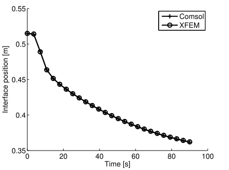
The interface position as a function of time for both Comsol and XFEM algorithms is shown in figure3. The temperature at pointx1over
time is given in figure4for Comsol and XFEM algorithms. The convec-tion velocity (constant in the liquid domain) is shown in figure5for both algorithms. These results show that the XFEM method reproduces the solution obtained through the standard finite element method (Comsol) using the moving mesh algorithm.
4.2. Two Dimensional Phase Change Problem
The second benchmark problem is two dimensional and based on the ana-lytical solution of melting (or freezing) in a corner first solved inRathjen
0 20 40 60 80 100
0.35 0.4 0.45 0.5 0.55
Time [s]
Interface position [m]
Comsol XFEM
Fig. 3Interface position vs time, 1D problem
0 20 40 60 80
273 273.2 273.4 273.6 273.8 274 274.2
Time [s]
Temperature [K]
Comsol XFEM
Fig. 4Temperature at pointx1, 1D problem (see figure2)
0 20 40 60 80
0 0.5 1 1.5 2 2.5 3 3.5x 10
−3
Time [s]
Convection velocity [m/s]
Comsol XFEM
DOI: 10.5098/hmt.7.40 ISSN: 2151-8629
q·n=0 v·n=0
q·n=0 v·n=0 (1,1)
T = 274
K
p = 0
T = 274 K p = 0 T = 273 Ki
x2 x1
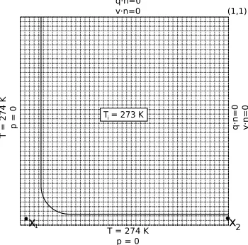
Fig. 62D problem definition.
and Jiji(1971). The thermal properties are constant except for the density and are identical to the first example, given in table1. The initial inter-face is at x = 0.1 m from the left and bottom boundaries, with the liquid phase on the lower left and solid phase on the top right, as shown in fig-ure6. The initial temperature isTm(table1). The top and right edges
are thermally insulated. Att= 0, the temperature on the left and bot-tom boundaries is increased to 274 K. For the Navier-Stokes equations, the left and bottom boundaries are open (no stress). For the top and right boundaries the boundary conditionv·n = 0is applied. The time step is 0.05 sec,β =1×10⁴andT
tol =1×10². The mesh contains 3025
quadrilateral elements in XFEM and 6590 triangle elements in Comsol. The interface position for two different time steps for both Comsol and XFEM algorithms is shown in figure7. The figure shows that the Comsol and XFEM algorthims give identical interface positions.
The temperature profile at the end of the simulation is shown in fig-ure8. Figure9shows the temperature at two pointsx1andx2over time
(see figure6). In both cases, the Comsol and XFEM algorithms are in excellent agreement.
The convection velocity at the final time step for both algorithms is shown in figure10. The velocity is in good agreement in both cases. Figure11shows the fluid velocity at pointsx1andx2over time, showing
good agreement between the two algorithms, although fluctuations are present in the XFEM solution.
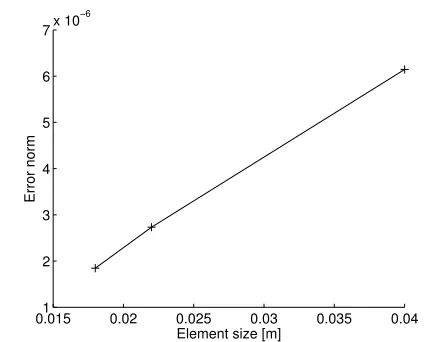
Two distinct causes contribute to these fluctuations. First, the in-terface geometry in XFEM (the level set field) is stored using a linear interpolation. Consequently, the curved interface is approximated by line segments which reduces the accuracy of the solution. Comsol uses a quadratic interpolation for its moving mesh solution, allowing it to re-produce the interface curvature precisely. To validate this hypothesis, a solution was obtained using Comsol and a linear geometry. Using a mesh size similar to figure6, Comsol is unable to produce a converged solu-tion. To obtain a converged solution, over 24 000 triangle elements had to be used and the velocity solution showed small errors, similar to the XFEM solution in figure11. Furthermore, refining the XFEM mesh, thus reducing the error caused by the linear geometry, reduces the error in the solution as can be seen in figure12, where the error norm is defined as
||vC−vX||2,vCis the Comsol velocity andvXthe XFEM velocity over
time at pointx2.
To eliminate this error, a quadratic interface geometry (level set so-lution) can be used for significantly curved interfaces. Note that this does not require the use of a quadratic interpolation of themesh, (as in Com-sol) but the level set field only, limiting the number of additional degrees of freedom required. However, the geometric calculations done using the level set solution (element intersections, normals) becomes more
com-0 0.2 0.4 0.6 0.8 1
0 0.1 0.2 0.3 0.4 0.5 0.6 0.7 0.8 0.9 1
x [m]
y [m]
Comsol t = 5 sec XFEM t = 5 sec Comsol t = 10 sec XFEM t = 10 sec
Fig. 7Interface Comsol and XFEM, 2D problem
plex to implement and the algorithms supposing a linear interpolation must be rewritten. Note that the use of a linear interface may reduce pre-cision but still leads to converged solutions, whereas Comsol struggles to produce converged solutions using a linear mesh interpolation. These findings suggest that the use of the extended finite element method com-bined with the level set method allows for a significant reduction in the number of degrees of freedom required to reach a converged solution, as opposed to Comsol’s moving mesh algorithm.
The second factor is the absence of a preconditioning matrixLang et al.(2014) for the Stokes problem, which meant that lowerTtolvalues
had to be used to obtain a converged solution. This lowTtolvalue causes
important local errors in the velocity near the interface for problematic time steps; the more significant jumps in11are caused by this. To eval-uate the sensitivity of the solution with respect toTtol, the problem was
solved using three different values forTtol:1×100,1×102and1×104.
The velocity norm at pointx1for all threeTtol values compared to the
Comsol solution is given in figure13. As can be seen in the figure, at
Ttol=1×10⁴, certain critical degrees of freedom are not removed and
the error becomes quite significant at 3.5 seconds. This error distorts the level set solution and leads to a divergent solution a few time steps later. AtTtol=1×100too many degrees of freedom are removed and the
sys-tem is unable to reproduce the solution at any time step. Between these two values, atTtol=1×10², the solution shows much smaller errors at
critical time steps and reproduces the correct solution. These results indi-cate that without a preconditionner, the solution can be quite sensitive to a change inTtol.
This source of error can be resolved by adding the preconditioning matrix defined inLanget al.(2014) to the Stokes problem. Although this error impacted only certain time steps, even at the quite lowTtol, more
general applications involving other sources of fluid flow may not be so stableMartin(2016).
4.3. Melting of Cryolite Problem
The last benchmark problem is the melting of cryolite inside a rectangular cavity. The material properties are taken from the FactSage softwareBale et al.(2009) and assumed constant except for the density (see table2). The initial interface is at x = 0.05 m with the liquid phase on the left and solid phase on the right, as shown in figure14. The initial temperature isTm(table2). The top and bottom edges are thermally insulated. The
DOI: 10.5098/hmt.7.40 ISSN: 2151-8629
Fig. 8Temperature at final time step, 2D problem
0 2 4 6 8 10
273 273.2 273.4 273.6 273.8 274
t [s]
T [K]
Comsol pt1 XFEM pt1 Comsol pt2 XFEM pt2
Fig. 9Temperature as function of time atx1andx2, 2D problem (see
figure6)
Fig. 10Velocity at final time step, 2D problem
β=1×10⁴andT
tol =1×101. The mesh contains 1350 quadrilateral
elements in XFEM and 2799 triangle elements in Comsol.
The varying temperature profile along the left and right boundaries will create a variation in heat flux along the interface, causing it to curve. As the solid phase melts, excess mass is released in the liquid phase and leaves the domain through the open boundary in order to fulfill the mass conservation principal.
The interface position for three different time steps for both Com-sol and XFEM algorithms are shown in figure15 and are in excellent agreement. The temperature profile at the end of the simulation is shown in figure16whereas figure17shows the temperature over time at two pointsx1andx2(see figure14). In both cases, the Comsol and XFEM
algorithms are in excellent agreement.
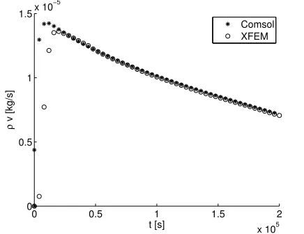
The velocity profile at the end of the simulation is shown in fig-ure18. Figure19shows the fluid velocity at point x1 over time.
Fi-nally, figure20shows the mass flux across the open boundary over time. The graphs clearly indicate that the XFEM algorithm correctly solves the
0 2 4 6 8 10
0 0.005 0.01 0.015 0.02 0.025
t [s]
v [m/s]
Comsol pt1 XFEM pt1 Comsol pt2 XFEM pt2
Fig. 11Velocity as function of time atx1andx2, 2D problem (see figure 6)
0.0151 0.02 0.025 0.03 0.035 0.04 2
3 4 5 6 7x 10
−6
Element size [m]
Error norm
Fig. 12Error norm of velocity over time of XFEM compared to Comsol for different mesh sizes
0 2 4 6 8 10
0 0.002 0.004 0.006 0.008 0.01 0.012 0.014 0.016
t [s]
v [m/s]
Comsol T
tol=1e0 T
tol=1e2 T
tol=1e4
DOI: 10.5098/hmt.7.40 ISSN: 2151-8629 Properties Solid Liquid Interface
ρ[kg/m3] 2900 2050
-cp[J/kg K] 1650 1650
-k[W/m K] 0.4 0.4
-ρsL[J/m3] - - 2.81×10⁹
Tm[K] - - 1000
µ[kg/s·m] - 2.4×10⁻³
-Table 2Material properties of cryolite, taken from FactSageBaleet al. (2009)
T = 106
0+60*y/0
.1
T = 985
+15*y/0.
1
q = 0
q = 0 v = 0
v = 0
v = 0 (0.1,0.1)
v = 0
p = 0
out
T = 1000 Ki
x2 x1
Γ
Fig. 14Cryolite problem definition
interface, temperature and velocity variables. A mismatch between the Comsol and XFEM algorithms can be seen at earlier time steps, when the interface velocity varies rapidly. This is caused by the use of an ex-plcit time stepping scheme for the level set field, requiring the use of the previous time step’s temperature values to calculte the interface velocity (equation2).
5. CONCLUSION
Coupled Stefan and Stokes formulations using the extended finite element method were developed for the resolution of phase change problems in-volving variable densities. The density jump at the interface was used to apply a velocity boundary condition and conserve the global mass of the system, using the penalty method. The temperature and velocity fields obtained using XFEM were compared to the moving mesh algorithm in
0 0.02 0.04 0.06 0.08 0.1
0 0.02 0.04 0.06 0.08 0.1
x [m]
y [m]
Comsol t = 18.3 hrs
XFEM t = 18.3 hrs Comsol t = 36.7 hrs XFEM t = 36.7 hrs Comsol t = 55.6 hrs XFEM t = 55.56 hrs
Fig. 15Interface position for cryolite problem
Fig. 16Temperature profile at the final time step for cryolite problem
0 0.5 1 1.5 2
x 105
1000 1020 1040 1060 1080 1100 1120
t [s]
T [K]
Comsol x 1 XFEM x
1 Comsol x 2
XFEM x 2
Fig. 17Temperature as function of time atx1andx2for cryolite
problem (see figure14)
Fig. 18Velocity profile at the final time step for cryolite problem
0 0.5 1 1.5 2
x 105 0
1 2 3 4 5 6x 10
−7
t [s]
v [m/s]
Comsol x
1
XFEM x
1
Fig. 19Velocity as function of time atx1andx2for cryolite problem
DOI: 10.5098/hmt.7.40 ISSN: 2151-8629
0 0.5 1 1.5 2
x 105 0
0.5 1 1.5x 10
−5
t [s]
ρ
v [kg/s]
Comsol XFEM
Fig. 20Mass flux at outflow boundary, cryolite problem
Comsol and are in good agreement. The use of a linear interpolation for the level set solution lead to errors in the mass flux velocity at the interface compared to the quadratic interpolation used by Comsol but re-quired fewer degrees of freedom. When a linear interpolation was used in Comsol, the number of degrees of freedom required to obtain a con-verged solution was much greater than in XFEM. The simple removal of degrees of freedom with a small contribution to the system for the Q2-Q1 Stokes formulation was shown to produce errors in the velocity field for problematic interface configurations. The same observation for a Q1-Q1 formulation was made inLanget al.(2014). The resolution of a more physically realistic benchmark problem using cryolite showed the XFEM algorithm to be quite effective at evaluating the mass flux caused by the density change. Future work will be done to include the complete Navier-Stokes equations and a stabilized Q1-Q1 formulation to implement the preconditionner scheme.
Acknowledgement
The authors are grateful for the research support of the Natural Sciences and Engineering Research Council of Canada (File IRSCSA 394855 - 07) and Alcoa. A part of the research presented in this paper was financed by the Fonds de recherche du Québec - Nature et Technologies by the in-termediary of the Aluminium Research Centre - REGAL. Special thanks to Patrice Goulet for his invaluable assistance with the developpement of the level set algorithm, and advice on the art of code writing.
REFERENCES
Babuska, I., and Melenk, J., 1997, “The Partition of Unity Method,” International Journal for Numerical Methods in Engineering, 40(4), 727–758.
http://dx.doi.org/10.1002/(SICI)1097-0207(19970228)40:4<727::AID-NME86>3.3.CO;2-E.
Babuska, I., 1969, “Error-Bounds for Finite Element Method,” Nu-merische Mathematik,16, 322–333.
Baiges, J., Codina, R., Henke, F., Shahmiri, S., and Wall, W.A., 2012, “A Symmetric Method for Weakly Imposing Dirichlet Boundary Conditions in Embedded Finite Element Meshes,”International Journal for Numer-ical Methods in Engineering,90, 636–658.
Bale, C.W., Bélisle, E., Chartrand, P., Decterov, S.A., G. Eriksson, K.H., Jung, I.H., Kang, Y.B., J. Melançon, A.D.P., Robelin, C., and Petersen, S., 2009, “FactSage Thermochemical Software and Databases - Recent Developments,”Calphad,33, 295–331.
Beckermann, C., Diepers, H., Steinbach, I., Karma, A., and Tong, X., 1999, “Modeling Melt Convection in Phase-field Simulations of Solidifi-cation,”Journal of Computational Physics,154(2), 468–496.
http://dx.doi.org/10.1006/jcph.1999.6323.
Belytschko, T., Moes, N., Usui, S., and Parimi, C., 2001, “Arbitrary Discontinuities in Finite Elements,”International Journal for Numerical Methods in Engineering,50, 993–1013.
http://dx.doi.org/110.1002/1097-0207(20010210)50:4<993::AID-NME164>3.0.CO;2-M.
Belytschko, T., Gracie, R., and Ventura, G., 2009, “A Review of Extended/generalized Finite Element Methods for Material Modeling,” Modelling and Simulation in Materials Science and Engineering,17. Bernauer, M., and Herzog, R., 2011, “Implementation of an XFEM Solver for the Classical Two-Phase Stefan Problem,” Journal of Scien-tific Computing,52, 271–293.
Brent, A., Voller, V., and Reid, K., 1988, “Enthalpy-Porosity Technique for Modeling Convection-Diffusion Phase Change: Application to the Melting of a Pure Metal,” Numerical Heat Transfer: An International Journal of Compuation and Methodology,13:3, 297–318.
Brezzi, F., 1974, “On the Existence, Uniqueness and Approximation of Saddle-Point Problems arising from Lagrangian Multipliers,”Revue française d’automatique, informatique, recherche opérationelle Analyse numérique,8, 129–151.
Chessa, J., and Belytschko, T., 2003, “An Extended Finite Element Method for Two-Phase Fluids,”Journal of Applied Mechanics,70, 10. http://dx.doi.org/10.1115/1.1526599.
Chessa, J., Smolinski, P., and Belytschko, T., 2002, “The Extended Fi-nite Element Method (XFEM) for Solidification Problems,”International Journal for Numerical Methods in Engineering,53(8), 1959–1977. http://dx.doi.org/10.1002/nme.386.
Dolbow, J., Moës, N., and Belytschko, T., 2000, “Discontinuous Enrich-ment in Finite EleEnrich-ments with a Partition of Unity Method,”Finite Ele-ments in Analysis and Design,36, 235–260.
http://dx.doi.org/10.1016/S0168-874X(00)00035-4.
Fries, T.P., 2008, “A Corrected XFEM Approximation Without Problems in Blending Elements,”International Journal for Numerical Methods in Engineering,75(5), 503–532.
http://dx.doi.org/10.1002/nme.2259.
Fries, T.P., and Zilian, A., 2009, “On Time Integration in the XFEM,” International Journal for Numerical Methods in Engineering,79(1), 69– 93. http://dx.doi.org/10.1002/nme.2558.
Gerstenberger, A., and Wall, W.A., 2010, “An Embedded Dirichlet For-mulation for 3D Continua,”International Journal for Numerical Methods in Engineering,82(5), 537–563.
http://dx.doi.org/10.1002/nme.2755.
Gerstenberger, A., 2010,An XFEM Based Fixed-grid Approach to Fluid-Structure Interaction, Ph.D. thesis, Technical University of Munich.
Gerstenberger, A., and Wall, W.A., 2008, “An eXtended Finite Ele-ment Method/Lagrange Multiplier Based Approach for Fluid-Structure Interaction,”Computer Methods in Applied Mechanics and Engineering,
197(19-20), 1699–1714.
http://dx.doi.org/10.1016/j.cma.2007.07.002.
DOI: 10.5098/hmt.7.40 ISSN: 2151-8629 Hughes, T.J., Franca, L.P., and Hulbert, G.M., 1989, “A New Finite
Element Formulation for Computational Fluid Dynamics: VIII. The Galerkin/least-squares method for advective-diffusive equations,” Com-puter Methods in Applied Mechanics and Engineering,73(2), 173 – 189. http://dx.doi.org/10.1016/0045-7825(89)90111-4.
Ji, H., Chopp, D., and Dolbow, J., 2002, “A Hybrid Extended Finite El-ement/Level Set Method for Modeling Phase Transformations,” Interna-tional Journal for Numerical Methods in Engineering,54(8), 1209–1233. http://dx.doi.org/10.1002/nme.468.
Lang, C., Makhija, D., Doostan, A., and Maute, K., 2014, “A Simple and Efficient Preconditioning Scheme for Heaviside Enriched XFEM,” Computational Mechanics,54, 1357–1374.
http://dx.doi.org/10.1007/s00466-014-1063-8,1312.6092.
Martin, D., 2016, Multiphase Modelling of Melting/Solidification with High Density Variations using XFEM, Ph.D. thesis, Laval University.
Martin, D., Chaouki, H., Robert, J.L., Ziegler, D., and Fafard, M., 2016, “A XEFM Lagrange Multiplier Technique for Stefan Problems,” Fron-tiers in Heat and Mass Transfer,7.
http://dx.doi.org/10.5098/hmt.7.31.
Melenk, J., and Babuska, I., 1996, “The Partition of Unity Finite Element Method: Basic Theory and Applications,”Computer Methods in Applied Mechanics and Engineering,139, 289–314.
Merle, R., and Dolbow, J., 2002, “Solving thermal and Phase Change Problems with the Extended Finite Element Method,”Computational Me-chanics,28, 339–350.
http://dx.doi.org/10.1007/s00466-002-0298-y.
Moes, N., Dolbow, J., and Belytschko, T., 1999, “A Finite Element Method For Crack Growth Without Remeshing,”International Journal for Numerical Methods in Engineering,46, 131–150.
Morgan, K., 1981, “A Numerical Analysis of Freezing and Melting with Convection,”Computer M,28, 275–284.
Nedjar, B., 2002, “An Enthalpy-based Finite Element Method for Non-linear Heat Problems Involving Phase Change,”Computers & Structures,
80(1), 9 – 21.
http://dx.doi.org/10.1016/S0045-7949(01)00165-1.
Osher, S., and Fedkiw, R., 2001, “Level Set Methods: An Overview and Some Recent Results,”Journal of Compuational Physics,169(2), 463– 502.
http://dx.doi.org/10.1006/jcph.2000.6636.
Osher, S., and Fedkiw, R., 2003,Level Set Methods and Dynamic Implicit Surfaces, Springer-Verlag.
Osher, S., and Sethian, J.A., 1988, “Fronts Propagating with Curvature-dependent Speed: Algorithms Based on Hamilton-Jacobi Formulations,” Journal of Computational Physics,79(1), 12 – 49.
http://dx.doi.org/10.1016/0021-9991(88)90002-2.
Özi¸sik, M.N., 1993,Heat Conduction, John Wiley & Sons, Inc.
Postek, E.W., Lewis, R.W., and Gethin, D.T., 2008, “Finite Element Mod-elling of the Squeeze Casting Process,”International Journal of Numeri-cal Methods for Heat and Fluid Flow,18(3-4), 325 – 355.
Rathjen, K., and Jiji, L., 1971, “Heat Conduction with Melting or Freez-ing in a Corner,”Journal of Heat Transfer, ASME,93, 101–109. Reddy, J., 2006,An Introduction to the Finite Element Method, 3rd ed., McGraw-Hill.
Shibanuma, K., and Utsunomiya, T., 2009, “Reformulation of XFEM Based on PUFEM for Solving Problem Caused by Blending Elements,” Finite Elements in Analysis and Design,45(11), 806–816.
http://dx.doi.org/10.1016/j.finel.2009.06.007.
Vynnycky, M., and Kimura, S., 2007, “An Analytical and Numerical Study of Coupled Transient Natural Convection and Solidification in a Rectangular Enclosure,”International Journal of Heat and Mass Trans-fer,50, 5204–5214.
Yoo, H., and Tack, R.S., 1991, “Melting process with solid-liquid den-sity change and natural convection in a rectangular cavity,”International Journal of Heat and Fluid Flow,12(4), 365 – 374.
http://dx.doi.org/10.1016/0142-727X(91)90026-R.