AERATION OF COMPOST HEATING SYSTEM USING MAGNETIC FIELD

DOI: 10.5098/hmt.v1.1.3005 ISSN: 2151-8629

AERATION OF COMPOST HEATING SYSTEM USING MAGNETIC

FIELD

Harumi Toriyama*

,

Yutaka Asako

Department of Mechanical Engineering, Tokyo Metropolitan University, Tokyo 192-0397, Japan

ABSTRACT

Effects of a magnetic field on aeration through porous medium compost have been investigated numerically. Some composts yield heat over 60 degrees Celsius in fermentation process. That exothermic reaction produces a considerable amount of heat, which could be a potential heating source. Fermentation reaction requires aeration, sufficient supply of paramagnetic oxygen gas and exhaust of metabolized diamagnetic carbon dioxide gas. Continuous and forced air supply is more efficient rather than conventional manual turns or stirrings as aeration means. In magneto-aero-dynamics, the magnetizing force acting on a paramagnetic oxygen gas is applied for the enhancement of airflow, heat and mass transfer. In this study, the enhancement of the airflow in cow manure compost have been numerically investigated by applying electric wires on compost. Numerical results show that electric wires enhance the air flow. The application of electric wires to compost aeration is useful for Compost Heating System (CHS), a promising alternative energy system.

Keywords: airflow, magnetizing force, Darcy model, waste heat recovery.

1.

INTRODUCTION

From the sustainable global development viewpoint, the following two actions are needed: the energy source transfer from fossil fuel to alternative energy source and the reduction of CO2 emission as one of the global warming causes. The remarkable alternative energy source is not only solar or wind power but also biomass utilization. The cost of the bioremediation technology must be less or, at worst, no more expensive than other technologies that can also destroy the chemical (Alexander, 1994). On the contrary, Compost Heating System (CHS) is a simple device and does not need costly investment for infrastructure.

As the first merit of Compost Heating System (CHS), compost utilization is given, which is easy to produce its end-products. Because the compost products consist not of one specific material but of a various material mixture. On the other hand, other energy transformation technology is inflexible because it produces only one specific material.

Compost processing is the decomposition of biomass by aerobic microoganism, which live in the air or in the surface of materials by nature. Biomass is mostly made from plants and requires glycation decomposition. Direct combustion is popular energy transformation process for plants and thinned wood utilization but inappropriate for materials with high moisture content. In addition, direct combustion emits CO2 and harmful materials NOx in the exhaust gas. Although compost process as biological transformation process is difficult to control due to its unsteadiness, it is easy to collect source materials.

The second merit of Compost Heating System (CHS) is its lower maintenance cost because it does not need large-scale power plant factory. Compost utilization could decrease environment load and be promising as an alternative energy source.

* Corresponding author. Email: [email protected]

Based on aerobic organic decomposition reaction, aeration or ventilation work is indispensable for oxygen supply to maintain aerobic habitat. Continuous air supply increases decomposition efficiency and decreases an offensive odor rather than occasional plowing or mixing.

To reduce operation cost for aeration has been a serious problem of composting, which needs aerobic environment. Oxygen is paramagnetic gas, which is attracted to the direction of high magnetic flux density like iron sands. There is a feasibility to induce airflow by using magnetic field. This is the motivation of this study to conduct numerical computations to validate the feasibility of aeration by magnetizing force.

2.

FORMULATION

2.1

Description of the Problem

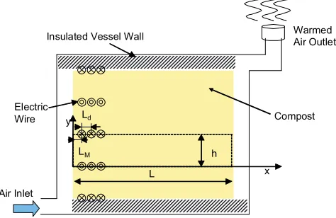
The problem to be considered in this study is schematically depicted in Fig. 1. Electric wires which generate the magnetic field are aligned in the compost with the interval of h in the vertical direction and with the interval of Ld in the horizontal direction. The first left electric wires are allocated in the compost with the distance of LM from the left inlet. The air flows into the compost from the left inlet and is warmed by exothermic heat of compost as it passes through the compost. And the warmed air flows up outside from the right exit. If the compost is deep enough, the airflow and the magnetic fields repeat themselves in successive cycles except the top and bottom. The airflow in porous medium is very slow. Therefore it could be assumed that there is no friction on the top and bottom wall. The solution domain, with the assumption of periodicity, is confined to a typical region bounded by the dashed line in Fig. 1. The airflow when the inlet pressure is equal to the exit pressure will be analyzed.

Frontiers in Heat and Mass Transfer

h L Air Inlet Warmed Air Outlet LM

Ld Compost

Electric Wire

Insulated Vessel Wall

y

x

Fig. 1Schematic Model of Compost Heating System (CHS)

2.2 Chemical Reactions

In compost process, microorganism dissolves easily degradable biomass and achieves living energy by metabolism activities. Compost process is complex system relating tremendous microorganism. The compost process can be divided into four phases based on ambient temperature: a mesophilic phase (phase I), a thermophilic phase (phase II), a cooling phase (phase III), and a maturation phase (phase IV). In phase I, the compost mass is at ambient temperature and may be slightly acidic. In phase II, the temperature exceeds 40 _°C, the mesophiles decline, and degradation is dominated by the thermophiles and Reaction I mainly occurs. As readily degradable substrates decline, heat loss exceeds metabolic heat generation and phase III, the cooling phase, is initiated and Reaction II mainly occurs. Phase IV, compost maturation, is critical to its agronomic use. An immature compost can introduce phytotoxic materials to the soil and Reaction III mainly occurs (Palmisano et al., 1996).

Reaction I: 1 2 2 2 2 2 4 H O H ) / y ( xCO O ) / z / y x ( O H C_{x y z}

Δ + + → − + + (1) Reaction II:

(

)

(

)

2 3 2 4 5 5 2 4 H O H ) / n )( y ( CO ) x ( n NO H C O ) / z / y x ( nNH O H C n _{x y z}

Δ + − + − + → − − + + + (2) Reaction III: 3 3 2 2 2 2 7 5 2 5 5 H nNH O nH nCO nO NO H C Δ + + + → + (3)

Glucose is chosen as a representative monosaccharide, the reaction in compost is expressed as

H CO O H O O H

C6 12 6 + 6 2 → 6 2 + 6 2 + Δ (4)

This reaction yields carbon dioxide of 1.38 kg and water vapor of 0.56 kg per oxygen of 1 kg. Air contains oxygen of 23% by mass and the rest being nitrogen and others. This nitrogen has nothing to do with these reactions. Therefore the constant density of air is assumed (Klejment et al., 2008).

2.3 Magnetizing Force

Gases are classified into paramagnetic or diamagnetic. Oxygen has paramagnetic property. Nitrogen, carbon dioxide, water vapor and argon gas have the diamagnetic property. The magnetic susceptibility of oxygen is positive and larger than those of other diamagnetic gases by two digits. Therefore, the magnetic force on diamagnetic gases is negligible. The magnetizing force f[N/m3_{], which acts on air of unit} volume, can be estimated from the mass fraction of oxygen ξO2 as

2 O O 0 P b χ ξ ρ M f 2 2   ∇

=₂ 1 (5)

where MP0= 4π×10-7 H/m，χO2=1.34×10-6 m3/kg (Weast et al., 1987).

Fresh air which flows into the compost, contains oxygen of 23 % by mass and is attracted toward magnetic field. However, the oxygen mass fraction continually decreases, as it passes through the compost because of microorganism metabolic reactions. The difference of oxygen mass fraction causes airflow in the compost, the details of which are discussed later.

2.4 Governing Equations

Steady, two-dimensional and laminar flow and constant properties are assumed. Darcy model is employed to represent the airflow through the porous medium compost. The governing equations for the airflow in the compost with magnetic field are follwing (Tagawa et al., 2002).

0 = ∂ ∂ + ∂ ∂ y v x u (6)         ∂ ∂ + ∂ ∂ − = x b χ ρξ 2M 1 x p μ K

u _{o o} 2

P0 2 2

 (7)         ∂ ∂ + ∂ ∂ −

= ρξ χ b_y

2M 1 y p μ K

v _{o o} 2

P0 2 2

 (8) ref , O O gl A 2 1 0 2 O 2 2 O 2 O O 2 2 3 2 2 2 2 ξ ξ ρ ρ A T 1 1 RT A exp A y ξ x ξ D y ξ v x ξ u ⋅ ⋅                   + ⋅       − ⋅ −         ∂ ∂ + ∂ ∂ ϕ = ∂ ∂ + ∂ ∂ (9)

where constants of the chemical reaction, A0, A1, A2 and A3 are

preexponential coefficient 1.495×107 _{mgO2/(kg h), energy of activation} 26.52 kJ/mol, temperature inhibition 67.2°C and shape factor 68 , respectively (Weppen, 2002).

The boundary conditions are following:

on x = 0 : u=u_in, v=0,

ξ

on y = 0 and h : =0

∂ ∂

y

u _{, 0}

=

v , =0

∂ ∂

y ξ_O2

on x = L : =0

∂ ∂

x u

, =0

∂ ∂

x v

, =0

∂ ∂

x ξ_O2

(10)

and also

out in p

DOI: 10.5098/hmt.v1.1.3005 ISSN: 2151-8629 Note that the uin is not known and its value will be obtained to satisfy

Eq. (11) by an arbitrary guess-and-correction iterative procedure.

2.5 Magnetic Flux Density

The magnetic flux density in a region is affected by electric wires locating far from the region. For calculation, the magnetic flux density in the region, it is necessary to take into consideration the effect of four wire rows both above and below the region. In this study, five electric wires are allocated with the distance Ld in the horizontal direction. When electric current direction changes alternately, the magnetic flux density is expressed by Biot-Savart's law as

( )

{

}

        

 

 _{− + −}

−

  

 

+

  

 

  

 

− + − −

=









= +

=

+

= =

j d

1)L (k L x 1) (

i d

l)h (4 y 1 2π

I M

2 kl

d M

5

1 k

1 l 8

1 l

2 kl 1 I 5

1 k 8

1 l P0

  

b

(12)

where I and dkl are electric current and distance from the electric wire, respectively. The difference between the alternately opposite direction of electric current and the same direction of electric current can be neglected (Tasaka et al., 2010). In this study, the case of the alternately opposite direction of electric current is calculated.

LM Ld

L h

y

x ~

‚ W

~ ‚ T A

B C

D

Fig. 2 Configuration of electric wires

Fig. 3 shows the contour plot of b2_{. This is the result for h = 0.2} m, Ld= 0.06 m, LM =0.05 m and I = 100 A. The b and b2 values at

distance of 0.005 m apart from one electric wire are 4.0×10-3 _{T and} 1.6×10-5 _T2_{, respectively. In this case, the distance of the electric wires} is wide enough to avoid interference of magnetic field among electric wires. In the magneto-aero-dynamics, the computational domain should be wider than the area where the magnetizing force affects on the fluid. If the computational domain is smaller than that area, the correct results will not be obtained. In this study, computation domain set larger than the area on which magnetic field have influence to meet this condition.

0 0.2 0.4 _X[m] 0.6 0.8 1 0

0.1 0.2

Y[

m

]

B2 1.33289E-05 1.02575E-05 7.18598E-06 4.11451E-06 1.04303E-06

Fig. 3 Contour plot of b2

3.

NUMERICAL PROCEDURE

The numerical methodology to solve the flow field is based on the SIMPLE method (Patankar, 1980). The SIMPLE method employs the finite volume method and discretes differential equations by integration in order to satisfy the conservation law of mass and momentum. The discretized procedure of the equations is based on the power law scheme of Patankar (1981), and the discretized equations are solved by using a line-by-line method. The pressure and velocity are linked by SIMPLE algorithm of Patankar (1980). The convergence criterion used in this computation was that the value of the mass flux residuals (mass flow) divided by the total mass flow in each control volume took a value under 10-13_{. The relaxation factors for the velocity and the} pressure were set to 10-2 _{and 0.1, respectively. About 9000 iterations} were required to obtain a converged solution. Almost all computations were performed with (52×22) grid points. These points are distributed in a uniform manner over the solution domain.

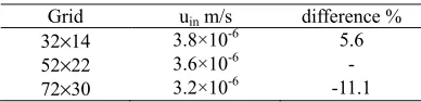
The grid size effect was confirmed on the case of L = 1.0 m, h = 0.2 m, the permeability K = 7×10-4 _m2_{, the porosity ϕ = 0.87 and the} particle density ρgl = 1820 kg/m3. Table 1 compares the inlet velocity

uin based on the case with x-directional number of grids × y-directional number of grids = 52_×22. The inlet velocity shows a tendency to decrease when the number of the grids increases. When the number of the grids increases from 32_×14 to 52_×22, the inlet velocity reduced from 3.8×10-6 _{m/s to 3.6×10}-6 _{m/s by 5.6 %. Similarly, when the} number of the grids increases from 52_×22 to 72_×30, the inlet velocity decreases from 3.6×10-6 _{to 3.2×10}-6 _{m/s by 11.1%. The grid size effect} on the inlet velocity of this problem is relatively large. However, the computations are mainly performed with x-directional number of grids

× y-directional number of grids = 52×22.

Table 1 Effect of grid size on inlet velocity

Grid uin m/s difference %

32×14 3.8×10-6 _5.6

52_×22 3.6×10-6 _-

72×30 3.2×10-6 _-11.1

4.

RESULTS AND DISCUSSIONS

The range of the geometrical parameters are listed in Table 2. The compost length, L, is fixed at one meter for all computations. The compost size in this study is considerably small, comparing to a full-scale windrow size compost. It is complex and high costly to research the natural large compost in the real world. Therefore it is very useful to analyze the available data of a bench-scale size compost and develop future commercial-size model.

The computations were performed for the case of cow manure. The Kozeny-Carman constant of cow manure with its water content of 73.7% is 3532 (1/m2_{) (Das et al. 1997). Then, the air permeability of} the cow manure with its porosity of 0.9 (its free air space of 0.9) is 2.06×10-2 _m2 _{by calculating from the Kozeney-Carman equation. All} computations were performed for the case of K = 2.06×10-2 _m2 _{and the} particle density, ρgl = 1381 kg/m3. The diffusion coefficient of oxygen,

nitrogen and carbon dioxide in the air are 1.78×10-5_{, 1.34×10}-5 _and 1.37×10-5 _m2_{/s, respectively (Weast et al. 1987). However, in this} analysis, an identical diffusion coefficient is assumed. The value of 1.78×10-5 _m2_{/s was chosen for all computations because magnetizing} force acts on only oxygen.

Table 2 Geometric parameters

Range (m) Typical length (m)

L - 1

h 0.04 ∼ 0.4 0.2

Ld 0.02 ∼ 0.12 0.06

LM 0.03 ∼ 0.1 0.05

4.1 Velocity Vectors, Mass Fraction & Pressure Contours

Fig. 4 shows the typical case of 100A current. In the magneto-aero-dynamics, not only the gradient of square magnetic flux density but also the gradient of concentration drives airflow by magnetic field. In Fig. 4(b), the concentration of oxygen changes dramatically in the area from x = 0 to 0.3m. Therefore, electric wires are set up at only the area which the surge gradient of the concentration can be observed. The airflow is accelerated by the magnetizing force in the area from x = 0 to 0.3m.

0 0.2 0.4 0.6 0.8 1

X[m]

0 0.1 0.2

Y[

m

]

0.005[m/s]

(a)

0 0.2 0.4 0.6 0.8 1

X[m]

0 0.1 0.2

Y[

m

]

OMF 0.187126 0.144252 0.101378 0.0585044 0.0156305

(b)

0 0.2 0.4 0.6 0.8 1

X[m]

0 0.1 0.2

Y[

m

]

P 1.84241E-06 1.41655E-06 9.90692E-07 5.6483E-07 1.38969E-07

(c)

Fig. 4 (a) Velocity vectors and contour plots of (b) mass fraction of oxygen and (c) pressure for the typical case

4.2 Flow by Pressure Difference

For information, the computation was also performed for the typical case without magnetic field. This is, the flow is induced by the pressure difference at the inlet and the outlet. In the case of the magnet induced flow (the case of Fig. 4), the inlet velocity, uin is 8.9×10-5 m/s. To make the identical inlet velocity, the pressure difference of 6.8×10-8 Pa is given. The inlet pressure and the exit pressure are 6.2×10-12 _and -6.8×10-8 _{Pa. Note that pin and pout are the average pressures at the} innlet and outlet, respectively. Fig. 5 (a) shows the velocity vectors of the airflow induced by the pressure difference. The circulation in Fig. 4(a) can not be seen in the airlow induced by the pressure difference. Fig. 5 (b) shows the contour of oxygen mass fraction. Fig. 5 (c) shows the contour of pressure. The pressure gradually decreses along the compost. To induce the airflow with the same velocity without

magnetic field, such a pressure difference of 6.8×10-8 _{Pa is required by} some mechanical drive during a considerable long time of fermentation.

0 0.2 0.4 _X[m] 0.6 0.8 1 0

0.1 0.2

Y[

m

] 0.0005[m/s]

(a)

0 0.2 0.4 _X[m] 0.6 0.8 1 0

0.1 0.2

Y[

m

]

OMF 0.187076 0.144152 0.101228 0.0583046 0.0153807

(b)

0 0.2 0.4 _X[m] 0.6 0.8 1 0

0.1 0.2

Y[

m

]

P -1.27638E-08 -2.55356E-08 -3.83075E-08 -5.10793E-08 -6.38512E-08

(c)

Fig. 5 (a) Velocity vectors and contour plots of (b) mass fraction of oxygen and (c) pressure for the typical case without electric current

-0.0004 -0.0002 0 0.0002 0.0004

∂

b

2 /∂

x (

T

2 m -1 )

(a)

-1 -0.5 0

∂

ξO2

/

∂

x

(b)

0 0.2 0.4 0.6 0.8 1

0 0.0005 0.001 0.0015

x (m)

u (m

s

-1 )

(c)

Fig. 6 correlation among u, ∂b2/∂xand _∂ξ /_∂x

2

DOI: 10.5098/hmt.v1.1.3005 ISSN: 2151-8629

4.3 Correlation among

u

,

and

Fig. 6 shows the effect of ∂b2/∂xand ∂ξO2/∂x on the Darcy velocity u on the line of y = 0.005 m. The u is accelerated when _∂b2/_∂x is positive. On the other hand, the u is decelerated when ∂b2/∂x is negative. As seen in Fig. 6(a), the ∂b2/∂x oscillates at the area where the electric wires are allocated. The magnetizing force is expressed by product of the ∂b2/∂x and ∂ξO2/∂x . Therefore, the amount of acceleration is considerably large near the inlet due to the larger gradient of concentration.

4.4 Effect of Electric Current on Inlet Velocity, u

The computations were also performed to investigate the effect of electric current on inlet velocity uin. The currentranges from 10 to 100 A. The results are shown in Fig. 7. These are the results for the typical case only the exception of the electric current. The inlet velocity increases exponentially with increases in the current. According to the tendency in Fig. 7, larger current is desirable for larger magnetic field which induces faster flow to supply sufficient oxygen. In this study, the case of the current 100A are calculated.

0 20 40 60 80 100

0 2 4 6 8 10

×10-5]

I (A)

uin

(m

s

-1 )

Fig. 7 Inlet velocity as a function of electric current

0 0.1 0.2 0.3 0.4

0 1 2 3 4 [×10-4_]

h (m)

uin

(m

s

-1

)

Fig. 8 Inlet velocity as a function of h

4.5 Effect of Vertical Distance of Electric Wires, h on Inlet

Velocity, u

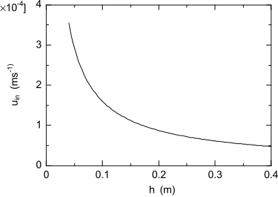
The computations were also performed to investigate the effect of vertical distance of electric wires, h on inlet velocity, uin. The vertical distance of electric wiresranges from 0.04 to 0.4 m. The results are shown in Fig. 8. These are the results for the typical case only the

exception of the vertical distance of the electric wires, h. The thickness of velocity acceleration in y-direction is almost constant regardless of h.

When h is small, the thickness of velocity acceleration accounts for a larger percentage in y-direction. That is why uin decreases exponentially when h increases.

4.6 Effect of Horizontal Distance of Electric Wires, L

on

Inlet Velocity, u

The computations were also performed to investigate the effect of horizontal distance of electric wires, Ld on inlet velocity, uin. The horizontal distance of electric wires ranges from 0.02 to 0.12 m. The results are shown in Fig. 9. These are the results for the typical case only the exception of the horizontal distance of the electric wires, Ld. When the horizontal distance is below 0.06 m, the interference of magnetic fields among wires cannot be avoided. It results in the decrease of acceleration distance which causes reduced inlet velocity. On the other hand, when the horizontal distance between wires is above 0.06, the end of intense magnetic field would be put out of the concentration gradient. Therefore the intense magnetic flux density cannot contribute to the acceleration of velocity and the inlet velocity is reduced. Judging from Fig. 9, the optimum Ld is 0.06m.

0 0.05 0.1

0 2 4 6 8 10 [×10-5]

Ld (m) uin

(ms

-1 )

Fig. 9 Inlet velocity as a function of Ld

4.7 Effect of Distance from Inlet to First Electric Wire, L

on Inlet Velocity, u

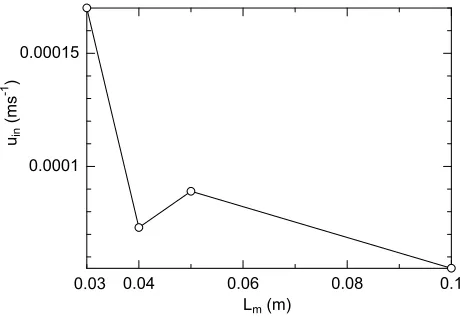
The computations were also performed to investigate the effect of the distance from the inlet to the first electric wire, Lm on inlet velocity, uin. The distance from the inlet to the first electric wire ranges 0.03 to 0.1 m. The horizontal distance of electric wires is constant, optimum value of 0.06 m. The results are shown in Fig. 10. These are the results for the typical case only the exception of Lm. When the first electric wire is closer to the inlet, the larger inlet velocity is obtained. On the other hand, the first electric wire goes away from the inlet, the end of the intense magnetic flux denstiy is located at the area which the gradient of the concentration does not exit. Therefore the intense magnetic flux density cannot contribute to the acceleration of velocity and the inlet velocity is reduced. Judging from Fig. 10, the optimum Lm is 0.03 m in this calculation.

0.04 0.06 0.08 0.1 0.0001

0.00015

Lm (m) uin

(ms

-1 )

0.03

Fig. 10 Inlet velocity as a function of Lm

5.

CONCLUSIONS

Airflow through porous medium compost induced by electric wires has been investigated numerically. The computations were performed for cow manure. The following conclusions are obtained:

1. The utilization of electric wires is effective to improve aeration in compost.

2. The maximum inlet velocity uin, 6.5×10-4 _{m/s is obtained when the} vertical distance of electric wires, the horizontal distance of electric wires and the distance from the inlet to the first electric wire are the optimum values, 0.04, 0.06 and 0.03 m, respectively.

NOMENCLATURE

A0 preexponential coefficient (mgO2/(kg h)) A1 energy of activation (kJ/mol)

A2 temperature inhibition (°C) A3 shape factor

b magnetic flux density vector (T = Wb/m2 _{= kg s}-2 _A-1₎ D diffusion coefficient (m2_/s)

d distance from wires (m) L compost length (m)

LM distance from the inlet to the first wire(m)

Ld horizontal distance of wires (m)

f magnetizing force per unit volume (N/m3₎ h vertical distance of wires (m)

ΔH exothermic reaction energy (J/kg)

I electric current (A)

MP0 vacuum magnetic permeability (H/m = m kg s-2 _A-1₎

p pressure (Pa)

uin inlet velocity (m/s) u, v velocity components (m/s) x, y coordinates (m)

Greek Symbols

χ magnetic susceptibility of unit mass (m3_/kg)

ϕ porosity

μ viscosity (Pa s)

ρ density (kg/m3₎

ξ mass fraction

Subscripts

gl compost material, glucose in inlet

out outlet o2 oxygen

ref reference

REFERENCES

Agnew, J.M., and Leonard, J.J., 2003, "The Physical Properties of Compost", Compost Science & Utilization, 11,3, pp238-264.

Alexander M., 1994, “Biodegradation and Bioremediation”, Academic Press.

Das, K., and Keener, H.M., 1997, "Moisture effect on compaction and permeability in composts", J. Environmental Engineering, 123(3), pp. 275-281

DOI: 10.1061/(ASCE)0733-9372(1997)123:3(275)

Klejment, E., et. al., 2008, “Testing of thermal properties of compost from municipal waste with a view to using it a renewable, low temperature heat source”, Bioresource Technology, 99, pp. 8850-8855. DOI: 10.1016/j.biortech.2008.04.053

Lynch, N.J., Cherry, R.S., 1996, "Design of passively aerated compost piles: vertical air velocities between the pipes, Biotechnology Progress, 12, pp. 624-629

DOI: 10.1021/bp960048+

Nield, D.A., and Bejan, A.,1992, Convection in Porous Media, Springer-Verlag, New York

Palmisano, A.C.,and Barlaz, M.A., 1996, Microbiology of Solid Waste, CRC Press Inc.

Patankar, S.V., 1980, Numerical Heat Transfer and Fluid Flow, Hemisphere Publishing Co., Washington, D.C.

Patankar, S.V., 1981, “A Calculation Procedure for Two-Dimensional Elliptic Situations”, Numerical Heat Transfer, 4, pp. 409-425.

DOI: 10.1080/01495728108961801

Tagawa, T., Shigematsu, R., and Ozoe, H., 2002, “Magnetizing force modeled and numerically solved for natural convection of air in a cubic enclosure: effect of the direction of the magnetic field”, Int. Journal of Heat and Mass Transfer, 45, pp. 267-277.

DOI: 10.1016/S0017-9310(01)00149-1

Tasaka, E, et al., 2010, “Enhancement of Oxygen Diffusion in a Gas Diffusion Layer of a Fuel Cell Electrode by Magnetizing force”, IMECE2010-39428, to be submitted.

Weast, R.C., et. al., 1987, CRC Handbook of Chemistry and Physics, CRC Press Inc.