INTELIGENCIA ARTIFICIAL
http://journal.iberamia.org/
Fuzzy Neural Networks based on Fuzzy Logic
Neurons Regularized by Resampling Techniques and
Regularization Theory for Regression Problems
Paulo Vitor de Campos Souza
1,2, Augusto Junio Guimar˜
aes
2, Vanessa Souza Ara´
ujo
2,
Thiago Silva Rezende
2, Vinicius Jonathan Silva Ara´
ujo
21Federal Center for Technological Education of Minas Gerais, Faculty UNA of Betim,
Minas Gerais Brazil.
[email protected], [email protected]
2
Faculty UNA of Betim Minas Gerais, Brazil
[email protected], [email protected], [email protected],[email protected]
Abstract This paper presents a novel learning algorithm for fuzzy logic neuron based on neural networks and fuzzy systems able to generate accurate and transparent models. The learning algorithm is based on ideas from Extreme Learning Machine, to achieve a low time complexity, and regularization theory, resulting in sparse and accurate models. A compact set of incomplete fuzzy rules can be extracted from the resulting network topology. Experiments considering regression problems are detailed. Results suggest the proposed approach as a promising alternative for pattern recognition with good accuracy and some level of interpretability, in addition to a more compact network architecture to work with regression problems.
Keywords: Bootstrap Lasso, Extreme Learning Machine, Fuzzy Logic Neurons, Fuzzy Neural Networks, Regres-sion Problems.
1
Introduction
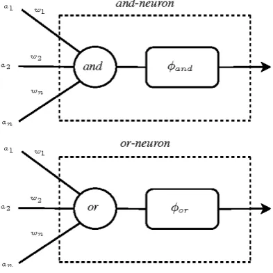
Fuzzy neural networks are networks based on fuzzy logic neurons [50]. These models are a synergy between fuzzy sets theory, as a mechanism for knowledge representation and information compaction, and neural networks. The main feature of these models is transparency since a set of fuzzy rules can be extracted from the network structure after training [10]. Thus, the neural network is now seen as a linguistic system, preserving the learning capacity of ANN. Its fuzzy neurons are composed of triangular norms, which generalize the union and intersection operations of classical clusters to the theory of fuzzy sets. Furthermore, these models have a neural network topology which enables the utilization of a large variety of existing machine learning algorithms for structure identification and parameter estimation. Fuzzy neural networks have already been used to solve several distinct problems including pattern classification [10] and [60], time series prediction [4] [27] [8] and dynamic system modeling [26] [19] [41] [42]. Examples of fuzzy neurons are and and or neurons [54]. These logic based neurons are nonlinear mappings of the form [0, 1]N → [0, 1], where N is the number of inputs. The processing of these neurons is performed in two steps. Firstly, the input signals are individually combined with connection weights. Next, an overall aggregation operation is performed over the results obtained in the first step and and or neurons use t-norms and s-norms (t-conorms) to performed output processing. Several learning algorithms for fuzzy neural networks have already been proposed in the literature. Usually, learning is performed in two steps. Firstly, the network topology is defined. This step involves defining fuzzy sets for each input variable, selecting a suitable number
ISSN: 1137-3601 (print), 1988-3064 (on-line) c
of neurons and defining network connections. The most commonly used methods for structure definition are clustering [10], [4], [8], [26], [41], [42] and evolutionary optimization [51] [52] [43]. Once the network structure is defined, free parameters are estimated. A number of distinct methods have already been used in this step including reinforcement learning [10], [4], [26], gradient-based methods [52], [53], genetic algorithms [41], least squares [8], [42] and hybrid strategy [60] through a grid partition of the data (without grouping) [37]. Regarding network structure optimization, the two most commonly used methods may present significant deficiencies. Clustering has a low computational cost when compared with evolutionary optimization. Nevertheless, interpretable fuzzy rules usually canˆat be extracted from the resulting network, since fuzzy sets generated by clustering are typically challenging to be interpreted [21]. Evolutionary optimization based methods may be able to generate interpretable fuzzy rules. However, they have a high computational complexity. This paper proposes a novel learning algorithm for fuzzy neural networks able to generate compact and accurate models. The learning is performed using ideas from Extreme Learning Machine [34], to speed-up parameter tuning, and regularization theory [18]. First, fuzzy sets are generated for each input variable. Next, a large number of candidate fuzzy neurons are created with randomly assigned weights. In this step, only a random fraction of the input variables are used in each candidate neuron. Following, the bootstrap Lasso algorithm [3] is used to define the network topology by selecting a subset of the candidate neurons. Finally, the remaining network parameters are estimated through least squares. The resulting network is a sparse model and can be expressed as a compact set of incomplete fuzzy rules, that is, rules with antecedents defined using only a fraction of the available input variables [21]. A similar approach was used for classification problems [60], but taking advantage of the universal approximation capability of ELM [36], the model was adapted to perform resolutions for regression problems. The paper is organized as follows. Next section reviews the necessary fundamental concepts about fuzzy logic neurons and fuzzy neural networks. Section III details the proposed new learning algorithm able to generate small and transparent networks. Section IV presents the experimental results for regression problems and comparison with alternative classifiers. Finally, the conclusions and further developments are summarized in section V.
2
Fuzzy Neural Networks
2.1
Neural Networks
A neural network is a distributed, and parallel processor made up of less complicated processing units, in order to store knowledge about a theme or a set of characteristics, making it available for use in similar tasks human beings [25]. Already [9] complements that the neural network can be connected entirely where each neuron is connected to all the neurons of the next layer, partially connected where each neuron is, or locally connected where there is a partial connection oriented for each type of functionality. To perform the training of a neural network requires a set of data that contains patterns for training and desired outputs. As artificial neural networks seek to simulate the behavior of the human brain, knowledge is acquired by the network through the environment that surrounds it, through a learning process. Already in the storage of knowledge, the analogy is made with the forces of connections between the neurons, known as synaptic weights.
2.2
Fuzzy Systems
The fuzzy systems are based on fuzzy logic, developed by [62]. His work was motivated by a wide variety of vague and uncertain information in human decision making. Some problems cannot be solved with standard Boolean logic. The fuzzy model’s systems can be divided into three main concepts [28]:
-Fuzzy Linguistic Models; -Relational Fuzzy Models; -Functional Fuzzy Models.
The fuzzy linguistic models are those that use a rule base if-then and an inference method for relating inputs and outputs. This model is called linguistic to make direct use of the linguistic representation of rules [28]. In turn, the nebulous relational models, as the name itself says, represent the mapping between the fuzzy sets of input and output through nebulous relations [54]. Moreover, finally, the fuzzy functional models (Takagi-Sugeno) are models with terms in the antecedent of a rule and a function of the entrances in the consequent.
2.3
Fuzzy logic Neurons
Fuzzy logic neurons are functional units able to perform multivariate nonlinear operations in unit hypercube [0, 1]N [0, 1] [50], whereN is the number of inputs. The term logic is associated with the logic disjunction or and
conjunction and operations performed by these neurons using, in this work, t-norms and s-norms. The or and
w= [w1, w2, ..., wN], where aj ∈[0, 1] andwj∈ [0, 1] forj = 1, ... ,N, and subsequently globally aggregating
these results. They were initially defined as follows [50]:
h=AN D(a;w) =Tin=1(aiswi) (1)
h=OR(a;w) =Sin=1(aitwi) (2)
whereS ands are s-norm and T and are t-norm.
The or-neuron is interpreted as a logical expression that performs an and-type local aggregation of the inputs and the weights using a t-norm, followed by an or-type global aggregation of the results using as s-norm. The and-neuron is interpreted similarly, with an or-type local aggregation and an and-type global aggregation. Figure 1 illustrates the neurons, as defined in [50].
Figure 1: Fuzzy Logic Neurons.
The activation functionsφand andφor can, in general, be nonlinear mappings. In this paperφand (ε) =φor (ε) =ε, i.e., they are defined as the identity function. According to [51], the local aggregations performed by these neurons can be interpreted as weighting operations of the inputs, since the role of the weights is to differentiate among distinct levels of impact that individual inputs might have on the global aggregation result. In the case of the or-neuron, lower values of wj reduces the impact of the corresponding input, while higher values do not affect the original value of the corresponding input. In limit, if all weights are set to 1, the neuron output is a plain or combination of the inputs. For the and-neuron, the interpretation of the weightˆas values is inverse, i.e., higher values ofwjreduces the impact of the corresponding input. For this neuron, in the limit, if all weights are set to
0, the output is a plain and combination of the inputs. In order to unify the interpretation of the weights for the and and or neurons, (i.e., a low value of w reduces the impact of the associated input) the and-neuron used in this paper is defined as:
h=AN D(a;w) =Tin=1(ais(1−w)i) (3)
2.4
Fuzzy Neural Networks concepts
2.4.1 Characteristics of Fuzzy Neural Networks
Fuzzy neural networks can be classified concerning how their neurons are connected. This form of connection sets as the signals will be transmitted on the network. In general, there is the feedforward where fuzzy neurons are grouped into layers and the signal across the network in a single direction, usually the model until your output generating an expected result. Fuzzy neurons in the same layer that have no connection and its networks are also known as no feedback networks [24]. This type of connection is the most common among the models of fuzzy neural networks [8], [41] and [42]. Finally, there are the networks that are used with feedback, also called recurring (recurrent). In this type of fuzzy network, neurons are also assembled in layers, but there is information power in neurons in the same layer, and it may even happen to own fuzzy neuron in question, or even previous layers, if former. Figure 2 shows plainly the difference between a recurrent network and a forward network.
Figure 2: Example of networks feedforward and networks recurrent. [49]
The number of layers is also a factor that can differentiate fuzzy neural networks. In the models, each layer is responsible for a specific task or function. In general, the first layer is responsible for dealing with and the last inputs for bringing the network response. Between these two layers, there are other intermediates, that can be hidden or not. Depending on the model and what he proposes, each layer has a specific function. Examples of the fuzzy neural networks that have three layers in some models the first two are based on concepts of fuzzy systems and the third is an artificial neural network. The models of [26], [41] and [12] using fuzzy neurons (unineurons) to aggregate the values of the first layer. When we evaluate the networks on the types of neurons that compose their layers, we can highlight the models that have fuzzy neurons and/or type. These models generally use these structures to use operators of t-norm and s-norms. As an example of fuzzy neural networks that use these types of neuron the models [60], [55], [38] and [14]. Evaluating the type of fuzzy neural networks training can highlight that these algorithms are a set of well-defined rules for resolving learning problems. These methodologies are seeking training, in General, to simulate human learning to learn or refresh their new concepts, working mainly in network factors, for example, the values of the synaptic weights. In General, both for artificial neural networks and fuzzy neural networks learning can be classified according to the following paradigms:
-Supervised-when using some external factor that indicates to the network which is the desired result to the problem in question.
-Unsupervised-when no external agent is indicating the network response input standards submitted to the models.
-Strengthening-when an external evaluator unit measures the response of the model [24].
the fuzzy neural networks also have featured, because the way they act reflects directly on the variables involved in the model. The method with which the entries are handled can set parameters such as activation functions, membership functions of fuzzy sets, network topology, among others [41]. Fuzzy neural networks can use grouping methods, such as the c-means clustering and your fuzzy version: fuzzy c-means [15], [5], density-based methods of data (clouds) [2], online group (eClustering [1]), the ePL [44], F-scores [13], and ANFIS approach [60], [12] and [14], [11] among others.
2.5
Fuzzy Neural Networks architecture proposes
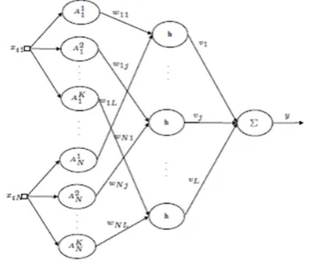
The fuzzy logic neurons described in the previous section can be used to construct fuzzy neural networks and solve pattern recognition problems. Figure 3 illustrates the feed-forward topology of the fuzzy neural networks considered in this paper.
Figure 3: Feedforward fuzzy neural network
The first layer is composed of neurons whose activation functions are membership functions of fuzzy sets defined for the input variables. For each input variable xij, K fuzzy sets are defined Ak, k = 1... K whose
membership functions are the activation functions of the corresponding neurons. Thus, the outputs of the first layer are the membership degrees associated with the input values, i.e.,aj k=µAk. forj = 1...,N andk = 1, ...
,K, whereN is the number of inputs andK is the number of the membership functions of each input. For this, the ANFIS algorithm [37] is used.All the neurons of the first layer are of the Gaussian type, formed through the centers obtained by the functions of Gaussian pertinence and with the value of sigma defined in a random way.
The second layer is composed ofLfuzzy logic neurons. Each neuron performs a weighted aggregation of some of the first layer outputs. This aggregation is performed using the weightswil (fori = 1... N and l = 1... L).
For each input variablej, only one first layer outputakj is defined as the input of thel-th neuron. Furthermore,
in favor of generating sparse topologies, each second layer neuron is associated with onlynl ≤N input variables, that is, the weight matrixwis sparse. Finally, the output layer uses a classic linear perceptron neuron to compute the network output:
y=
L
X
j=0
hlvl (4)
wherehlforl= 1, ... ,Lare the outputs of second layer neurons,vlare the output layer weights andh0= 1.
As discussed, incomplete fuzzy rules can be extracted from the network topology. Figure 4 illustrates an example of a fuzzy network composed by and-neurons. This network has 2 input variables, 2 membership functions for each variable and 3 neurons, i.e.,M = 2,K = 2 andL= 3. The following if-then rules can be extracted from the network structure:
Rule1: Ifxi1 isA11 with certaintyw11...
andxi2 isA12 with certaintyw21...
Theny1isv1
Rule2: Ifxi1 isA21 with certaintyw12...
Rule3: Ifxi2 isA22with certaintyw23...
Theny3 isv3(5)
where each free parametervlforl = 1, ..., 3 can be interpreted as a singleton.
Figure 4: Example of a fuzzy neural network
3
Fuzzy Neural Networks Training Algorithm
The learning algorithm detailed in [41] for fuzzy neural networks uses clustering for topology definition and genetic algorithms for parameter tuning. This learning procedure can generate accurate models. However, the resulting network is usually not interpretable, since the fuzzy sets for each input variable are defined using clustering [21]. Furthermore, the learning algorithm has a high time complexity, given the nature of the parameter tuning algorithm.
In [42] the genetic algorithm is replaced by a new parameter tuning procedure based on ideas from ELM. Extreme Learning Machine [36] is a learning algorithm developed initially for single hidden layer feed-forward neural networks (SLFNs). The algorithm assigns random values for the first layer weights and analytically estimates the output layer weights. When compared with traditional methods for SLFNs learning, this algorithm has good generalization performance and shallow time complexity, since only the output layer parameters are tuned [35]. It has been proved that SLFNs trained using this approach have a universal approximation property, for a Fig. 5. Input domain partition using five triangular membership functions given a choice of the hidden nodes [34].
Inspired by this SLFN learning scheme, a new fast learning algorithm for fuzzy neural networks is described in [42]. This approach assigns random values for the neuron parameters and estimates the parameters of the output layer neuron using least squares. This learning algorithm has a low computational cost, but still generates networks which are not easily interpretable, since the fuzzy sets are still defined using clustering.
This paper proposes an improvement in the learning algorithm described in [42] implemented in [60] in order to improve the interpretability of the resulting networks for regression problems. A variable selection algorithm based on regularization theory is used to define the network topology. This algorithm can generate a sparse topology which can be interpreted as a compact set of incomplete fuzzy rules. The proposed learning algorithm initially defines first layer neurons by dividing each input variable domain interval intoK fuzzy sets [37], whereK
is usually a small number. Next,Lccandidate neurons are randomly selected from theLneurons, whereLc≤L.
If Lc chosen is greater than L, all L neurons created are considered as Lc. Usually Lc is initialized with 200
like [60]. For each candidate neuron l = 1... Lc, first, a random fraction of the input variables are selected. A
random valuenlis sampled from a discrete uniform distribution defined over the interval [1, N]. The value nl
represents the number of input variables associated with thel-th neuron. Next,nlinput variables are randomly
selected. For each input variable is chosen, a random fuzzy set (first layer neuron) is selected as the input of thel-th neuron and the corresponding weightwj l is sampled from a uniform distribution over the interval [0, 1].
One must note that, after this step, for each neuronl, onlynlweightswj l will have nonzero values, i.e., only the
cost function. The approach of [60] was also used for the model that will act on linear regression problems. The learning algorithm assumes that the output of a network composed by allLsselected neurons can be written as
[60]:
f(xi) = Ls
X
i=0
vihi(xi) =h(xi)v (6)
wherev= [v0, v1, v2, ..., vLc]T is the weight vector of the output layer andh(xi) = [z0, z1(xi), z2(xi)ˆazLI¨(xi)
] is the augmented output (row) vector of the second layer, forz0= 1. In this context,h(xi) is considered as the
non-linear mapping of the input space for a space of fuzzy characteristics of dimension Ls.
Note that Equation (6) can be seen as a simple linear regression model since the weights connecting the first two layers are randomly assigned and the only parameters left to be estimated the weights of the output layer. According to ELM learning theory [36], a general type of feature mappings h (xi) can be used in ELM. This theory says so ELM can approximate any continuous target functions (Universal Approximation Capability [33] and [32] for details). What this feature allows the ELM can be used for regression problems [31]. A learning machine with a feature mapping which does not satisfy the universal approximation condition cannot approximate all continuous target functions. Thus, the universal approximation condition is not only a sufficient condition but also a necessary condition for a feature mapping to be widely used [31]. Thus, the problem of selecting the best candidate neurons subset can be seen as an ordinary linear regression model selection problem [17]. One commonly used approach for model selection is the Least Angle Regression (LARS) algorithm [16]. The LARS is a regression algorithm for high-dimensional data which can estimate not only the regression coefficients but also a subset of candidate regressors to be included in the final model. Given a set ofD distinct observations (xi, yi),
wherexi =[xi1, xi2, ..., xiN]T ∈RN andyi∈Rfori = 1, ... ,D, the cost function of this regression algorithm is
defined as:
D
X
i=1
kh(xi)v−yik.2+λkvk.1 (7)
whereλ is a regularization parameter, commonly estimated by cross-validation andkvkis a weight norm. The first term of (7) corresponds to the sum of the squares of the residues (RSS). This term decreases as the training error decreases. The second term is an L1 regularization term. This term is used for two reasons. First, it
improves the network generalization, avoiding over fitting [18]. Second, it can be used to generate sparse models [57]. In order to understand why LARS can be used as a variable selection algorithm, Equation (7) is rewritten as: [16].
min
β RSS(v)
s.t. ||v||1≤β
(8)
whereβis an upper-bound on theL1-norm of the weights. A small value ofβ corresponds to a high value ofλ,
and vice versa. This equation is known as least absolute shrinkage and selection operator [22], or lasso. As in the ridge regression [30], we can re-parameterize the constantβ0, standardizing the predictors. Comparing with the
ridge regression, we can say that it replaces the penalty termβj2 withkβjk. This constraint makes the solution
nonlinear as a function ofyi, not obtaining a complete expression for the calculation of the coefficients as in the
ridge regression [23]. βcan be calculated by:
βlasso= arg min β
n
X
i=1
(yi−β0−
p
X
j=1
xijβj)2 (9)
subject
N
X
i=1
|βj| ≤t (10)
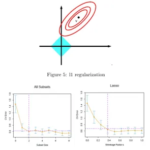
Figure 5 illustrates the contours of the RSS objective function, as well as thel1 constraint surface. It is well
known from the theory of constrained optimization that the optimum solution corresponds to the point where the lowest level of the objective function intersects the constraint surface. Thus, one should note that, whenβgrows until it meets the objective function, the points in the corners of thel1surface (i.e., the points on the coordinate
axes) are more likely to intersect the RSS ellipse than one of the sides [57]. Figure 5 shows the estimated prediction error curves and the standard error for the lasso method for the example of an any synthetic database.
.
Figure 5: l1 regularization
Figure 6: Estimated prediction error curves and their standard errors for the lasso regression method according to subset size [17].
The LARS algorithm can be used to perform model selection since for a given value ofλonly a fraction (or none) of the regressors have corresponding non-zero weights. If λ= 0, the regression problem becomes unconstrained, and all weights are non-zero. As λ increases from 0 to a specific λmax value, the number of non-zero weights
decreases fromN to 0. For the problem considered in this paper, the regressorshlare the outputs of the candidate neurons. Thus, the LARS algorithm can be used to select an optimum subset of the candidate neurons which minimizes (7) for a given value of λ, selected using cross-validation. One must note that this is not a novel approach and has already been used for SLFN pruning [56], [46] and fuzzy model identification [56]. However, one disadvantage of using the LARS algorithm for model selection is that it can give entirely different results for small perturbations in the dataset [57]. If this algorithm is executed for two distinct noisy datasets drawn from the same problem very distinct network topologies may be selected, compromising model interpretability. One existing approach to increase the stability of this model selection algorithm is to use bootstrap resampling. The LARS algorithm is executed on several bootstrap replicates of the training dataset. For each replicate considered, a distinct subset of the regressors is selected. The regressors to be included in the final model are defined according to how often each one of them is selected across different trials. A consensus threshold is defined, sayγ = 80%, and a regressor is included if it is selected in at least 80% of the trials. This algorithm is known as bootstrap lasso [3]. In this paper, the bootstrap lasso algorithm is used for topology definition.
to an exponentially fast withn, while it selects all other variables with strictly positive probability. This new methodology can select the variables most relevant to the model by discarding the least essential variables. When using resampling methods such as the bootstrap, it is possible to imitate the availability of several datasets even if it is using a single data set. Using the bootstrap concept and realizing the intersection between supports. Bach [3] developed a consistent estimating model of regularization, without the conditions of consistencies required by the lasso method. To this new procedure, it gave the name of Bolasso (bootstrap-enhanced least absolute shrinkage operator). This new framework can be seen as a voting scheme applied to the supports of lasso method estimates. However, Bolasso can be seen as a regime of consensus combinations where the most significant subset of variables on which all regressors agree when the aspect is the selection of variables is maintained. [3]. Bolasso procedure is summarized in Algorithm 1.
Algorithm 1:Bolasso- bootstrap-enhanced least absolute shrinkage operator (b1) Letnbe the number of examples, (lines) in X:
(b2) Shownexamples of (X, Y), uniformly and with substitution, called here (Xsamp,Y samp). (b3) Determine which weights are nonzero given aλvalue.
(b4) Repeat steps b1: b3 for a specified number of bootstrapsb.
(b5) Take the intersection of the non-zero weights indexes of all bootstrap replications. Select the resulting variables.
(b6) Revise using the variables selected via non-regularized least squares regression (if requested). (b7) Repeat the procedure for each value ofbbootstraps and λ(actually done more efficiently by
collecting interim results).
(b8) Determine optimal values for λandb.
Finally, once the network structure is defined, the learning algorithm has only to estimate the output layer vectorv = [v0, v1, v2...vL]T which best fits the desired outputs. In this paper these parameters are computed
using the Moore- Penrose pseudo-inverse [20]:
v= (HTH)−1HTY =H+Y (11) where H is defined as:
H =
h0 h1(x1) ... hL(x1)
h0 h1(x2) ... hL(x2))
h0 h1(xN) ... hL(xN))
N×k
(12)
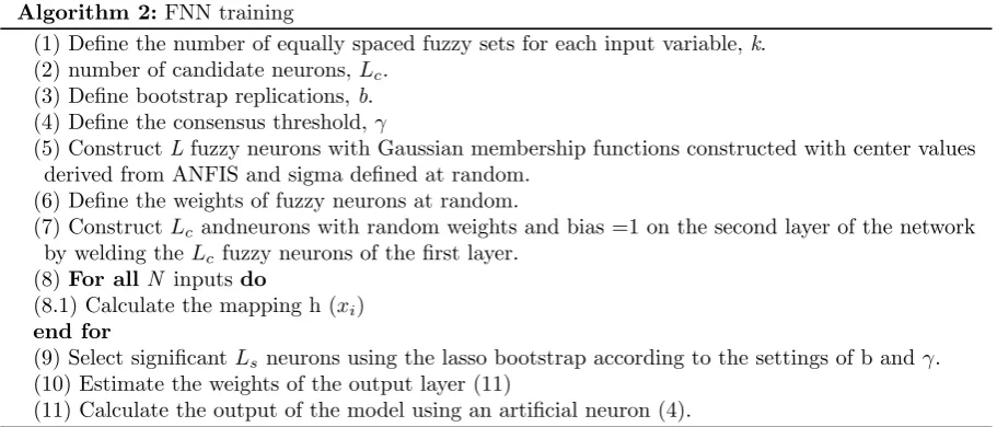
The learning procedure is summarized in Algorithm 2. The algorithm has four parameters: - the number of membership function,K;
- the number of candidate neurons,Lc;
- the number of bootstrap replications,b; - the consensus threshold,γ.
4
Experiments
The fuzzy neural network learning algorithm described in the previous section is evaluated using regression problems. For all experiments in this section, only networks composed by neurons are considered. All and-neurons use the product (t-norm) and the probabilistic sum (s-norm) and only Gaussian membership functions are used. The network used in the experiments was named R-ANDNET. In all tests the valueK= 3 andLc=200
like [60].
The accuracy of the R-ANDNET is evaluated for benchmark regression problems. To perform the comparison between the proposed models in this paper, algorithms were chosen to make two comparisons.
Algorithm 2: FNN training
(1) Define the number of equally spaced fuzzy sets for each input variable,k. (2) number of candidate neurons,Lc.
(3) Define bootstrap replications,b. (4) Define the consensus threshold,γ
(5) ConstructL fuzzy neurons with Gaussian membership functions constructed with center values derived from ANFIS and sigma defined at random.
(6) Define the weights of fuzzy neurons at random.
(7) ConstructLc andneurons with random weights and bias =1 on the second layer of the network by welding theLc fuzzy neurons of the first layer.
(8)For allN inputsdo
(8.1) Calculate the mapping h (xi) end for
(9) Select significantLs neurons using the lasso bootstrap according to the settings of b andγ. (10) Estimate the weights of the output layer (11)
(11) Calculate the output of the model using an artificial neuron (4).
adaptive neuro fuzzy for regression problems) and OS-FELM (an online sequential fuzzy extreme learning machine has been proposed for function approximation and classification problems) were chosen.
Lcused for the proposed model will serve as reference as Lfor the other models used in the test. That is, if
the R-ANDNET after the pre-filtering method of the neurons set a value ofLc= 200 neurons, the value used asL
in the other models submitted to the tests for the said base will have the value of 200. However, the performance of the proposed model and of the other models that perform linear regression was evaluated using the root mean square error (RMSE). The RMSE was calculated in the same way as in [41]:
RM SE= (1
N(
n
X
k=1
yk−y0k)12) (13)
whereykis the response provided by the model andy0kis the expected output for the test in question.
4.1
Benchmark Regression Problems Dataset
A total of 11 benchmark regression problems were chosen to study the performance of the proposed approach. The configuration of said test follows the assumptions defined in [31], even with the same database where data sets were standardized to zero mean and unit variance. One-third of each data set was selected randomly for validating, and the remaining for training. This set of databases is used in several tests related to regression problems in machine learning. In general, these bases come from specific research and are made available to the community of machine learning researchers to test the accuracy of their models in regression problems. For each test (50 in total for each base) the samples are swapped randomly to avoid trends. Some informationˆas of the datasets are shown in Table I. The 11 regression data sets (cf. Table I) can be classified into three groups of data: -data sets with relatively small size and low dimensions, e.g., Basketball, Strike [47], Cloud, and Auto price [6]; -data sets with relatively small size and medium dimensions, e.g., Pyrim, Housing [6], Bodyfat, and Cleveland [47];
-data sets with relatively large size and low dimensions, e.g., Balloon, Quake [47], and Abalone [6].
4.2
Linear Regression Tests
In this section will be evidenced the results obtained in the tests. In the second test and third test, cross-validation was used [39] for estimate the parameters,b ={8,16,32}andγ ={70%,80%,90%}where 3 partitions (K) are used.
4.2.1 Fuzzy neural network models for linear regression problems
Table 1: Dataset used in the experiments of regression problems Dataset Init. Feature Train Test Lc/L Basketball BAS 4 64 32 81 Strike STK 6 416 209 200 Cloud CLO 9 72 36 200 Auto price AUT 9 106 53 200 Pyrim PIR 27 49 25 200 Boston Housing HOU 13 337 169 200 Body Fat BOD 14 168 84 200 Cleveland CLE 13 202 101 200 Ballon BAL 2 1334 667 9 Quake QUA 3 1452 726 27 Abalone ABA 8 2874 1393 200
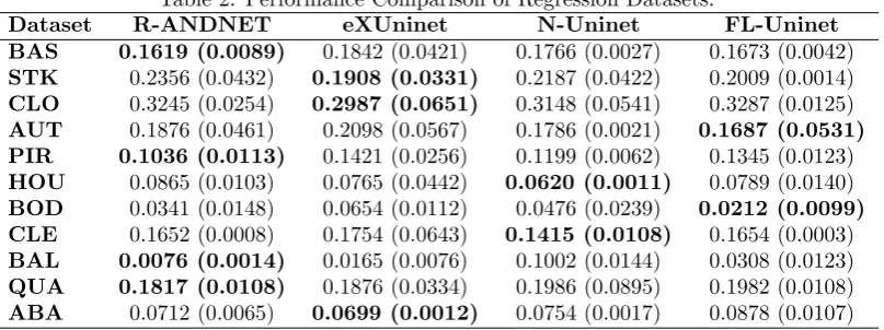
Table 2: Performance Comparison of Regression Datasets.
At first, we verified that the performance of the evaluated algorithms approximates similar behavior, where each of the evaluated models stood out more in a specific context. The proposed model was able to stand out when the number of dimensions of the problem was small. The eXUninet model had its most notable performance when there was a balance between the number of features and a quantity of not so high samples. Another essential factor to be highlighted is that the FL-Uninet model had a better performance in performing the regression when the dimensions were higher (above eight features). As the results were close and it is impossible to identify a trend to the naked eye, statistical tests were used to verify if for each regression set of solving the algorithms had the same behavior [17]. As the test conditions were planned to avoid interfering with undesirable values in the results, we will perform a block variance analysis test [48] to answer the following question: Do the evaluated algorithms have the same RMSE to perform the regression of the 11 proposed classes to the test? As we evaluate the accuracy of the algorithms in 11 bases of different characteristics, we must avoid that the variation of the difficulties of the inputs becomes a source of uncertainty for the problem. Therefore all the source of spurious variation must be controlled. To perform the statistical tests, the analysis of variance (ANOVA) [48] on the results of each of the groups (algorithm x block factor) is used in the test. In general, it is verified that the test has 44 (4 algorithms and 11 bases) groups. Through this test, we intend to conclude if the performance of the algorithms proposed in this paper presents an average performance equal to the other models that are the reference in the literature.
In order to aid in statistical evaluations, we will define as our null hypothesis (H0) that there is no difference
in performance of the algorithms when comparing the RMSE of each of the test blocks in the databases. The alternative hypothesis (H1) is that the algorithms present different RMSE when acting in the linear regression in
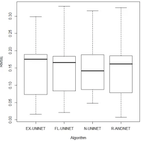
the test bases. The confidence interval adopted for the evaluation of the tests isα= 95In Figure 7 and 8 we can see the plot of the relationship between the evaluated algorithms and the RMSE of the linear regression test.
Figure 7: Plot RMSE x Algorithm.
After the information collected, we created graphs with the information obtained to verify the behavior of the models. In the graphical verification of the data we can verify that the models maintain similar behavior in relation to the RMSE, however to resolve any doubts about the issues of accepting or rejecting the null hypothesis, we performed a test of analysis of variances with the data, obtaining as a response that we must accept the null hypothesis (H0), worth noting that the p-value found was very high: 0.9981. Therefore, we can conclude based
Figure 8: Plot RMSE x Problem.
To confirm the result of the analysis of the variances, three tests were used to validate the normality respec-tively, homoscedasticity and independence of the data collected. To confirm the conditions of normality of the data, we used the Shapiro-Wilk test [48] that resulted in the confirmation of the characters found analyzed. In the homoscedasticity test, which verifies the equality of variances of the residues, the acceptance of the null hypothesis for the Fligner-Killeen test [48] was verified, which informs us that the variances of the residues involved in the analysis are the same. Finally, the Durbin-Watson test [48] confirmed that the null hypothesis of the test could not be rejected, so the data collected have independence.
Figure 9 shows the graphical results of the validation tests of the ANOVA premises.
In order to present in a more detailed way the behavior of the proposed model in comparison to the other models of fuzzy neural networks submitted to the test, we performed the post-hoc test of multiple comparisons of Tukey [48]. The result of this test is shown in Table III.
Table 3: Multiple Comparisons of Means: Tukey Test
Algorithm diff lwr upr. Pr adj FL-UNINET-EX-UNINET -0.003109 -0.086463 0.080245 0.999634 N-UNINET-EX-UNINET 0.001545 -0.081809 0.084900 0.999955 R-ANDNET-EX-UNINET -0.003400 -0.086754 0.079547 0.999522 N-UNINET-FL-UNINET 0.004654 -0.078700 0.088245 0.998779 R-ANDNET-FL-UNINET -0.002909 -0.086463 0.080245 0.999999 R-ANDNET-N-UNINET -0.004945 -0.088302 0.078409 0.998530
Since no rejections of H0 occurred with any of the premise verification tests, we can conclude, with a 95%
confidence interval, that we must accept our null hypothesis for the statistical tests used.
4.2.2 Regularized or pruned methods for regression problems
Figure 9: ANOVA test check.
network can maintain the capacity to perform linear regression and how it behaves in the face of the pruning of neurons through the bolasso. Table IV and Table V present the result of tests.
Table 4: Performance Comparison of Regression Datasets for Regularized Pruning Methods. Dataset R-ANDNET EFOP-ELM OSF-ELM R-ELAFIS BAS 0.1817 (0.0111) 0.1908 (0.0165) 0.2021 (0.0448) 0.2062 (0.0414) STK 0.2816 (0.0546) 0.1799 (0.0423) 0.1987 (0.0074) 0.2941 (0.0364) CLO 0.8642 (0.0642) 0.7654 (0.0115) 0.6668 (0.0712) 0.7681 (0.1008) AUT 0.2071 (0,0876) 0.1815 (0.0532) 0.1987 (0.0101) 0.2245 (0.0436) PIR 0.1276 (0.0008) 0.1343 (0.0876) 0.1619 (0.0421) 0.1513 (0.0778) HOU 0.2019 (0.0876) 0.1876 (0.0477) 0.1987 (0.0722) 0.1543 (0.0765) BOD 0.0259 (0.0123) 0.0324 (0.0176) 0.3531 (0.0044) 0.2780 (0.0654) CLE 0.2034 (0.0076) 0.1124 (0.0163) 0.2173 (0.0345) 0.1876 (0.0089) BAL 0.0156 (0.0053) 0.0311 (0.0048) 0.0221 (0.0017) 0.0421 (0.0654) QUA 0.1973 (0.0301) 0.2134 (0.0412) 0.2396 (0.0972) 0.3498 (0.0498) ABA 0.0567 (0.0126) 0.0341 (0.0103) 0.0442 (0.0112) 0.0245 (0.0341)
Table 5: Final Network Neurons (ls)
Dataset R-ANDNET EFOP-ELM OSF-ELM R-ELAFIS BAS 12.650 (0.756) 22.650 (13.165) 16.761 (6.543) 42.677 (23.158) STK 48.965 (13.985) 67.821 (14.875) 89.087 (9.812) 64.997 (14.833) CLO 67.834 (18.998) 64.560 (9.764) 71.714 (8.701) 89.221 (19.723) AUT 56.412 (12.008) 0.1815 (0.0532) 0.1987 (0.0101) 0.2245 (0.0436) PIR 101.965 (5.983) 106.331 (12.316) 118.650 (14.876) 136.347 (31.331) HOU 78.943 (7.698) 79.516 (9.142) 79.017 (8.765) 81.424 (6.165) BOD 69.113 (15.657) 71.912 (0.987) 70.761 (15.321) 91.817 (0.441) CLE 55.437 (16.842) 62.980 (7.678) 56.111 (8.742) 77.180 (12.016) BAL 5.098 (0.007) 8.000 (0.000) 7.876 (0.987) 7.0870 (0.007) QUA 12.761 (2.098) 10.762 (0.661) 15.531 (4.841) 14.678 (0.890) ABA 32.365 (8.431) 54.812 (12.012) 49.067 (12.150) 44.832 (12.043)
methods analyzed. However, when comparing the number of neurons used. It can be seen that the model proposed in the paper worked on average with an architecture to perform the linear regression of the database.
4.2.3 Fuzzy Rules and interpretation of the results obtained by the model
In order to identify the interpretability of the results. A test with synthetic data was proposed so that the predic-tive capacity of the model is demonstrated graphically and through fuzzy rules. The following code was generated in Matlab to perform the creation of a synthetic. Random and independent base. Seeking to define the better visibility of the facts.
X=[(100:200)’+randn(101.1) (300:400)’+randn(101.1) ones(101.1)]; P1=2; P2=1; P3=100;
Y=P1*X(:.1)+P2*X(:.2)+P3; Y=Y+randn(101.1);
For the test to be performed. considerK = 2 for Gaussian Membership Function. b = 16 andγ = 0.9. In figure 10 presents the Gaussian Membership Functions create in this tests.
Figure 10: Gaussian Membership Function.
The model generated four fuzzy rules in the first layer. This type of approach allows saying that in a group of two characteristics on a Cartesian axis (x1 andx2). Equally spaced membership functions can denote literal
values as small and large. In figure 11 below, consider the abscissa axis asx1 and the ordinate axis as x2. In
figure 12 we can see how the membership functions can help in the division of the data into space.
Figure 11: Hypothetical data used in the regression
In Figure 12 we can see how the membership functions can delimit more representative spaces for the problem. In this presented context, each one of the Gaussian membership functions was given names ofsmall and large. Note that when the ordinate axis has asmall membership function, and the abscissa axis has alarge membership function, there is no data representative of the model.
The same happens when in thex1axis thelarge membership function is represented, and thesmall
Figure 12: Presentation of the hypothetical data used in the regression problem and the Gaussian mem-bership functions.
from the structure of the model. Allowing it to have more representative answers to solve the problem. In this example model we have four fuzzy neurons represented by the following combinations:
1. First Fuzzy Neuron: x1small andx2 small
2. Second Fuzzy Neuron: x1 small andx2 large
3. Third Fuzzy Neuron: x1 large andx2 small
4. Fourth Fuzzy Neuron: x1 large andx2 large
The method of regularization will eliminate two fuzzy neurons that do not present data in this problem (second and third), will have two neurons that are more representative of the problem, thus allowing to build fuzzy rules (5) of each of the andneuron.
For the four fuzzy neurons resulting from this experiment, we can conclude the following fuzzy rules:
Rule1: Ifxi1 issmallwith certainty 0.7139
andxi2 issmallwith certainty 0.5207
Theny1is 0.6180
Rule2: Ifxi1 issmallwith certainty 0.2607
andxi2 islargewith certainty 0.8759
Theny2is 0.1968
Rule3: Ifxi1 islargewith certainty 0.6297
andxi2 issmallwith certainty 0.4699
Theny3is−1.0633
Rule4: Ifxi2 islargewith certainty 0.4196
andxi2 islargewith certainty 0.5207
Theny4is 0.2851 (14)
In this context, we can demonstrate several relationships, for example, suppose that x1 is the value of an
invoice andx2 represents taxes. The response variable may be the value of a person’s debts. When the value of
invoices and taxes are low the value of the person’s debts will be low. Likewise, when invoice and tax amounts are high, the person’s spending forecast will be high. This type of rule assists in the creation of expert systems, to assist in the prediction of factors that may or may not impact the linear regression of a studied context.
5
Conclusion
This paper has introduced a new learning algorithm for fuzzy neural networks based on ideas from Extreme Learning Machine and regularization theory for regression problems. Random parameters are defined for the second layer neurons, and the bootstrap lasso algorithm is used to generate sparse models. The experiments performed and the results suggest the network as a promising alternative to build accurate and transparent models. The statistical tests confirmed that the fuzzy neural network could behave as a universal approximation, performing linear regressions equivalent to models widely used in the literature and maintains a leaner architecture with regularization techniques, allowing the hidden layer of the model to use the lowest mean number of neurons to perform their activities. As the cross-validation method becomes a little expensive in the choice of network parameters, new optimization techniques for the choice of input parameters of the model may be the subject of future research. Future work shall address methods to improve the network interpretability and evaluation on multi-class classification problems. In future work, the model can be adapted to incorporate convolutions, deep learning concepts and think of new techniques of data fuzzification [61] and [45] for example, so that the model does not have its performance on creating membership functions proportional to the number of dimensions and/or samples.
Acknowledgements
The thanks of this work are for CEFET-MG and UNA Betim.
References
[1] Plamen Angelov. Evolving Takagi-Sugeno Fuzzy Systems from Streaming Data (eTS+), chapter 2, pages 21–50. Wiley-Blackwell, 2010.
[2] Plamen Angelov and Ronald Yager. A new type of simplified fuzzy rule-based system.International Journal of General Systems, 41(2):163–185, 2012.
[3] Francis R Bach. Bolasso: model consistent lasso estimation through the bootstrap. InProceedings of the 25th international conference on Machine learning, pages 33–40. ACM, 2008.
[4] Rosangela Ballini and Fernando Gomide. Learning in recurrent, hybrid neurofuzzy networks. In Fuzzy Systems, 2002. FUZZ-IEEE’02. Proceedings of the 2002 IEEE International Conference on, volume 1, pages 785–790. IEEE, 2002.
[6] Catherine Blake. Uci repository of machine learning databases. http://www. ics. uci. edu/˜ mlearn/MLRepository. html, 1998.
[7] F. Bordignon and F. Gomide. Extreme learning for evolving hybrid neural networks. In 2012 Brazilian Symposium on Neural Networks, pages 196–201, Oct 2012.
[8] Fernando Bordignon and Fernando Gomide. Uninorm based evolving neural networks and approximation capabilities. Neurocomputing, 127:13–20, 2014.
[9] A de P Braga, APLF Carvalho, and Teresa Bernarda Ludermir.Redes neurais artificiais: teoria e aplica¸c˜oes. Livros T´ecnicos e Cient´ıficos Rio de Janeiro, 2000.
[10] Walmir M Caminhas, Hermano Tavares, Fernando AC Gomide, and Witold Pedrycz. Fuzzy set based neural networks: Structure, learning and application. JACIII, 3(3):151–157, 1999.
[11] P. V. de Campos Souza and P. F. A. de Oliveira. Regularized fuzzy neural networks based on nullneurons for problems of classification of patterns. In 2018 IEEE Symposium on Computer Applications Industrial Electronics (ISCAIE), pages 25–30, April 2018.
[12] P. V. de Campos Souza, G. R. L. Silva, and L. C. B. Torres. Uninorm based regularized fuzzy neural networks. In2018 IEEE Conference on Evolving and Adaptive Intelligent Systems (EAIS), pages 1–8, May 2018. [13] Paulo Vitor de Campos Souza. Pruning fuzzy neural networks based on unineuron for problems of
classifi-cation of patterns. Journal of Intelligent and Fuzzy Systems, 35:2597–2605, 2018.
[14] Paulo Vitor de Campos Souza and Luiz Carlos Bambirra Torres. Regularized fuzzy neural network based on or neuron for time series forecasting. In Guilherme A. Barreto and Ricardo Coelho, editors,Fuzzy Information Processing, pages 13–23, Cham, 2018. Springer International Publishing.
[15] J. C. Dunn. A fuzzy relative of the isodata process and its use in detecting compact well-separated clusters.
Journal of Cybernetics, 3(3):32–57, 1973.
[16] Bradley Efron, Trevor Hastie, Iain Johnstone, Robert Tibshirani, et al. Least angle regression. The Annals of statistics, 32(2):407–499, 2004.
[17] Jerome Friedman, Trevor Hastie, and Robert Tibshirani. The elements of statistical learning, volume 1. Springer series in statistics New York, NY, USA:, 2001.
[18] Federico Girosi, Michael Jones, and Tomaso Poggio. Regularization theory and neural networks architectures.
Neural computation, 7(2):219–269, 1995.
[19] Adam F Gobi and Witold Pedrycz. Logic minimization as an efficient means of fuzzy structure discovery.
IEEE Transactions on Fuzzy Systems, 16(3):553–566, 2008.
[20] Gene Golub and William Kahan. Calculating the singular values and pseudo-inverse of a matrix. Journal of the Society for Industrial and Applied Mathematics, Series B: Numerical Analysis, 2(2):205–224, 1965. [21] Serge Guillaume. Designing fuzzy inference systems from data: An interpretability-oriented review. IEEE
transactions on fuzzy systems, 9(3):426–443, 2001.
[22] Trevor Hastie, Robert Tibshirani, and Jerome Friedman. Unsupervised learning. InThe elements of statistical learning, pages 485–585. Springer, 2009.
[23] Trevor Hastie, Robert Tibshirani, and Jerome H. Friedman.The elements of statistical learning: data mining, inference, and prediction, 2nd Edition. Springer series in statistics. Springer, 2009.
[24] S. Haykin. Redes Neurais: Princ´ıpios e Pr´atica. Artmed, 2007.
[25] Simon Haykin. Neural networks: a comprehensive foundation. Prentice Hall PTR, 1994.
[26] Michel Hell, Pyramo Costa, and Fernando Gomide. Participatory learning in power transformers thermal modeling. IEEE Transactions on Power Delivery, 23(4):2058–2067, 2008.
[27] Michel Hell, Fernando Gomide, Rosangela Ballini, and Pyramo Costa. Uninetworks in time series forecasting. InFuzzy Information Processing Society, 2009. NAFIPS 2009. Annual Meeting of the North American, pages 1–6. IEEE, 2009.
[28] Michel Bortolini Hell et al. Abordagem neurofuzzy para modelagem de sistemas dinamicos n˜ao lineares. 2008.
[29] F. Herrera, M. Lozano, and J.L. Verdegay. Tackling real-coded genetic algorithms: Operators and tools for behavioural analysis. Artificial Intelligence Review, 12(4):265–319, Aug 1998.
[30] Arthur E Hoerl and Robert W Kennard. Ridge regression: Biased estimation for nonorthogonal problems.
[31] G. Huang, H. Zhou, X. Ding, and R. Zhang. Extreme learning machine for regression and multiclass classi-fication. IEEE Transactions on Systems, Man, and Cybernetics, Part B (Cybernetics), 42(2):513–529, April 2012.
[32] Guang-Bin Huang and Lei Chen. Convex incremental extreme learning machine. Neurocomputing, 70(16):3056 – 3062, 2007. Neural Network Applications in Electrical Engineering Selected papers from the 3rd International Work-Conference on Artificial Neural Networks (IWANN 2005).
[33] Guang-Bin Huang, Lei Chen, and Chee-Kheong Siew. Universal approximation using incremental construc-tive feedforward networks with random hidden nodes.Trans. Neur. Netw., 17(4):879–892, July 2006. [34] Guang-Bin Huang, Lei Chen, Chee Kheong Siew, et al. Universal approximation using incremental
con-structive feedforward networks with random hidden nodes. IEEE Trans. Neural Networks, 17(4):879–892, 2006.
[35] Guang-Bin Huang, Qin-Yu Zhu, and Chee-Kheong Siew. Extreme learning machine: a new learning scheme of feedforward neural networks. In Neural Networks, 2004. Proceedings. 2004 IEEE International Joint Conference on, volume 2, pages 985–990. IEEE, 2004.
[36] Guang-Bin Huang, Qin-Yu Zhu, and Chee-Kheong Siew. Extreme learning machine: theory and applications.
Neurocomputing, 70(1-3):489–501, 2006.
[37] J-SR Jang. Anfis: adaptive-network-based fuzzy inference system.IEEE transactions on systems, man, and cybernetics, 23(3):665–685, 1993.
[38] J. Kim and N. Kasabov. Hyfis: adaptive neuro-fuzzy inference systems and their application to nonlinear dynamical systems. Neural Networks, 12(9):1301 – 1319, 1999.
[39] Ron Kohavi. A study of cross-validation and bootstrap for accuracy estimation and model selection. In
Proceedings of the 14th International Joint Conference on Artificial Intelligence - Volume 2, IJCAI’95, pages 1137–1143, San Francisco, CA, USA, 1995. Morgan Kaufmann Publishers Inc.
[40] Shihabudheen KV and G.N. Pillai. Regularized extreme learning adaptive neuro-fuzzy algorithm for regres-sion and classification. Know.-Based Syst., 127(C):100–113, July 2017.
[41] Andre Lemos, Walmir Caminhas, and Fernando Gomide. New uninorm-based neuron model and fuzzy neural networks. InFuzzy Information Processing Society (NAFIPS), 2010 Annual Meeting of the North American, pages 1–6. IEEE, 2010.
[42] Andre Paim Lemos, Walmir Caminhas, and Fernando Gomide. A fast learning algorithm for uninorm-based fuzzy neural networks. In Fuzzy Information Processing Society (NAFIPS), 2012 Annual Meeting of the North American, pages 1–6. IEEE, 2012.
[43] Xiaofeng Liang and Witold Pedrycz. Logic-based fuzzy networks: a study in system modeling with triangular norms and uninorms. Fuzzy sets and systems, 160(24):3475–3502, 2009.
[44] E. Lima, F. Gomide, and R. Ballini. Participatory evolving fuzzy modeling. In2006 International Symposium on Evolving Fuzzy Systems, pages 36–41, Sept 2006.
[45] Jingjing Ma, Xiangming Jiang, and Maoguo Gong. Two-phase clustering algorithm with density exploring distance measure. CAAI Transactions on Intelligence Technology, 3(1):59–64, 2018.
[46] Jos´e M Mart´ıNez-Mart´ıNez, Pablo Escandell-Montero, Emilio Soria-Olivas, Jos´e D Mart´ıN-Guerrero, Rafael Magdalena-Benedito, and Juan G´oMez-Sanchis. Regularized extreme learning machine for regression prob-lems. Neurocomputing, 74(17):3716–3721, 2011.
[47] M Mike. Statistical datasets. Dept. Statist., Univ. Carnegie Mellon, Pittsburgh, PA, 1989.
[48] D.C. Montgomery. Design and Analysis of Experiments. Student solutions manual. John Wiley & Sons, 2008.
[49] Wim De Mulder, Steven Bethard, and Marie-Francine Moens. A survey on the application of recurrent neural networks to statistical language modeling. Computer Speech Language, 30(1):61 – 98, 2015.
[50] Witold Pedrycz. Fuzzy neural networks and neurocomputations. Fuzzy Sets and Systems, 56(1):1–28, 1993. [51] Witold Pedrycz. Heterogeneous fuzzy logic networks: fundamentals and development studies. IEEE
Trans-actions on Neural Networks, 15(6):1466–1481, 2004.
[52] Witold Pedrycz. Logic-based fuzzy neurocomputing with unineurons.IEEE Transactions on Fuzzy Systems, 14(6):860–873, 2006.
[54] Witold Pedrycz and Fernando Gomide. Fuzzy systems engineering: toward human-centric computing. John Wiley & Sons, 2007.
[55] Alok Porwal, E. J. M. Carranza, and M. Hale. A hybrid neuro-fuzzy model for mineral potential mapping.
Mathematical Geology, 36(7):803–826, Oct 2004.
[56] Federico Montesino Pouzols and Amaury Lendasse. Evolving fuzzy optimally pruned extreme learning ma-chine for regression problems. Evolving Systems, 1(1):43–58, 2010.
[57] Christian Robert. Machine learning, a probabilistic perspective, 2014.
[58] H. Rong, G. Huang, N. Sundararajan, and P. Saratchandran. Online sequential fuzzy extreme learning machine for function approximation and classification problems. IEEE Transactions on Systems, Man, and Cybernetics, Part B (Cybernetics), 39(4):1067–1072, Aug 2009.
[59] R. Rosa, F. Gomide, and R. Ballini. Evolving hybrid neural fuzzy network for system modeling and time series forecasting. In2013 12th International Conference on Machine Learning and Applications, volume 2, pages 378–383, Dec 2013.
[60] Paulo Vitor C Souza. Regularized fuzzy neural networks for pattern classification problems. International Journal of Applied Engineering Research, 13(5):2985–2991, 2018.
[61] Jun Wu and Xin Xu. Decentralised grid scheduling approach based on multi-agent reinforcement learning and gossip mechanism. CAAI Transactions on Intelligence Technology, 3(1):8–17, 2018.
![Figure 2: Example of networks feedforward and networks recurrent. [49]](https://thumb-us.123doks.com/thumbv2/123dok_us/8807311.1775275/4.595.199.426.243.354/figure-example-networks-feedforward-networks-recurrent.webp)