www.biogeosciences.net/6/1341/2009/
© Author(s) 2009. This work is distributed under the Creative Commons Attribution 3.0 License.
Biogeosciences
Improving land surface models with FLUXNET data
M. Williams1, A. D. Richardson2, M. Reichstein3, P. C. Stoy4, P. Peylin5, H. Verbeeck6, N. Carvalhais7, M. Jung3, D. Y. Hollinger8, J. Kattge3, R. Leuning9, Y. Luo10, E. Tomelleri3, C. M. Trudinger11, and Y. -P. Wang11
1School of GeoSciences and NERC Centre for Terrestrial Carbon Dynamics, University of Edinburgh, Edinburgh, UK 2University of New Hampshire, Complex Systems Research Center, Durham, USA
3Max Planck Institute for Biogeochemistry, Jena, Germany 4School of GeoSciences, University of Edinburgh, Edinburgh, UK
5Laboratoire des sciences du climat et de l’environnement (LSCE), Gif Sur Yvette, France 6Laboratory of Plant Ecology, Ghent University, Belgium
7Faculdade de Ciˆencias e Tecnologia, Universidade Nova de Lisboa, Caparica, Portugal 8Northern Research Station, USDA Forest Service, Durham, NH, USA
9CSIRO Marine and Atmospheric Research Canberra ACT 2601, Australia
10Department of Botany and Microbiology, University of Oklahoma, Norman, OK 73019, USA 11CSIRO Marine and Atmospheric Research, Centre for Australian Weather and Climate Research,
Aspendale, Victoria, Australia
Received: 15 January 2009 – Published in Biogeosciences Discuss.: 5 March 2009 Revised: 19 June 2009 – Accepted: 2 July 2009 – Published: 30 July 2009
Abstract. There is a growing consensus that land surface models (LSMs) that simulate terrestrial biosphere exchanges of matter and energy must be better constrained with data to quantify and address their uncertainties. FLUXNET, an international network of sites that measure the land surface exchanges of carbon, water and energy using the eddy covari-ance technique, is a prime source of data for model improve-ment. Here we outline a multi-stage process for “fusing” (i.e. linking) LSMs with FLUXNET data to generate bet-ter models with quantifiable uncertainty. First, we describe FLUXNET data availability, and its random and systematic biases. We then introduce methods for assessing LSM model runs against FLUXNET observations in temporal and spatial domains. These assessments are a prelude to more formal model-data fusion (MDF). MDF links model to data, based on error weightings. In theory, MDF produces optimal analy-ses of the modelled system, but there are practical problems. We first discuss how to set model errors and initial condi-tions. In both cases incorrect assumptions will affect the outcome of the MDF. We then review the problem of equi-finality, whereby multiple combinations of parameters can produce similar model output. Fusing multiple independent
Correspondence to: M. Williams ([email protected])
25 904
905 906 907
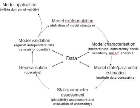
Figure 1 The multi-stage process for model-data fusion: a conceptual diagram showing the main steps (and the iterative nature of these steps) involved in a comprehensive data-model fusion.
Fig. 1. The multi-stage process for model-data fusion: a conceptual
diagram showing the main steps (and the iterative nature of these steps) involved in a comprehensive data-model fusion.
1 Introduction
Land surface models are important tools for understanding and predicting mass and energy exchange between the ter-restrial biosphere and atmosphere. A land surface model (LSM) is a typical and critical component of larger domain models, which are aimed at global integration, for example global carbon cycle models and prognostic global climate models. These integrated models are key tools for predict-ing the likely future states of the Earth system under anthro-pogenic forcing (IPCC, 2007), and for assessing feedbacks with, and impacts on, the biosphere (MEA, 2005). Land sur-face models represent the key processes regulating energy and matter exchange – photosynthesis, respiration, evapo-transpiration (Bonan, 1995; Foley et al., 1996; Williams et al., 1996; Sellers et al., 1997), and their coupling. These processes are sensitive to environmental drivers on a range of timescales, for example, responding to diurnal changes in insolation, and seasonal shifts in temperature and precip-itation. Land surface processes influence the climate sys-tem, through their control of energy balance and greenhouse gas exchanges. Forecasts of global terrestrial C dynamics that rely on LSMs show significant variability over decadal timescales (Friedlingstein et al., 2006), especially when cou-pled to climate, indicating that major uncertainties remain in the representation of critical ecosystem processes and cli-mate feedbacks within global models.
In recent years the widespread use of the eddy covari-ance (EC) methodology has led to a large increase in data on terrestrial land surface exchanges (Baldocchi et al., 2001). FLUXNET is an international network of EC sites with data processed according to standardized protocols (Papale et al., 2006). The EC time-series data from FLUXNET provide rich insights into exchanges of water, energy and CO2 across a
range of biomes and timescales. While LSM forward runs are commonly compared with EC data, there is a grow-ing consensus that models must be better constrained with such data to address process uncertainty (Bonan, 2008). A stronger link between models and observations is needed to identify poorly represented or missing processes, and to pro-vide confidence intervals on model parameter estimates and forecasts.
New methods are becoming available to assist data anal-ysis and generate links to models, based on the concept of model-data fusion, MDF (Raupach et al., 2005). MDF en-compasses a range of procedures for combining a set or sets of observations and a model, while quantitatively incorporat-ing the uncertainties of both. MDF is used to estimate model states and/or parameters, and their respective uncertainties.
The objective of this paper is to provide guidance to the LSM community on how to make better use of eddy covari-ance data, particularly via MDF. We first outline the philo-sophical principles behind model-data fusion for model im-provement. We then discuss the structure of typical land sur-face models and how they are parameterised. Next we de-tail FLUXNET data availability and quality, specifically in the context of land surface models. We discuss approaches for model and data evaluation, focussing on new techniques using time series and spatial analyses. Finally we discuss formal model-data fusion and highlight the need for multiple constraints in model evaluation and improvement, and effec-tive assessment of model and data errors. We conclude with a set of challenges for the LSM and MDF communities.
2 The philosophy of model-data fusion for model improvement
[image:2.595.51.286.61.243.2]Table 1. Land surface model components and details, after Liu and Gupta (2007).
Model component Examples for typical LSMs
System boundary Lower atmosphere, deep soil/geological parent material
Forcing inputs Air temperature, short and long-wave radiation, precipitation, wind speed, vapour pressure deficit,
atmospheric CO2concentration
Initial states Biogeochemical pools, vegetation and soil temperature and water content
Parameters Rate constants for chemical processes, physical constants, biological parameters
Model structure Process definitions and connectivity
Model states Biogeochemical pools, vegetation and soil temperature and water content
Outputs Biogeochemical fluxes, dynamics of model states
observations. If so, model deficiencies can be clearly located. If model parameter estimation is the goal, then model param-eters are adjusted so that the model state(s) come into closer agreement with the observations. Following the optimization of model parameters (defined here loosely to potentially in-clude both parameters sensu stricto and state variables), it is vitally important that further analyses be conducted by the modeller to: (1) quantify uncertainties in optimized param-eters (and thus identify those paramparam-eters, and related pro-cesses, that are poorly constrained by the data); (2) evaluate the plausibility and temporal stability of optimized parame-ter values (reality check); (3) understand when and why the model is failing (“detective work”, which may involve addi-tional validation against independent data sets); and (4) iden-tify opportunities for model improvement (re-formulation of structure and process representation). When treated in this manner, MDF has relevance to both basic and applied scien-tific questions. Thus, not only do identified deficiencies lead to model reformulation (followed by further data-model fu-sion, possibly with new data sets being brought to bear), but the model can also be applied to answer new science ques-tions. Successful application of the model is, however, con-tingent on the modeller’s understanding (which comes from the posterior analyses) of the domain (in terms of space, time, and prognostic variables), where the model can be applied with precision and confidence.
3 Land surface models
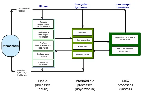
All models consist of seven general components; the system boundary, forcing inputs, initial states, parameters, model structure, model states, and outputs (Liu and Gupta, 2007). The details of these components for typical LSMs are given in Table 1. These are physical, chemical and biological pro-cesses, related to fluxes of energy, water and carbon, that are sensitive to changes in environmental forcing on multiple time scales (Fig. 2). Models differ as to whether they also represent processes operating on longer time scales. Some models link CO2fluxes to plant traits such as allocation,
lit-ter production, phenology, vegetation dynamics and compe-tition, while others rely on prescribed inputs of vegetation
Canopy conductance photosynthesis,
leaf respiration
Vegetation dynamics & disturbance Land-use and land-cover change Autotrophic and
Heterotrophic respiration
Phenology Turnover Solution of SEB;
canopy and ground temperatures
and fluxes
Soil heat and moisture Surface water
balance
Atmosphere
Fluxes Ecosystem dynamics
Landscape dynamics
Canopy conductance, photosynthesis
Vegetation dynamics & disturbance
Land use and land cover change Allocation
Phenology Litter production
Nutrient cycles Surface
temperatures and heat fluxes
Soil heat and moisture Surface water
balance Autotrophic & heterotrophic respiration Atmospheric forcing
Radiation, H2O, CO2&
heat fluxes
Rapid processes
(hours)
Intermediate processes (days-weeks)
Slow processes
(years+)
908 909 910 911
Figure 2. Schematic of a typical land surface model. LSMs include a range of processes operating on different scales. LSMs can be driven by atmospheric observations or
analyses, or directly coupled to atmospheric models. All LSMs tend to represent the hourly processes, but daily and annual processes may not be included.
26
Fig. 2. Schematic of a typical land surface model. LSMs include
a range of processes operating on different scales. LSMs can be driven by atmospheric observations or analyses, or directly coupled to atmospheric models. All LSMs tend to represent the hourly pro-cesses, but daily and annual processes may not be included.
structure to drive flux predictions. Here, we focus largely on models that couple fluxes to the dynamics of structural C pools, as only these models are capable of prediction over decadal timescales.
[image:3.595.309.547.221.378.2]27 912
(A)
(B)
-20 -10 0 10 20 30
Tair_f [°C] 0 1000 2000 3000 4000 p rec ip_f [ m m da y -1] AT AT AT AT AUAU AU AU AU AU AU BE BE BE BE BE BE BE BEBE BE BE BE BE BE BE BE AU AU AU BRBR BR BR BR BR BR BR BR BR CA CA CA CACA CACA CA CA CA CACA CA CA CA CA CA CACA CA CACACACA CA CACA CA CA CA CA CA CA CA CA CA CA CACA CA CACA CA
CACACA
CA CA CACA CACA CA CA CA CA CA CA CA CA CA CA CA CA CA CA CA
CACACA
CA CA CA CA CA CA CA CA CA CH CH CH CH CH CN CN CN CN DE DE DE DE DE DE DEDE DE DE DE DE DEDE DE DE DE DE
DEDEDE DEDE DE DE DE DEDE DE DE DE DE DE DE DK DK DK DKDK DKDK DK DK DK DK DK DK ES
ESESES S ES ESES ES ESES ES FI FI FI FI FI FIFIFI FI FIFI FI FIFI FI FI FR FR FR FR FR FR FR FRFR FR FR FR FR FR FR FRFR FR FR FR FR FR FR FR FR FRFR FR FR
HUHUIE IE IE IE IE IT IT IT IT IT IT BR BR US US BW GF GF GF ID ID VU CN S CN CN FR IT IT E US FR IL IT IT IT IL US US IT US IT IT IT IT IT IT IT IT IT ITIT IT IT IT ITIT JP US US US US IT IT IT IT IT IT ITIT IT J JPJP JP JP JP KR NL NL NLNL NL NLNL NL NL NL NL NL NL NL NL NLNL PL TPT PT PT PT PT PT PT RU RURU SE SE SE UK UK UK UK UK UK UK UK
USUSUS
U USUS US US US US US USUS US US US US US US US
USUSUS USUSUSUS US IT IT P IT IT IT P PT PT US S US KR
USUSUS US US US US US US USUS US US US US US US US US US US USUS US US US US US US US US US US US US US US US USUS US US US US US US US US US US US US US USUS US US U US US US US US US US US US US US US US US US US USUS US US US US US US US US S S US US U US US U US US US US US USUS US US USUS US
US USUSUS
USUS USUS US
US USUSUS
US US US US US US US USUSUS
US US Us Us VU ZA ZA Ann ual prec ipit at io n [ m m] 913 914 915 916 917 918 919 17.5 20.0 22.5 25.0 27.5 30.0 32.5 35.0 16.0 36.0
Mean annual temperature [°C]
Figure 3 Distribution of sites that are present in the current La-THuile 2007 FLUXNET database. (a) Geographical distribution, (b) in climate (annual temperature and precipitation ) space. In b) colours code annual potential shortwave radiation flux density [MJ m-2 day-1] according to the legend. Letters are country
codes.
Fig. 3. Distribution of sites that are present in the current La-THuile
2007 FLUXNET database. (a) Geographical distribution, (b) in cli-mate (annual temperature and precipitation) space. In (b) colours
code annual potential shortwave radiation flux density [MJ m−2
day−1] according to the legend. Letters are country codes.
Differences among LSMs in structure and parameterisa-tion mean that they have different response funcparameterisa-tions relat-ing rates of carbon and water fluxes to global change fac-tors (e.g., CO2concentration, temperature, and precipitation
or soil moisture content). Subtle changes to response func-tions and parameterizafunc-tions can yield divergent modelled re-sponses of ecosystems to environmental change, as has been demonstrated by parameter sensitivity studies (e.g. Zaehle et al., 2005; White et al., 2000) and model intercomparisons (e.g. Friedlingstein et al., 2006; Jung et al., 2007). Differ-ences in the way processes interact in the model are also likely candidates for divergent model behaviour, but even harder to detect than differences in process representation (Rastetter, 2003). Rigorous comparison with data provides the basis for better constraining model structure and for gen-erating more defensible parameter estimates with realistic uncertainty estimates.
4 Data availability, limitations and challenges 4.1 Overall overview
Continuous measurements of surface-atmosphere CO2
ex-change using the eddy covariance technique started in 1990s (Verma, 1990; Baldocchi, 2003). Consequently, many EC observation sites have been established, leading to the de-velopment of regional networks, such as AmeriFlux and Eu-roflux, and then the global network FLUXNET, a “network of regional networks” (Baldocchi et al., 2001). The need for harmonized data processing has been recognized in the different networks, and respective processing schemes docu-mented in the literature (Foken and Wichura, 1996; Aubinet et al., 2000; Falge et al., 2001; Reichstein et al., 2005; Papale et al., 2006; Moffat et al., 2007). A first cross-network stan-dardized dataset was established in 2000 (Marconi dataset) and contained data from 38 sites from North America and Europe. In 2007 the first global standardized data set (“La-Thuile FLUXNET dataset”, cf. http://www.fluxdata.org) was established.
4.2 Current distribution and representativeness of flux sites
[image:4.595.51.282.71.355.2]Table 2. Distribution of sites in the current FLUXNET La-Thuile data set with respect to climate and vegetation classes. Climate is
defined according to aggregated Kppen-Geiger classification, cf. www.fluxdata.org. Vegetation classes (top line) are from IGBP definitions: Croplands, closed shrublands, deciduous broadleaf forest, evergreen broadleaf forest, evergreen needleleaf forest, grassland, mixed forest, open shrublands, savanna, wetlands, woody savanna.
Number of Sites available CRO CSH DBF EBF ENF GRA MF OSH SAV WET WSA Total
Tropical 1 0 0 10 0 1 0 1 1 0 2 16
Dry: 0 0 0 1 1 3 0 1 1 0 3 10
Subtropical/mediterranean: 5 3 11 5 17 11 2 3 2 0 4 63
Temperate 17 0 8 2 12 18 4 0 0 4 0 65
Temperate continental 7 1 9 1 17 7 8 3 0 0 0 53
Boreal 0 0 2 0 22 4 2 4 0 4 0 38
Arctic 0 0 2 0 0 1 0 0 0 3 0 6
Total 30 4 32 19 69 45 16 12 4 11 9 251
forest inventories, e.g. US Forest Inventory and Analysis Pro-gram (Gillespie et al., 1999).
4.3 Data characteristics and limitations
The global network of eddy covariance towers not only pro-vides flux observations themselves but also the infrastructure necessary to study ecosystem processes, and relationships between ecosystem processes and environmental forcing, across a range of spatial and temporal scales. The time av-eraging of the measurements (typically either 30 or 60 min) is adequate to resolve both diurnal cycles and fast ecosystem responses to changes in weather. In addition to the measured fluxes (typically CO2 as well as latent and sensible heat)
and enviro-meteorological data, many sites maintain a pro-gramme of comprehensive ecological measurements, includ-ing detailed stand inventories, litterfall collections, soil res-piration and leaf-level photosynthesis, soil and foliar chem-istry, phenology and leaf area index.
However, a careful consideration of the limitations of the data is mandatory to avoid overinterpretation of model-data mismatches in evaluation or assimilation schemes. Flux data are noisy and potentially biased, containing the “true” flux, plus both systematic and random errors and uncertainties (Table 3). There is a growing recognition within the EC com-munity on the need to quantify the random errors inherent in half-hourly flux measurements (Hollinger and Richardson, 2005; Richardson et al., 2006), but also uncertainties in the corrections of systematic errors. Because data uncertainties enter directly into model-data fusion (see below), misspeci-fication of data uncertainties affects parameter estimates and propagates into the model predictions, leading Raupach et al. (2005) to suggest that “data uncertainties are as important as data values themselves”.
Recent research, using data from sites in both North Amer-ica (Richardson et al., 2006) and Europe (Richardson et al., 2008), indicates that the random error scales with the mag-nitude of the flux, thus violating one key assumption (ho-moscedasticity) underlying ordinary least squares
optimiza-100 200 300
0.0 0.2 0.4 0.6 0.8 1.0
Day of year
Fr
a
c
ti
on of
a
bs
obe
d
P
A
R
0.2 0.4 0.6 0.8 1.0 1
920
921 922 923 924 925 926 927
[image:5.595.252.538.128.382.2]928
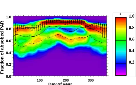
Figure 4 Temporal development of MODIS fPAR-estimates during 2002 at the French Puéchabon FLUXNET
site, an evergreen broadleaf forest (Holm Oak). Diamonds indicate the time series at the tower-pixel, vertical
lines denote between-pixel standard deviation of 3x3 pixels around the tower. Colours code the frequency of
pixels within 100x100 km around the tower having the respective fPAR at the day of the year indicated on the
x-axis. Solid and dashed lines indicate median, lower and upper quartile fPAR over all pixels 100x100km around
the tower. It can be seen that the tower represents the more productive portion of the landscape (assuming
FPAR is a proxy for productivity).
28
Fig. 4. Temporal development of MODIS fPAR-estimates dur-ing 2002 at the French Puchabon FLUXNET site, an evergreen broadleaf forest (Holm Oak). Diamonds indicate the time series at the tower-pixel, vertical lines denote between-pixel standard de-viation of 3×3 pixels around the tower. Colours code the frequency
of pixels within 100×100 km around the tower having the
respec-tive fPAR at the day of the year indicated on the x-axis. Solid and dashed lines indicate median, lower and upper quartile fPAR over
all pixels 100×100 km around the tower. It can be seen that the
tower represents the more productive portion of the landscape (as-suming FPAR is a proxy for productivity).
tion. On the other hand, Lasslop et al. (2008) analysed fur-ther properties of the random error component and found little temporal autocorrelation and cross-correlation of the H2O and CO2 flux errors, implying that the weighted least
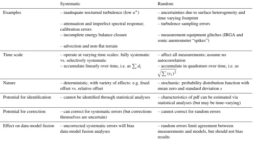
[image:5.595.312.545.239.384.2]Table 3. Characteristics of systematic and random uncertainties in eddy covariance measurements of surface-atmosphere exchanges of CO2,
H2O and energy.
Systematic Random
Examples – inadequate nocturnal turbulence (lowu∗) – uncertainties due to surface heterogeneity and
time varying footprint – attenuation and imperfect spectral response;
calibration errors
– turbulence sampling errors
– incomplete energy balance closure – measurement equipment glitches (IRGA and
sonic anemometer “spikes”) – advection and non-flat terrain
Time scale – operate at varying time scales: fully systematic
vs. selectively systematic
– affect all measurements; assume no autocorrelation
– accumulate linearly over time, i.e. asP
di – accumulate in quadrature over time, i.e. as
q P
(εi)2
Nature – deterministic, with variety of effects: e.g. fixed
offset vs. relative offset
– stochastic: probability distribution function with
mean zero and standard deviations
Potential for identification – cannot be identified through statistical analyses – characteristics of pdf can be estimated via
statistical analyses (but may be time-varying)
Potential for correction – can correct for systematic errors (but corrections
themselves are uncertain)
– cannot correct for random errors
Effect on data-model fusion – uncorrected systematic errors will bias
data-model fusion analyses
– random errors limit agreement between measurements and models, but should not bias results
as independent errors, typically resulting in an uncertainty
<50 g C m−2yr−1 (Richardson et al., 2006; Lasslop et al., 2009). However, the characterization of the statistical prop-erties of flux measurement error remains currently under de-bate and probably varies between sites and environmental conditions (Richardson et al., 2006; Lasslop et al., 2008).
Systematic flux biases are less easily evaluated, but are certainly non-trivial (Goulden et al., 1996; Moncrieff et al., 1996; Baldocchi, 2003). One major source of bias is in-correct measurement of net ecosystem exchange under low-turbulence conditions, especially at night. Attempts to mini-mize this bias use so-calledu∗-filtering (Papale et al., 2006), in which measurements are rejected when made under condi-tions of low turbulence (i.e. below a threshold friction veloc-ity). However, the threshold value foru∗is often uncertain. Preliminary analysis of the La Thuile data set indicated that the uncertainty introduced varies between sites, and can be
>150 gC m−2yr−1in some cases (Reichstein et al., unpub-lished data); hence a careful analysis of this effect is war-ranted.
Energy balance closure at most sites is poor: the sum of sensible, latent and soil heat fluxes is generally∼20% lower than the total available radiative energy, which may indicate systematic errors in measured CO2 fluxes as well (Wilson
et al., 2002). Advection is believed to occur at many sites, particularly those with tall vegetation, and is thought to bias
annual estimates of net sequestration upwards, i.e. more neg-ative NEE (Lee, 1998). While these (and other) system-atic errors are known to affect flux measurements, much less is known about how to adequately quantify and correct for them; typically the time scale at which the correction needs to be applied, and in some cases even the direction of the appropriate correction, is highly uncertain (see discussion in Richardson et al., 2008).
Although attempts are made to make continuous flux mea-surements, in reality there are gaps in the flux record. These gaps most often occur when conditions are unsuitable for making measurements (e.g., periods of rain or low turbu-lence), or as a result of instrument failure. A variety of meth-ods have been proposed and evaluated for filling these gaps and producing continuous time series; the best methods ap-pear to approach the limits imposed by the random flux mea-surement errors described above (e.g., Moffat et al., 2007). In general, MDF will want to use only measured, and not gap-filled, data, because gap-filling involves the use of a model and so can contaminate the MDF. However, in some cases (if, for example, the model time step is different from that of the data, e.g. daily) it may be necessary to resort to using gap-filled data, in which case it is important that the distinction between “measured” and “filled” data be understood.
measurements reflect the net ecosystem exchange (NEE) of CO2, whereas the process-related quantities of interest are
typically the component fluxes, gross photosynthesis (GPP) and ecosystem respiration (RE; also the above- and
below-ground, and autotrophic and heterotrophic, components of ecosystem respiration), which, unlike NEE, represent dis-tinct sets of physiological activity. In a model-data fusion context, the net flux (particularly when integrated over a full day or even month) does not constrain the overall dynamics as well as the component fluxes because the net flux could be mistakenly modelled by gross fluxes having large compen-sating errors; any combination of GPP andRE magnitudes
can result in a given NEE; the problem is mathematically un-constrained.
4.4 Links to other datasets
While flux data themselves are valuable for evaluating and constraining models, meteorological and ecosystem struc-tural data are needed as drivers and additional constraints. While there are also uncertainties associated with ancillary meteorological data, these are primarily due to spatial hetero-geneity rather than instrument accuracy or precision. Similar and often larger problems of measurement accuracy, sam-pling uncertainty and representativeness occur with biomet-ric measurements (e.g. fine root NPP) and chamber based flux estimates (e.g. soil and stem respiration) (Savage et al., 2008; Hoover, 2008).
Long-term continuous flux observations are much more valuable when coupled with a full suite of ancillary ecologi-cal measurements. Having measurements of both pools and fluxes means that both can be used to constrain models. With multiple constraints the biases in any single set of measure-ments becomes less critical and data-set internal inconsisten-cies – that can never be resolved by a model obeying conser-vation of mass and energy – can be identified (Williams et al., 2005). Thus flux sites most appropriate for model data fusion under current conditions have multiple years of con-tinuous flux and meteorological data, with well-quantified uncertainties, along with reliable biometric data on vegeta-tion and soil pools and primary productivity, as well as tem-poral estimate of leaf area index, soil respiration and sap-flux. Many global change experiments that manipulate tem-perature, CO2, precipitation, nitrogen and other factors often
provide extensive measurements of many carbon, water, and energy processes. Data sets from manipulation experiments are not only valuable for constraining parameters in land sur-face models, but also useful for examining how environmen-tal factors influence key model parameters (Luo et al., 2003; Xu et al., 2006).
5 Techniques for model and data evaluation
There exist a range of metrics for evaluating models against observations which are an important component of the model-data fusion process (Fig. 1). Typical techniques in-clude calculations of root-mean-square error (RMSE), resid-ual plots, and calculation of statistics likeR2to determine the amount of measurement variability explained by the model. These approaches are discussed elsewhere in detail (Taylor, 2001). Here, instead, we discuss novel model evaluation techniques, using eddy flux data to evaluate models in the time and frequency domains, and in physical and climate space, before considering model-data fusion itself.
5.1 Evaluation in time: measurement patterns to assess model performance
The evaluation of LSMs using traditional methods may not be optimal because of large, non-random errors and bias in instantaneous or aggregated fluxes. We suggest that model evaluation may be improved by quantifying patterns of C exchange at different frequencies (Baldocchi et al., 2001; Braswell et al., 2005), recognizing especially the tendency for models to fail at lower frequencies, i.e. annual or interan-nual time scales (Siqueira et al., 2006).
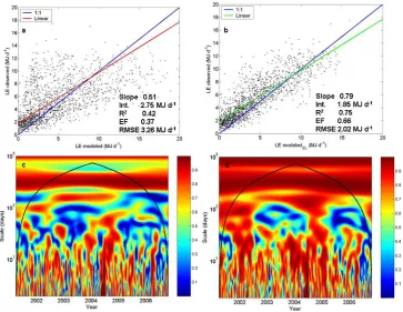
We demonstrate such an approach for model improvement and evaluation by comparing eight years of measured latent heat exchange (LE) from the Tumbarumba flux monitoring site (Leuning et al., 2005) with corresponding predictions from the CABLE model (Kowalczyk et al., 2006), and a CABLE improvement that explicitly accounts for soil and litter layer evaporation (CABLESL – Haverd et al., 2009).
CABLESL represents an improvement in overall model fit
compared to CABLE (Fig. 5a and b), but conventional scat-terplots and associated goodness-of-fit statistics cannot de-termine the times or frequencies when the model has been improved, or how the model can be further improved. (We also note that the daily flux sums are not statistically inde-pendent). The wavelet coherence, similar in mathematical formulation to Pearson’s correlation coefficient, can be used to identify the times and time scales at which two time se-ries are statistically related (Grinsted et al., 2004), and we note that these time series can represent those of measure-ments and models (Fig. 5c and d). Specifically, Grinsted et al. noted that wavelet coherence values above 0.7 (yellow-to-red colours in Fig. 5c and d) represent a significant rela-tionship at the 95% confidence limit.
In the Tumbarumba example, variability in CABLESLis
29 929
930 931 932 933 934 935 936 937 938 939
940
Figure 5: A comprehensive model evaluation framework using measured latent energy flux (LE) from the
Tumbarumba flux monitoring site and corresponding predictions from the CABLE model and model
improvement by adding a soil and litter-layer evaporation scheme (CABLESL). Instantaneous (half-hourly)
observed versus CABLE (a) and CABLESL (b) at the Tumbarumba FLUXNET site for 2001-2006. Some
common evaluation metrics are also displayed. Int = intercept, RMSE = root-mean-square-error. EF = model
efficiency (Meyer and Butler, 1993). The wavelet coherence between observations and the model CABLE (c) and
CABLESL (d) are shown as the full wavelet half-plane. Regions at different time scales (the ordinate)
corresponding to different periods of time (the abscissa) in which the model and measurement are significantly
related at the 95% confidence interval are those that exceed a coherence value of 0.7.
Fig. 5. A comprehensive model evaluation framework using measured latent energy flux (LE) from the Tumbarumba flux monitoring
site and corresponding predictions from the CABLE model and model improvement by adding a soil and litter-layer evaporation scheme (CABLESL). Instantaneous (half-hourly) observed versus CABLE (a) and CABLESL (b) at the Tumbarumba FLUXNET site for 2001– 2006. Some common evaluation metrics are also displayed. Int=intercept, RMSE=root-mean-square-error. EF=model efficiency (Meyer and Butler, 1993). The wavelet coherence between observations and the model CABLE (c) and CABLESL (d) are shown as the full wavelet half-plane. Regions at different time scales (the ordinate) corresponding to different periods of time (the abscissa) in which the model and measurement are significantly related at the 95% confidence interval are those that exceed a coherence value of 0.7.
the measurement record can be identified, and the CABLE model further improved with such a complete “picture”, via the display of wavelet coherence in the wavelet half-plane (i.e. Fig. 5c and d).
5.2 Towards a spatially explicit continental and global scale evaluation of LSMs
LSMs are often evaluated at the site level using EC time series, which can provide detailed information on the per-formance of the temporal dynamics of the model. How-ever, models developed for continental to global applications should be evaluated on the appropriate scale in both time and space. Regional comparisons have largely been neglected partially due to the strong site-by-site focus of flux evaluation to date and partially due to difficulties in “upscaling”. Spa-tially and temporarily explicit maps of carbon fluxes can be derived from empirical models that use FLUXNET measure-ments in conjunction with remotely sensed and/or meteoro-logical data. Different upscaling approaches exist, ranging from simple regression models, to complex machine learning algorithms (Papale and Valentini, 2003; Yang et al., 2007),
The results of such data-oriented models can be used to evaluate process-oriented LSMs operating at regional scales. However, the success of the evaluation depends on whether there is sufficient confidence in the empirical upscaling re-sults, or in other words, if the error of the empirical upscal-ing is substantially smaller than the error of the LSM simu-lations.
[image:8.595.116.480.64.345.2]Table 4. A description of the data-oriented and process-oriented models used to generate catchment scale predictions of GPP across Europe,
which are compared in Fig. 6. Simulations of ORC, LPJmL, BGC, MOD17+, and ANN are from Vetter et al., 2008. MOD17+, ANN, FPA+LC, WBA are calibrated with FLUXNET data.
Acronym Model name Model type Time step Model drivers References
ORC Orchidee Process-oriented Sub-daily Meteorology, Land cover,
soil water holding capacity
(Krinner et al., 2005)
LPJ Lund Potsdam Jena
managed Land (LPJmL)
Process-oriented Daily Meteorology, Land cover,
soil water holding capacity
(Sitch et al., 2003; Bondeau et al., 2007)
BGC Biome-BGC Process-oriented Daily Meteorology, Land cover,
soil water holding capacity
(Thornton, 1998)
MOD17+ Radiation Use efficiency
model
Daily Remote sensing based
FAPAR (MODIS), Meteo-rology, Land cover
(Running et al., 2004)
ANN Artificial Neural
Network
Data-oriented Daily Remote sensing based
FAPAR (Modis), Meteorol-ogy, Land cover
(Papale and Valentini, 2003) updated Vetter et al. (2008)
FPA+LC FAPAR based
Productivity
Assessment+Land Cover
Vegetation type specific regression models between FAPAR and GPP
Annual Remote sensing based
FAPAR (SeaWiFS), Land cover
Jung et al., 2009
WBA Water Balance Approach Upscaling of water use
efficiency
Multi-annual Remote sensing based
LAI (MODIS, CYCLOPES),
Meteorology, Land cover, river runoff data
(Beer et al., 2007), updated
Lund Potsdam Jena managed Land model (LPJmL) showed a reasonable agreement (i.e. highR2)with the different data-oriented results because it has a realistic implementation of crops, in contrast to Biome-BGC and Orchidee, which sim-ulate crops simply as productive grasslands. This treatment appears to be inadequate, as active management and nutrient manipulation differ between a natural grassland and a man-aged agricultural area. Confidence in the data-oriented mod-els is gained by the agreement among independent upscaling approaches.
6 Model-data fusion
Rather than compare model outputs with a particular dataset in order to test or calibrate the model, model-data fusion techniques combines the two sources of information, model and data, into a single product. We define the term “model-data fusion”, sometime called ““model-data assimilation”, to include both state estimation and parameter estimation. State esti-mate involves updating the model state vector PDFs accord-ing to observations, usaccord-ing techniques such as the Kalman fil-ter (Williams et al., 2005), or variational approaches typi-cal with weather forecasting (Courtier et al., 1994). Param-eter estimation involves dParam-etermination of paramParam-eter PDFs using observations. Model-data fusion allows for integrat-ing multiple and different types of data, includintegrat-ing the asso-ciated uncertainties, and for including prior knowledge on model parameters and/or initial state variables. However, the timescales of model processes and observations must over-941
942 943 944 945 946
Figure 6. Model estimates of catchment mean annual GPP for 36 major watersheds in Europe are compared
among different process- and data oriented models. The figure shows the R2 value for each paired comparison
among the 8 models used (see scale bar on right). PCA1 is the first principal component and can be regarded as
the common information content of all models. See Table 4 for abbreviations.
Fig. 6. Model estimates of catchment mean annual GPP for 36
ma-jor watersheds in Europe are compared among different process-and data oriented models. The figure shows the R2 value for each paired comparison among the 8 models used (see scale bar on right). PCA1 is the first principal component and can be regarded as the common information content of all models. See Table 4 for abbre-viations.
lap, otherwise useful information cannot be conveyed to the model from those data by the assimilation scheme.
[image:9.595.309.545.357.517.2]model-data fusion outlined above, the residuals between data and model output after assimilation and the residuals be-tween prior and posterior state and/or parameter values are important information for subsequent steps of model struc-tural development. These residuals help identify model ca-pabilities, particularly those processes which are best con-strained by data. MDF techniques also allow for the propa-gation of uncertainties between the parameter space and the observation space, and thus estimation of model prediction uncertainties, e.g. modelled carbon fluxes (Verbeeck et al., 2006). Below, we first give a brief overview of different MDF techniques with examples to illustrate application and interpretation. We then discuss various problems associated with MDF and suggest solutions.
6.1 Technical implementation
All MDF techniques require certain steps in common. First, the model must be specified, and uncertainties on the model initial states and parameters must be determined a priori. For some algorithms the model uncertainty itself must be esti-mated (e.g. Kalman filter). One approach for setting model errors in Kalman Filter schemes is to ensure that they are set within bounds that are small enough to avoid tracking daily noise in observations, and large enough to shift over weekly-seasonal timescales in response to process signals. Second, data and their uncertainties must be specified. Third, an ob-servation operator must be defined, which links the state vec-tor to the observations, accounting for intermediate processes (e.g. transport processes), requisite scaling and aggregation (e.g. NEE=RE−GPP). Fourth, the optimality condition must
be defined, whether as some sort of cost function to be min-imised, or a joint model-data likelihood. Fifth, the optimal solution is determined. Finally, the posterior probability den-sity functions of the parameters and the state vector must be analysed and interpreted.
The search for an optimal solution and the estimation of uncertainties can be achieved with three different classes of algorithms:
1. “Global search” algorithms, often based on a random generator (Braswell et al., 2005; Sacks et al., 2006). These methods are well adapted for highly non-linear models with multiple minima, but are usually associ-ated with high computational cost because many model evaluations are required. Several algorithms exist, e.g. Metropolis or Metropolis Hastings, genetic algo-rithms.
2. “Gradient-descent” algorithms, following identified di-rections in the parameter space. These methods are highly efficient, but are not best suited for highly di-mensional nonlinear models as they may end up finding local rather than global minima. To determine poste-rior uncertainties, they require the calculation of model
output sensitivity to model parameters (Santaren et al., 2007).
3. “Sequential” algorithms, such as the Kalman filter (Williams et al., 2005; Gove and Hollinger, 2006). These methods process data sequentially, in contrast to the first two classes that treat all observations at once (i.e. batch methods).
Combinations of methods can be successful (Vrugt et al., 2005), such as a global search method to get close to the global minimum, followed by a gradient-descent method to pinpoint the minimum more accurately.
The optimization process for both global search and gradient-descent generally requires the calculation of the mismatch between model outputs (M)and observations (O)
and the mismatch between initial or “prior” (Xp)
parame-ter values and those laparame-ter deparame-termined to be optimal (X) in a Bayesian framework (Eq. 1). The essence of the Bayesian approach is the multiplication of probabilities; in practice the log of the data-model mismatch (log likelihood) is summed with the log of the prior probabilities. Both mismatches are weighted according to confidence on observations (R ma-trix) and prior knowledge about parameter error covariance (P matrix). The R matrix may contain different kinds of data, which are matched by their error covariances. The P matrix is crucial because it allows the consistent combination of dif-ferent kinds of data into one formulation of the cost function.
H is the observation operator, which relates the model state vector to the observations. The data-model and parameter mismatches define the objective or cost function,J, used in many batch optimisation methods (Lorenc, 1995):
J=1/2[(H M−O)TR−1(H M−O)+(X−Xp)TP−1(X−Xp)] (1)
There are similarities betweenJand the Kalman gain (K)
used in Kalman filters. K is used to adjust the model fore-cast (Mf)to generate an optimal analysis (Ma)based on the differences between model and observations, and the confi-dence in model (P matrix) and observations (R matrix):
K=PfHT(H PfHT +R)−1 (2)
Ma=Mf +K(O−H Mf) (3)
The model error covariance matrix (P)is updated dynam-ically in the Kalman filter as observations are assimilated.
The cost function defined above (Eq. 1) is commonly used when the error is known or assumed to be Gaussian, but other options are possible. For example, the sum of absolute devia-tions rather than squared deviadevia-tions between data and model form the likelihood when data errors are exponential, reduc-ing the influence of outliers in the cost function compared to Eq. (1). The choice of cost function is an important one; an optimization intercomparison by Trudinger et al. (2007) found significantly more variation in estimated parameters due to definition of the cost function than choice of mization technique. Another important choice in the opti-misation is whether to include all parameters at once at the risk that interactions among parameters yield big uncertain-ties and a poor convergence of the algorithm. Optimizing for just a small set of pre-identified parameters may not include key processes (Wang et al., 2001; Reichstein et al., 2003), and in fact is mathematically equivalent to holding constant those parameters not optimized.
6.2 Error estimations: random and systematic error There are two important differences between random and systematic measurement errors. First, whereas statistical analyses can be used to estimate the size of random errors (Lasslop et al., 2008), systematic errors are difficult to detect or quantify in data-based analyses (Moncrieff et al., 1996); but see Lee (1998). Second, random errors in data will in-crease the uncertainty in data-model fusion parameter esti-mates and model predictions, but should not bias the poste-rior estimates. Systematic errors in data, on the other hand, are more insidious in that, if not corrected first, they will di-rectly result in biased posteriors, see Lasslop et al. (2008) for an example.
However, as noted above, systematic errors will be iden-tified by the multiple-constraints approach via model-data mismatch. On the other hand, large random errors in obser-vations, while increasing uncertainties of the estimated pa-rameters, decrease the usefulness of the model-data fusion approach because the analysis errors are not much reduced from the original background (prior) errors.
Estimates of prior values and errors on model param-eters is usually undertaken using literature values, global databases (http://www.try-db.org/, Wright et al., 2004) and expert estimation. This critical task partly conditions the re-alism of the inverse estimates. The role of the user in set-ting parameter and model errors requires careful inspection of posterior distributions to determine if MDF has succeeded (see Sect. 6.6).
6.3 The initial condition problem
Correct estimates of both vegetation and soil carbon pools constitute an initial condition problem of significant rele-vance in those LSMs with dynamic biogeochemical (BGC) modelling. The current best practice in LSMs applied
glob-947
948
949 950
[image:11.595.310.545.62.216.2]951
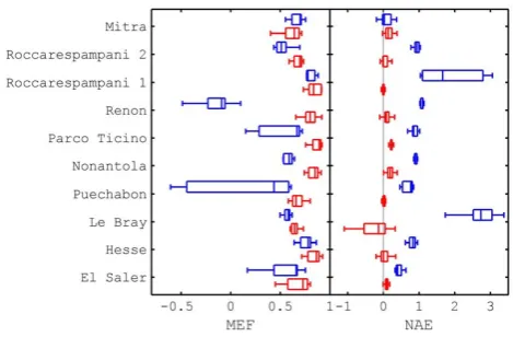
Figure 7 CASA model performance statistics for NEP at ten eddy covariance sites is higher in relaxed steady state approaches (red) than in cases considering ecosystems in equilibrium for model optimization (blue) (MEF – model efficiency; and NAE – normalized average error) (Carvalhais et al., 2008).
31
Fig. 7. CASA model performance statistics for NEP at ten eddy
covariance sites is higher in relaxed steady state approaches (red) than in cases considering ecosystems in equilibrium for model op-timization (blue) (MEF – model efficiency; and NAE – normalized average error) (Carvalhais et al., 2008).
ally is to use spin-up routines until the C cycle is in equi-librium with pre-industrial climate, followed by transient in-dustrial climate, atmospheric CO2 and N deposition runs
(Churkina et al., 2003; Thornton et al., 2002; Morales et al., 2005), and then impose historical land-use change and management. The initialization process is often prescribed until ecosystem atmosphere fluxes are in equilibrium, which may lead to overestimation of both soil (Pietsch and Hase-nauer, 2006; Wutzler and Reichstein, 2007) and vegetation pools, consequently increasing total respiration (RE). The
equilibrium assumption may be criticised as not being fully applicable to natural ecosystems. In BGC-model-data fusion approaches, both empirical as well as process-based method-ologies have been proposed to address these issues (Santaren et al., 2007; Carvalhais et al., 2008; Luo et al., 2001; Pietsch and Hasenauer, 2006). In ecosystems far from equilibrium, model parameter uncertainties and biases can be avoided by relaxing the steady state assumption, i.e. optimizing the ini-tial conditions of C pools (Carvalhais et al., 2008), which reduces model estimates uncertainties in upscaling exercises. As an example, in Fig. 7 we show CASA model performance statistics for estimated net ecosystem production compared against data from ten EC sites. We compared performance with spun-up initial conditions (i.e. steady state) against an approach that relaxed the steady state assumption. Perfor-mance after parameter optimisation was higher using the re-laxed approach rather than one that considered the system in equilibrium.
32
952
[image:12.595.69.270.78.604.2]953
954
955
956
957
Figure 8 Results from a genetic algorithm (GA) applied to parameter estimation in the DALEC model as part of
the REFLEX project (Fox et al., in press). Synthetic, noisy and sparse data were supplied to the GA. As the
calculations proceeded, the current best estimate of parameters and the corresponding cost function were saved,
and values of the cost function and selected parameters (p1, p10, p12) are shown here.
32
952
953
954
955
956
957
Figure 8 Results from a genetic algorithm (GA) applied to parameter estimation in the DALEC model as part of
the REFLEX project (Fox et al., in press). Synthetic, noisy and sparse data were supplied to the GA. As the
calculations proceeded, the current best estimate of parameters and the corresponding cost function were saved,
and values of the cost function and selected parameters (p1, p10, p12) are shown here.
Fig. 8. Results from a genetic algorithm (GA) applied to parameter
estimation in the DALEC model as part of the REFLEX project (Fox et al., 2009). Synthetic, noisy and sparse data were supplied to the GA. As the calculations proceeded, the current best estimate of parameters and the corresponding cost function were saved, and values of the cost function and selected parameters (p1, p10, p12) are shown here.
for woody biomass constraints, for which forest inventories as well as synthesis activities are key contributors (Luyssaert et al., 2007). Disturbance and management history (Thorn-ton et al., 2002) are additional factors that control the initial condition of any particular simulation. There are clearly con-siderable challenges related to generating the historical data and including historical and current management regimes. 6.4 Equifinality
An important issue in parameter estimation is equifinality, where different model representations, through parameters or model structures, yield similar effects on model outputs, and so can be difficult to distinguish (Medlyn et al., 2005; Beven and Freer, 2001). Such correlations imply that quite differ-ent combinations of model parameters or represdiffer-entations can give a similar match of model outputs to observations. This problem is particularly relevant to observations of net fluxes, which on their own may not provide enough information to constrain parameters associated with the component gross fluxes. Further, the associated uncertainties in a posteriori regional upscaling are significant and variable in space and time (Tang and Zhang, 2008) Equifinality in parameter esti-mation is illustrated in Fig. 8, which shows the results of a genetic algorithm applied to the DALEC model (Williams et al., 2005), as part of the REFLEX project (Fox et al., 2009). The cost function decreased quickly at first, but after about 100 iterations of the genetic algorithm there was only grad-ual further improvement, yet the values of some parameters varied significantly after this point (Fig. 8). Addressing equi-finality requires identification of covariances between param-eter estimates, the use of multiple, orthogonal data sets, and testing a variety of cost functions to constrain unidentifiable parameters. Thus, it is critical to assess whether the available observations can adequately constrain the model parameters or whether more information is required.
6.5 Parameter validation and uncertainty propagation Estimated parameters should always be interpreted with great care. Posterior values are not always directly inter-pretable (i.e. in a biological sense) due to equifinality (see above) or to compensating mechanisms related to model de-ficiencies/biases. In addition, simplified model structures re-quire aggregated parameters (e.g. aVcmax– maximum rate of
carboxylation – value of a “big leaf”) that will always be dif-ferent from observed parameter values (e.g. determined from measurements ofVcmaxon an individual leaf). Nevertheless,
comparison with independent real measured parameter val-ues is an important part of the analysis and validation pro-cess. For example, Santaren et al. (2007) successfully com-pared their estimated Vcmax with estimates from leaf-level
measurements (their Fig. 7).
A benefit of most model-data fusion approaches is to es-timate parameter uncertainties and the corresponding model
output uncertainties. The outcome of the MDF is a set of pa-rameter PDFs which can then be used to generate an ensem-ble of model runs, using time series of climate forcing data. As an example, we generated synthetic, noisy and sparse data from the DALEC model using nominal parameters, and sup-plied these to an Ensemble Kalman filter (Williams et al., 2005) for parameter estimation. The outputs of the EnKF were parameter frequency distributions that indicated the statistics of the retrieved parameters generated by inverting the observations. In Fig. 9 we show the retrieved PDFs for the turnover rates for four C pools, which can be compared to the true parameter values (vertical lines), and the prior pa-rameter values, which are represented by the width of the x-axes. The process of estimating confidence intervals of model states and predictions is highly dependent on the prior estimates of parameter (and model) error, as shown in the REFLEX experiment (Fox et al., 2009). We are still learning how to properly quantify confidence intervals on parameter and state analyses.
6.6 How to assess a model-data fusion scheme
A first step to testing if MDF approaches are effective is to use synthetic data, where the underlying “true” state of the system and model parameters are known. A synthetic truth is generated by running the model with given parameters, noise is added, and data are thinned. These data are provided to the MDF scheme to test estimation of parameters and retrieval of C fluxes, all of which are known (Fig. 9). A second step is to examine posterior parameter distributions relative to pri-ors. Have parameters been constrained? Is there evidence that parameter priors were correct? For example, in the syn-thetic case shown in Fig. 9 it is clear that turnover rates of foliage and soil organic matter were better constrained by NEE data, with PDFs concentrated around the true param-eter values used to generate the synthetic data. Posterior turnover rates for fine roots and wood are barely different from the priors, with broad distributions spanning the prior range. A third step is to check model residuals on NEE (or any other observations), to see if they are Gaussian and not autocorrelated, a typical hypothesis of Bayesian approaches (see above). If multiple data time series are used, are they all consistent with the model, or do they reveal potential bi-ases in data or model (Williams et al., 2005)? It is useful to iterate the optimization process from a different starting point (initial conditions) to see if the posteriors are similar. Testing different assumptions in the MDF is also useful, for instance, uniform versus Gaussian priors, altered model error estimates in KF schemes etc.
6.7 Spatial and temporal parameter variability
With increasing FLUXNET data availability over a wide range of ecosystems, model-data fusion approaches can im-prove our understanding and process representation ability
33 959
[image:13.595.310.545.62.254.2]960 961 962 963 964 965 966 967
Figure 9. Parameter retrieval from a synthetic experiment using the DALEC model (Williams et al., 2005).
Synthetic, noisy and sparse data generated from DALEC were supplied to an Ensemble Kalman filter (Williams
et al., 2005) for parameter estimation. “True” parameter values for turnover rates of foliage, stem wood, fine
roots and soil organic matter are shown by the red lines. The frequency distributions indicate the statistics of the
retrieved parameters generated by inverting the observations. The x-axis limits indicate the spread of the prior
estimates for each parameter.
Fig. 9. Parameter retrieval from a synthetic experiment using the
DALEC model (Williams et al., 2005). Synthetic, noisy and sparse data generated from DALEC were supplied to an Ensemble Kalman filter (Williams et al., 2005) for parameter estimation. “True” pa-rameter values for turnover rates of foliage, stem wood, fine roots and soil organic matter are shown by the red lines. The frequency distributions indicate the statistics of the retrieved parameters gen-erated by inverting the observations. The x-axis limits indicate the spread of the prior estimates for each parameter.
at regional and global scales. So far most biogeochemical models use the concept of “plant functional type” to repre-sent the ecosystem diversity, with typically 6 to 15 classes. Whether the associated parameters or process representa-tions are generic enough to apply across climate regimes, species differences, as well as large temporal domains or whether they should be refined are critical questions that FLUXNET data can help resolve.
6.7.1 Temporal variability
For a prognostic model to be useful, dynamic processes must be represented within the model, and parameters must be constant in time. If there is evidence that parameters vary over time (Hui et al., 2003; Richardson et al., 2007), it means the parameters are sensitive and that some component of model structure is missing. The relevant structure must be included in the model for it to have prognostic value. Like-wise, if there is no evidence that parameters vary, then they are shown to be insensitive. The estimation of process pa-rameters in variable conditions over time is likely to give new insights in processes that are poorly understood (Santaren et al., 2007). Building on the work of Santaren et al. (2007), we optimised the ORCHIDEE biogeochemical model against eddy covariance data to retrieve the year-to-year variabil-ity of maximum photosynthetic capacvariabil-ity (Vcmax).
968 969 970 971 972 973 974 975
Figure 10 Some results from the optimisation of 18 parameters of the ORCHIDEE model at 4 temperate
needleleaf forest sites for several years: 2 years at le Bray (BX) and Aberfeldy (AB) and 4 years at Tharandt
(TH) and Weilden (WE). Green is prior ORCHIDEE model, red is optimised model, black are the data.One
parameter set is optimized each year using NEE, latent, sensible and net radiation fluxes (using half hourly
values, see Santaren et al. 2007). Upper panels show the model-data fit (daily values and mean diurnal cycle
during the growing season) while the lower panel shows the estimated Vcmax parameter values for each sites and
each year: values a reported with respect to the prior value.
34
Fig. 10. Some results from the optimisation of 18 parameters of the
ORCHIDEE model at 4 temperate needleleaf forest sites for sev-eral years: 2 years at le Bray (BX) and Aberfeldy (AB) and 4 years at Tharandt (TH) and Weilden (WE). Green is prior ORCHIDEE model, red is optimised model, black are the data. One parameter set is optimized each year using NEE, latent, sensible and net ra-diation fluxes (using half hourly values, see Santaren et al., 2007). Upper panels show the model-data fit (daily values and mean diur-nal cycle during the growing season) while the lower panel shows the estimated Vcmax parameter values for each sites and each year: values a reported with respect to the prior value.
Tharandt sites suggest there area additional processes related to productivity not captured by ORCHIDEE, and possibly linked to the N cycle (Fig. 10). Similarly, Reichstein et al. (2003) studied drought events by estimating the seasonal time course of parameters of the PROXEL model using eddy covariance carbon and water fluxes at Mediterranean ecosys-tems.
6.8 Spatial variability
The concept of plant functional type (PFT) simplifies the rep-resentation of ecosystem functioning and groups model pa-rameter values estimated at site level. However, inter-site parameter variability for analogous PFTs show limitations of such a regionalization approach (Ibrom et al., 2006; van Dijk et al., 2005). Parameters that show large between-site but low temporal variability should be used to help define more realistic PFTs than are currently applied. The spatial varia-tion in parameters should be explicable on the basis of exter-nal drivers such as climatic, topographic or geological vari-ability. Model parameter regionalization approaches usually build on remotely sensed variables as model drivers which are providing a basis for the extrapolation of spatial patterns, but the quantification of the FLUXNET representativeness and heterogeneity is fundamental to assess the upscaling po-tential of both model parameters and observed processes.
6.9 Evaluation of model deficiencies and benchmarking One of the major interests of assimilation techniques for modellers is in the potential to highlight model deficiencies. For this objective, being able to include all sources of un-certainty within a rigorous statistical framework represents a critical advantage. Abramowitz et al. (2005, 2008, 2007) used artificial neural networks (ANN) linking meteorological forcing and measured fluxes to provide benchmarks against which to assess performance of several LSMs. Performance of the ANNs was generally superior to that of the LSMs, which produced systematic errors in the fluxes of sensible heat, water vapour and CO2 at five test FLUXNET sites.
These errors could not be eliminated through parameter op-timization and it appears that structural improvements in the LSMs are needed before their performance matches that of the benchmark ANNs. Predictions using LSMs may be sat-isfactory in some parts of bioclimatic space and not in others. Abramowitz et al. (2008) used self-organizing maps to divide climate space into a set distinct regions to help identify con-ditions under which model bias is greatest, thereby helping with the “detective work” of model improvement.
With conventional model-data evaluation (e.g. RMSE analyses) there is always the risk of over-interpretation of a particular model-data mismatch, that only reflects poor pa-rameter calibrations. The details of these outcomes are prob-ably only relevant to a given model structure and thus cannot be extrapolated to other models. As an example, Fig. 10 il-lustrates the difficulty of one model to properly capture the amplitude of both the seasonal cycle and the summer diurnal cycle of NEE (and not for the latent heat flux). Note that the issue of temporal and spatial variability, discussed above, is also relevant to this objective. However, a caution with any parameter optimization process is not to correct for model biases with unrealistic parameter values, by carefully evalu-ating the posterior parameter estimates. Model failure after optimisation identifies inadequate model structure, which ul-timately leads to improvements in process representation and increased confidence in the model’s projections.
7 Conclusions
Our vision for the future includes: (1) identifying and funding critical new locations for FLUXNET towers in poorly studied biomes, for instance in tropical croplands; (2) nesting EC towers within the regional footprints of tall towers that sample the CO2 concentration of the planetary
boundary layer (Helliker et al., 2004) to assist upscaling; (3) linking EC towers effectively with the atmospheric col-umn CO2measurements generated by the satellites OCO and
GOSAT, expected from late 2009 (Feng et al., 2008); (4) continued linkage to optical products from remote sensing, as these provide critical information on canopy structure and phenology (Demarty et al., 2007); (5) use of plant functional traits database to identify more realistic priors and to vali-date posteriors in the data assimilation process (Luyssaert et al., 2007). Full exploitation of this vision is dependent on model-data fusion. Atmospheric transport models are criti-cal for linking land surface exchanges to CO2concentration
measurements from (2) and (3). Radiative transfer models are vital for properly assimilating the raw optical informa-tion from remote sensing (Quaife et al., 2008).
We have identified five major model-data fusion chal-lenges for the FLUXNET and LSM communities to tackle, for improved assessment of current and future land surface exchanges of matter and energy:
– To determine appropriate use of current data and to ex-plore the information gained in using longer time series regarding future prediction. What can be learned from assimilating 10+ years of EC data?
– To avoid confounding effects of missing processes in model representation on parameter estimation.
– To assimilate more data types (e.g. pools/stocks of car-bon, earth observation data) and to define improved ob-servation operators. It would be valuable to determine which biometric time series would best complement EC data at FLUXNET sites.
– To fully quantify uncertainties arising from data bias, model structure, and estimates of initial conditions. We believe that MDF with multiple independent data time series will best identify bias, and recommend a multi-site test of this idea.
– To carefully test current model concepts (e.g. PFTs) and guide development of new concepts. FLUXNET data can be used to determine whether parameters need to vary continuously in space in response to some remotely sensed trait, following approaches applied, for instance, by Williams et al. (2006). Thus, FLUXNET data can be used to challenge and enrich the PFT approach, possibly leading to a redefinition of PFTs.
Acknowledgements. NERC funded part of this work through the
CarbonFusion International Opportunities grant. We acknowledge the assistance received from M. Detto, G. Abramowitz and D. Santaren in the preparation of this manuscript.
Edited by: B. Medlyn
References
Abramowitz, G.: Towards a benchmark for land surface models, Geophys. Res. Lett., 32, L22702, doi:10.1029/2005GL024419, 2005.
Abramowitz, G. and Pitman, A.: Systematic bias in land surface models, J. Hydrometeorol., 8, 989–1001, 2007.
Abramowitz, G. and Gupta, H.: Toward a model space and
model independence metric, Geophys. Res. Lett., 35, L05705, 10.1029/2007GL032834, 2008.
Aubinet, M., Grelle, A., Ibrom, A., Rannik, U., Moncrieff, J., Fo-ken, T., Kowalski, A. S., Martin, P. H., Berbigier, P., Bernhofer, C., Clement, R., Elbers, J., Granier, A., Grunwald, T., Mor-genstern, K., Pilegaard, K., and Rebmann: Estimates of the an-nual net carbon and water exchange of forests: the EUROFLUX methodology, Adv. Ecol. Res., 30, 113–175, 2000.
Baldocchi, D., Falge, E., Gu, L. H., Olson, R., Hollinger, D., Running, S., Anthoni, P., Bernhofer, C., Davis, K., Evans, R., Fuentes, J., Goldstein, A., Katul, G., Law, B., Lee, X. H., Malhi, Y., Meyers, T., Munger, W., Oechel, W., U, K. T. P., Pilegaard, K., Schmid, H. P., Valentini, R., Verma, S., Vesala, T., Wilson, K., and Wofsy, S.: FLUXNET: A new tool to study the temporal and spatial variability of ecosystem-scale carbon dioxide, water vapor, and energy flux densities, B. Am. Meteor. Soc., 82, 2415– 2434, 2001.
Baldocchi, D. D.: Assessing the eddy covariance technique for evaluating carbon dioxide exchange rates of ecosystems: past, present and future, Glob. Ch. Biol., 9, 479–492, 2003.
Beer, C., Reichstein, M., Ciais, P., Farquhar, G. D., and Papale, D.: Mean annual GPP of Europe derived from its water balance, Geophys. Res. Lett., 34, L05401, doi: 10.1029/GL029006, 2007. Beven, K. and Freer, J.: Equifinality, data assimilation, and uncer-tainty estimation in mechanistic modelling of complex environ-mental systems using the GLUE methodology, J. Hydrol., 249, 11–29, 2001.
Bonan, G. B.: Land atmosphere CO2 exchange simulated by a
land-surface process model coupled to an atmospheric general-circulation model, J. Geophys. Res.-Atmos., 100, 2817–2831, 1995.
Bonan, G. B.: Forests and Climate Change: Forcings, Feedbacks, and the Climate Benefits of Forests, Science, 320, 1444–1449, doi:10.1126/science.1155121, 2008.
Bondeau, A., Smith, P. C., Zaehle, S., Schaphoff, S., Lucht, W., Cramer, W., and Gerten, D.: Modelling the role of agriculture for the 20th century global terrestrial carbon balance, Glob. Change Biol., 13, 679–706, 2007.