Reservoir Operation During Droughts

RESERVOIR OPERATION DURING DROUGHTS

A. B. Dariane

Department of Civil Engineering, KN Toosi University of Technology PO Box 11365-1866, Tehran, Iran, [email protected]

(Received: May 8, 2002 – Accepted in Revised Form: August 11, 2003)

Abstract Drought is an inevitable part of the world’s climate. It occurs in wet as well as in dry regions. Therefore, planning for drought and mitigating its impacts is essential. In this study, a hedging rule is developed using the zero/one mixed integer-programming approach. Furthermore, some procedures are introduced to ease the computational burden inherent in integer programming. Hedging rules are developed using three, two, and one-year historical droughts. Moreover, yield model (YM) along with the standard operating policy (SOP) are also formulated for comparison purposes. Simulations are carried out using 40 years of monthly historical data along with 20 series of synthetically generated inflows of the same length. The Karadj reservoir located in the northwest of Tehran is the major source of the capital’s municipal water supply. It also provides a substantial portion of the irrigation demand of the Karadj Valley. Synthetic data are generated using single and multi-variate autoregressive modeling approaches. Models are compared using important reservoir operation criteria including reliability, resiliency, and vulnerability. As compared to the well-known SOP model, it is noticed that the application of the hedging rule and the yield model substantially reduces the system reliability as well as it’s vulnerability, however it increases the resiliency. Moreover, hedging rules developed using longer drought periods tend to have lower vulnerability and reliability, and higher resiliency.

Key Words Drought, Hedging Rule, Reservoir Management, Reservoir Operation, Karadj Reservoir, Yield Model, Zero/One Programming, Water Deficit Management

ﻩﺪﻴﮑﭼ

ﻩﺪﻴﮑﭼ

ﻩﺪﻴﮑﭼ

ﻩﺪﻴﮑﭼ

ﻲﻣﺭﺎﻤﺷﻪﺑ ﺏﺁ ﻊﺑﺎﻨﻣ ﻱﺰﻳﺭ ﻪﻣﺎﻧﺮﺑﺭﺩ ﻲﺳﺎﺳﺍ ﺕﺎﻋﻮﺿﻮﻣ ﺯﺍﯽﮑﻳ ﻲﻟﺎﺴﻜﺸﺧ ﻩﺯﻭﺮﻣﺍ ﺪﻳﺁ

.

ﻪﮑﻳﺭﻮﻄﺑ

ﻲﻤﻧﻭﻩﺩﻮﺑﺺﻗﺎﻧﻲﻟﺎﺴﻜﺸﺧ ﻥﺩﻮﻤﻧﻅﺎﺤﻟﻥﻭﺪﺑ ﻪﻨﻴﻣﺯﻦﻳﺍ ﺭﺩﻱﺰﻳﺭﻪﻣﺎﻧﺮﺑﻪﻧﻮﮔﺮﻫ

ﺕﻼﻀﻌﻣﻱﻮﮕﺨﺳﺎﭘ ﺪﻧﺍﻮﺗ

ﺪﺷﺎﺑﺎﻫﻲﻟﺎﺴﮑﺸﺧﺮﺛﺍﺭﺩﻩﺪﺷﺩﺎﺠﻳﺍ

.

ﻨﺘﺟﺍﻭﻲﻌﻴﺒﻃﻩﺪﻳﺪﭘﮏﻳﻲﻟﺎﺴﮑﺸﺧﻲﻓﺮﻃﺯﺍ ﻲﺘﺣﻲﻳﺍﻮﻫﻭﺏﺁﺮﻳﺬﭘﺎﻧﺏﺎ

ﻲﻣﻥﺎﻬﺟﻥﺍﺭﺎﺑﺮﭘﻱﺎﻫﺶﺨﺑﺭﺩ ﺪﺷﺎﺑ

.

ﻱﺭﻭﺮﺿﻭﻡﺯﻻﻥﺁﺕﺍﺮﺛﺍﻦﺘﺳﺎﮐﻭﻥﺁﺎﺑﻪﻠﺑﺎﻘﻣﻱﺍﺮﺑﻱﺰﻳﺭﻪﻣﺎﻧﺮﺑﻦﻳﺍﺮﺑﺎﻨﺑ

ﻲﻣ ﺪﺷﺎﺑ

.

ﻲﻣﻩﺩﺎﻔﺘﺳﺍ ﻱﺪﻨﺑﻩﺮﻴﺟ ﯼﺎﻬﻟﺪﻣ ﺯﺍ،ﺏﺁﺩﻮﺒﻤﮐ ﺕﺍﺮﺛﺍ ﻦﺘﺳﺎﮐ ﻱﺍﺮﺑﻲﻧﺎﺳﺮﺑﺁ ﻱﺎﻫﻢﺘﺴﻴﺳ ﺭﺩ ﺪﻨﻨﮐ

.

ﻦﻳﺍ

ﻲﻣ ﺮﻳﺬﭘﻪﻴﺟﻮﺗ ﻲﺘﻗﻭ ﻞﻤﻋ ﻪﮐ ﺪﺷﺎﺑ

ﻱﺎﻫﺩﻮﺒﻤﮐ ﻪﮑﻳﺭﻮﻄﺑ ،ﺪﻨﺷﺎﺑ ﻲﻄﺧﺮﻴﻏ ﺕﺭﺎﺴﺧ ﻊﺑﺍﻮﺗ ﯼﺍﺭﺍﺩ ﺏﺁ ﻑﺭﺎﺼﻣ

ﺪﻧﻮﺷﺚﻋﺎﺑﺍﺭﻱﺮﺘﺸﻴﺑﻲﻠﻴﺧﺕﺍﺭﺎﺴﺧﺮﺘﮔﺭﺰﺑ

. ﻭﺩﻪﺘﺴﺴﮔ ﻱﺪﻨﺑﻩﺮﻴﺟﻱﺯﺎﺳﻪﻨﻴﻬﺑﻝﺪﻣﮏﻳﺯﺍﻖﻴﻘﺤﺗﻦﻳﺍﺭﺩ

ﺪﺷﻩﺩﺎﻔﺘﺳﺍﮏﺸﺧﻩﺭﻭﺩﮏﻳﺭﺩﻥﺰﺨﻣﺖﻳِﺮﻳﺪﻣﯼﺍﺮﺑﻩﺪﺷﺡﻼﺻﺍﻱﺍﻪﻠﺣﺮﻣ

. ﻪﺑﻪﮐﻩﺪﺷﺡﻼﺻﺍﺵﻭﺭﻦﻳﺍﺭﺩ

ﮔ ﻪﺑ ﻡﺎﮔ ﺕﺭﻮﺻ

ﻲﻣﻞﺣ ﻡﺎ

ﺩﺭﺍﺩ ﺩﻮﺟﻭﺮﺘﺸﻴﺑ ﻱﺎﻬﻟﺎﺳ ﺩﺍﺪﻌﺗﯼﺍﺮﺑ ﻱﺪﻨﺑ ﻩﺮﻴﺟﻝﺪﻣ ﯼﺍﺮﺟﺍ ﻥﺎﮑﻣﺍ ،ﺩﻮﺷ

.

ﻥﺎﻣﺯ

ﻲﻣ ﺶﻫﺎﮐﻱﺍ ﻪﻈﺣﻼﻣ ﻞﺑﺎﻗ ﺭﻮﻃﻪﺑ ﺰﻴﻧ ﻩﺪﺷﺡﻼﺻﺍ ﻝﺪﻣ ﯼﺍﺮﺟﺍ ﺪﺑﺎﻳ

. ﺪﺳ ﻢﺘﺴﻴﺳﯼﻭﺭ ﺮﺑﻝﺪﻣ ﯼﺍﺮﺟﺍﺞﻳﺎﺘﻧ

ﺪﺷﺡﻼﺻﺍﻝﺪﻣ،ﻪﺑﺎﺸﻣﻡﻭﺩﻪﻠﺣﺮﻣﯼﺪﻨﺑﻩﺮﻴﺟﻱﺎﻫﻩﺭﻭﺩﺩﺍﺪﻌﺗﯼﺍﺯﺍﻪﺑﻪﮐﺩﺍﺩﻥﺎﺸﻧﺝﺮﮐﻲﻧﺰﺨﻣ

ﺎﺑﻪﺴﻳﺎﻘﻣﺭﺩﻩ

ﻟﻭﺍﻝﺪﻣ ِﻴ ﻲﻣﻥﺎﺸﻧﯼﺮﺘﺑﻮﻠﻄﻣﺞﻳﺎﺘﻧﻪ ﺪﻫﺩ

.

ﻲﻣﺮﺘﺸﻴﺑﻥﺁﻱﺪﻨﺑﻩﺮﻴﺟﻥﻭﺪﺑﻱﺎﻫﻩﺭﻭﺩﺩﺍﺪﻌﺗﻪﮑﻨﻳﺍﻲﻨﻌﻳ ﺪﺷﺎﺑ

.

ﻦﻳﺍﺎﻣﺍ

ﻪﻠﺣﺮﻣﻱﺪﻨﺑﻩﺮﻴﺟﻱﺎﻫﻩﺭﻭﺩﺩﺍﺪﻌﺗﺶﻳﺍﺰﻓﺍﺎﺑﺖﻴﻌﺿﻭ ۲

ﻲﻣﺲﮑﻋﺮﺑ ﺩﻮﺷ

. ﮏﺸﺧﻱﺎﻫﻩﺭﻭﺩﻱﺍﺮﺑﻝﺪﻣﻱﺍﺮﺟﺍ

ﻲﻣﻥﺎﺸﻧﻪﻟﺎﺳﻪﺳﻲﻟﺍﮏﻳ

ﻩﺭﻭﺩﺶﻳﺍﺰﻓﺍﺎﺑﻪﮐﺪﻫﺩ

ﺩﺎﻤﺘﻋﺍﻥﻮﭽﻤﻫﻲﺑﺎﻳﺯﺭﺍﯼﺎﻫﺭﺎﻴﻌﻣ،ﻝﺪﻣﺭﺩﻲﻟﺎﺴﮑﺸﺧ ﻱﺮﻳﺬﭘ

ﻲﻣﺶﻳﺍﺰﻓﺍﻱﺮﻳﺬﭘﺖﺸﮔﺮﺑﻭﻪﺘﻓﺎﻳﺶﻫﺎﮐﯼﺮﻳﺬﭘﺐﻴﺳﺁﻭ ﺪﺑﺎﻳ

.

ﯽﺳﺭﺮﺑﻭﻞﻴﻠﺤﺗﺩﺭﻮﻣﻒﻠﺘﺨﻣﻱﺎﻫﻪﺒﻨﺟﺯﺍﻝﺪﻣ

ﺖﺳﺍﻩﺪﻳﺩﺮﮔﻪﺴﻳﺎﻘﻣﺩﺭﺍﺪﻧﺎﺘﺳﺍﯼﺭﺍﺩﺮﺑﻩﺮﻬﺑﻝﺪﻣﻭﻲﻫﺪﺑﺁﻝﺪﻣﮏﻳﺎﺑﻭﻪﺘﻓﺮﮔﺭﺍﺮﻗ

.

ﻲﻣﻥﺎﺸﻧﺞﻳﺎﺘﻧ

ﻝﺪﻣﻪﮐﺪﻫﺩ

ﻨﺑ ﻩﺮﻴﺟ

ﺩﺭﺍﺩ ﻲﻟﺎﺴﮑﺸﺧ ﺯﺍﻲﺷﺎﻧﺕﺍﺭﺎﺴﺧ ﺶﻫﺎﮐﺭﺩﻲﺳﻮﺴﺤﻣ ﯼﺮﺗﺮﺑ ﻱﺪ

.

ﺭﺎﮑﺑ

ﻲﻣﯼﺭﺍﺰﺑﺍﻦﻴﻨﭼﻱﺮﻴﮔ ﺪﻧﺍﻮﺗ

ﺪﻳﺎﻤﻨﺑﺐﺳﺎﻨﻣﺕﺎﻤﻴﻤﺼﺗﺫﺎﺨﺗﺍﺭﺩﻥﺍﺮﻳﺪﻣﻪﺑﺏﺁﻥﺍﺮﺤﺑﻊﻗﺍﻮﻣﺭﺩﻲﻧﺎﻳﺎﺷﮏﻤﮐ

.

1.

Hedging is based on the fact that having more frequent droughts of lower intensity is preferred

words, losses due to droughts are not linear. On the other hand, uncertainties on the future events prevent us from a perfect allocation of resources during a drought. Therefore, it is inevitable to search for models that could help us in these situations. These models must rely on the trend of the past events. They usually consist of two types; optimization and simulation. Simulations are typically used to study and verify the results of optimization models.

Despite of the fact that it is an inevitable part of today’s world, there has been less effort and research on the planning of resources during droughts. Drought is a very general term with no unique definition. However, in water resources we may define it as a situation in which due to lower river flows, demands are not met. Alike to its definition, the extension and variety of studies carried out are numerous. In this paper, we have focused on the approaches that are used to manage a reservoir system during some critical drought periods. Hedging is an approach that is used for reservoir operation during droughts. Shih and Revelle [1] introduced and developed a continuous hedging rule for a single reservoir operation. They used a Zero/One programming to linearize the nonlinear functions. Dariane [2] used a different procedure to solve the nonlinear functions and showed that the solution algorithm employed by Shih and Revelle [1] is not efficient. He also proposed a revision on the objective function to include the importance of different values of the water released in different periods. Bayazit and Unal [3] investigated the impact of hedging on a reservoir operation. They concluded that the reliability and vulnerability of the system is reduced when hedging is applied.

Srinvasan and Philipose [4] and [5] studied the sensitivity of a system to the changes in hedging thresholds. Shih and Revelle [6] extended their previous work and developed a discrete hedging rule. Neelakantan and Pundarikanthan [7] studied the discrete hedging rule by optimization and simulation models.

2. MODEL DEVELOPMENT

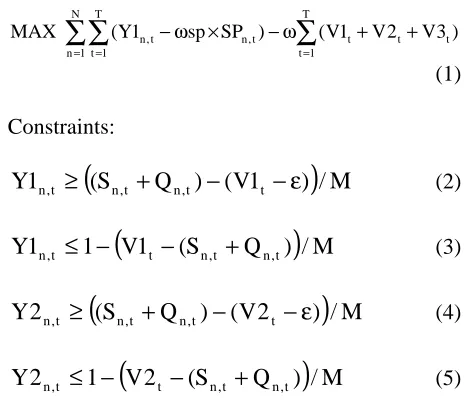
In this paper, we employed the discrete hedging model originally developed by Shih and Revelle [6]. Our objective is to develop a practical reservoir operation model during drought periods. Figure 1 shows the model with two hedging levels. Application of the model developed by Shih and Revelle [6] indicated very high computer execution time and memory utilization. In fact, for some cases of their example, we never reached a solution within acceptable time consumption. These are the cases where the phase 2 frequencies are low enough to force the model to extensively search for optimal solutions. Therefore, we moved the spilling constraint into the objective function. This eliminated 36 zero/one variables responsible to control spills from the reservoir, resulting in substantial reduction of computer time and memory utilization. Despite these changes, it was not yet possible to reach any solution using a Pentium II computer. The followings are the revised objective function and constraints of the model. Objective:

∑

∑∑

= = =

+ + ω

− × ω

− T

1 t

t t t N

1 n

T

1 t

t , n t

,

n sp SP ) (V1 V2 V3)

1 Y ( MAX

(1)

Constraints:

(

(

S

Q

)

(

V

1

)

)

/

M

1

Y

≥

+

−

−

ε

(

V

1

(

S

Q

)

)

/

M

1

1

Y

≤

−

−

+

(

(

S

Q

)

(

V

2

)

)

/

M

2

Y

≥

+

−

−

ε

(

V

2

(

S

Q

)

)

/

M

1

2

Y

≤

−

−

+

t 2 t , n t 2 1 t , n t 1 t , n TD a 2 Y TD ) a a ( 1 Y TD ) a 1 ( R × + × × − + × × − = (6) t , n t , n t , n t , n 1 t ,

n

S

Q

R

SP

S

=

+

−

−

T , N T , N Tt . N T ,

N

Q

R

SP

S

SF

=

+

−

−

CAP

S

≤

SF

S

≤

t

t 1.05 V2

1

V ≥ × (11)

t

t 1.05 V3

2

V ≥ × (12)

t 2

t a TD

3

V ≥ × (13)

ε + ≥

+ n,t t

t ,

n Q V3

S (14)

t , n 1 t , n 1 t ,

n

Y

1

1

Y

1

1

Y

+

≤

+

1 t , n t ,

n

Y

2

1

Y

≤

∑∑

−

×

=

n

N

T

n

2

Y

Where Y1n,t and Y2n,t are zero/one variables. They are both equal to 1 for no hedging and 0 for phase 2 hedging level. In phase 1, Y1 is 0 and Y2 is equal to 1. ωsp is weight less than one used for controlling the spills. Through a trail and error it was noticed that a value of 0.01 for ωsp would satisfy our goal of minimizing the spills while not affecting the primary objective of maximizing the number of full demand supply periods. TD, S, Q,

R, and SP are respectively the total demand, storage, inflow, release, and spills from the reservoir. V1, and V2 are the hedging thresholds for the beginning of phase 1 and phase 2, respectively. V3 indicates the minimum reservoir operation threshold during droughts where no further release is possible. Second term in the objective function is used to avoid variable solutions. ω is a weight similar to ωsp and was found by trail and error. n2 is the number of phase 2 hedging. N and T are number of years and seasons considered in the analysis, respectively. M and ε are very big and small numbers, respectively. α1 and α2 are fraction of the demand to be met in phase 1 and 2, respectively.

Constraints 2 through 5 along with 11 and 12 are used to logically determine the hedging threshold levels. Constraint 6 is used to set the hedging rule. Reservoir continuity and capacity constraints are stated by Constraints 7, 8, and 9. Constraint 10 is used to avoid the consumption of initial storage during drought. This constraint may be altered depending on a specific case. Constraints 15 and 16 are used to enforce smooth transitions in hedging levels. Finally, Constraint 17 is set to control the number of phase 2 hedging.

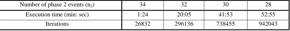
Shih and Revelle used an IBM 3090-600J super computer to run their model. As mentioned earlier, even using these revisions, it was not possible to reach a solution in lower values of n2 by a Pentium II computer. Therefore, further improvements were required before the model could be practically applied using the publicly available computers. Assuming α1 = 0.75 and α2 = 0.60 for the example in Shih and Revelle [6], the model was executed using different phase 2 frequencies. It was noticed that as n2 is reduced, the computer execution time is exponentially increased (Table 1).

Further investigation of the solutions revealed that some of the results stay the same from one n2 level to another. In fact, as Table 2 shows solutions TABLE 1. Computer Execution Time Required for Different N2’s – Method 1.

Number of phase 2 events (n2) 34 32 30 28

Execution time (min: sec)

1:24 20:05 41:53 52:55

Iterations

of Y2 that are equal to 1 stay the same with reduced n2 levels. This is obvious, since as the frequency of phase 2 hedging is reduced, number of phase 1 hedging events must increase. If we call

∆n to be the difference between the two subsequent assumed n2 levels, then as n2 is reduced ∆n periods must take either a phase 1 or full demand commitment level. In either case, they will have Y2 equal to 1. In this process, ∆n periods of phase 2 must be raised to phase 1 level. To do this some of the full commitment levels must be changed to phase 1, so that the extra water gained from this transaction could be used to rise ∆n periods from phase 2 to phase 1. Therefore, reducing n2 will usually increase frequency of phase 1 (cases with Y2 = 1 and Y1 = 0) and decrease frequency of full success (cases with Y1 = 1 and Y2 = 1).

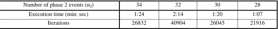
To further reduce the computer execution time and memory, we used the above-mentioned results. Starting from a high n2 level, such as 34 in this case, we may easily reach a solution. In the next step, we set n2 equal to a lower value such as 32, and transfer those results of Y2 from the previous step that were found to be 1. Computer execution time of this method will be much less than the earlier method. By continuing this procedure, we

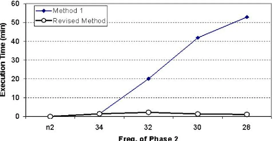
would easily solve the model for values of n2 as small as 10. It is possible to apply this technique for solutions of more sophisticated models within acceptable time and memory spans. It is also practically possible to further increase the number of hedging phases. Table 3 show the execution time and iterations required for the same problem when the new procedure is applied. Figure 2 clearly shows the superiority of the proposed method.

In Figure 3 results of Shih and Revelle [6] and the proposed method are compared. It is noticed that in overall the proposed method has higher frequencies of full demand commitments. This is clearly true for lower levels of n2, where proper allocation of available water is crucial.

3. CASE STUDY

The revised method is applied to Karadj reservoir located in northwest of Tehran. The reservoir is the major source of municipal water supply for Tehran, the capital. It is also used to provide irrigation water needs of downstream valley. Table 4 shows Tehran’s mean monthly water demand from Karadj reservoir. Note that orders of the months are based on typical Iranian water year. It starts on the first day of each fall and ends on the last day of each summer.

In our study, we used 40 years of monthly historical inflow as well as 20 series of synthetically generated data of the same length. For this purpose, a single and a multi-variate AR model were used to generate 10 series of reservoir inflow each. Table 5 shows a summary of long-term parameters of historical and generated data.

The model was prepared and the proposed method was applied using α1 = 0.75 and α2 = 0.60. For this purpose, droughts with three, two, and one-year long durations were identified from the historical data and used to develop the hedging rules. Frequency of different hedging levels for a TABLE 2. Changes in the Solution of Y2 with Different N2

Levels.

n2 = 34 n2 = 32 n2 = 30 n2 = 28

Y2( 3, 4) 0 0 0 0

Y2( 3, 5) 0 0 0 1

Y2( 3, 6) 0 0 0 1

Y2( 3, 7) 0 0 1 1

Y2( 3, 8) 0 0 1 1

Y2( 3, 9) 0 1 1 1

Y2( 3, 10) 0 1 1 1

Y2( 3, 11) 1 1 1 1

Y2( 3, 12) 1 1 1 1

TABLE 3. Computer Execution Time Required for Different N2 Levels Using the Proposed Method.

Number of phase 2 events (n2) 34 32 30 28

Execution time (min: sec)

1:24 2:14 1:20 1:07

Iterations

three-year drought is illustrated in Figure 4. Similar charts were depicted for two and one-year droughts. In Figure 5 rule curves analogous to the well-known form of reservoir rule curves are shown. These curves are simply derived from the hedging threshold levels.

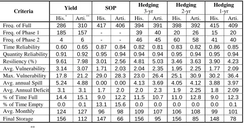
In the next step, suitability of the hedging rules was investigated through simulation of the system by historical and synthetic data. Meanwhile, a

yield model and standard operating procedure (SOP) were also used for comparison purposes. Table 6 shows the summary of the results. It should be noted that the values shown under the artificial columns are the average of all series. The yield model (YM) is developed using firm and secondary yields equal to 60 and 15 percent of total demand. The initial storage for all models is assumed to be 100 mcm. It is noticed that YM is Figure 2. Comparison of execution time of the methods.

not successful in making full demand commitments and its resiliency is high, however its maximum vulnerability is much less than any other rule. On the other hand, SOP has the highest

frequency of full success, but it also exerts the highest maximum vulnerability among the others with the exception of 1-year hedging rule. In fact, the SOP and 1-year hedging rules behave similar in TABLE 4. Monthly Municipal Water Demand of Tehran from Karadj Reservoir (mcm).

month 1 2 3 4 5 6 7 8 9 10 11 12

demand 34.4 30.2 25.4 25.1 23.3 24.2 26.8 46.8 57.6 52.8 45.7 41.3

TABLE 5. Monthly Parameters of Historical and Generated Reservoir Inflow.

Data Type Parameter 1 2 3 4 5 6 7 8 9 10 11 12

Avg. (mcm) 15.1 17.3 15.5 13.8 14.7 26.5 61.8 102.3 87.0 50.3 26.6 17.6

Stdev. 3.4 8.1 8.2 4.8 4.1 13.5 23.2 33.5 31.8 20.7 9.3 4.9

Historical

_{r 0.70 0.79 0.76 0.68 0.33 0.68 0.73 0.82 0.96 0.96 0.94 0.66}

Avg. (mcm) 26.4 21.9 18.1 15.9 14.8 23.4 50.9 80.9 80.2 50.2 40.2 34.1

Stdev. 6.3 6.5 6.5 6.5 5.7 29.5 57.2 34.3 28.1 15.3 9.8 8.1

Generated ARMV

_{r 0.99 0.98 1.00 0.97 0.26 0.23 0.53 0.96 0.98 0.96 0.98 0.46}

Avg. (mcm) 15.0 17.0 15.6 14.0 15.0 26.2 62.7 101.5 87.4 50.2 26.5 17.5

Stdev. 3.2 6.2 5.9 4.1 4.1 10.5 25.5 34.4 32.3 19.7 8.8 4.4

Generated AR

r 0.73 0.80 0.87 0.70 0.51 0.55 0.73 0.82 0.96 0.96 0.94 0.73

0 5 1 0 1 5 2 0 2 5 3 0 3 5 4 0

1 6 1 8 2 0 2 2 2 4 2 6 2 8 3 0 3 2 34

n2

Mo

n

th

s

w ith o u t ra ti o ni n g p h a se 1 p h a se 2

most aspects. SOP also faces more empty reservoir storages than any other model.

Although the 3-year hedging rule indicates slightly lower frequencies of full success, however Figure 5. Hedging rule curves for Karadj reservoir.

TABLE 6. Summary of Results.

Yield SOP Hedging

3-yr

Hedging 2-yr

Hedging 1-yr Criteria

His.* Arti.** His. Arti. His. Arti. His. Arti. His. Arti.

Freq. of Full 286 310 417 406 394 391 398 392 415 409

Freq. of Phase 1 185 157 - - 39 40 20 26 15 20

Freq. of Phase 2 4 6 - - 46 45 60 58 41 40

Time Reliability 0.60 0.65 0.87 0.84 0.82 0.81 0.83 0.82 0.86 0.85

Quantity Reliability 0.91 0.92 0.95 0.94 0.94 0.94 0.95 0.94 0.95 0.94

Resiliency (%) 9.61 7.98 3.01 2.56 4.81 5.03 3.46 3.63 3.90 4.23

Avg. Vulnerability 3.14 3.07 1.71 2.03 2.04 2.35 1.95 2.25 1.77 2.09

Max. Vulnerability 17.8 21.2 29.0 28.3 23.0 26.4 25.1 30.9 30.2 36.4

Avg. annual Spill 5.24 4.88 0.00 0.00 4.13 3.69 4.05 4.12 3.88 3.97

Avg. Annual Deficit 3.1 3.1 1.7 2.0 2.0 2.3 1.9 2.25 1.8 2.09

% of Time Full 14.4 15.1 9.0 12.2 11.5 10.7 11.0 12.8 9.0 12.3

% of Time Empty 0.0 0.1 13.1 15.6 0.0 0.0 0.0 0.0 0.0 0.1

Avg. Monthly 124 127 96 98 109 107 106 108 99 101

Final Storage 156 112 147 66 156 95 156 85 148 78

*

historical data. **

its maximum vulnerability is much less than SOP. The results also indicate that as we shift from 3-year to 1-3-year modeling of droughts we slightly gain more frequency of success, however the systems maximum vulnerability rises greatly. Although not presented in here, both models of synthetic data generation show similar results. The values indicated in the Table are the average of all 20 series.

4. CONCLUSIONS

The hedging model as developed by Shih and Revelle [6] is not suitable for practical applications. It requires supercomputers to run. A simple method is developed that greatly reduces computer execution time and memory requirements. The proposed method allows the model application with the publicly available computers. It also makes further increase in the number of hedging levels or extension of time horizon practically possible. It was also compared with the original model based on the example from Shih and Revelle [6]. The results indicated higher frequencies of full success by the new method.

To further illustrate the method, it was applied to the Karadj reservoir system in Iran. The results show that a 3-year hedging rule has slightly lower

frequency of full release commitment, however its maximum vulnerability is much less than SOP. When compared to the yield model, its reliability is much higher. The yield model has the lowest maximum vulnerability among all of the models experienced in this paper.

5. REFERENCES

1. Shih, J. S. and Revelle, C., “Water Supply Operation

During Drought: Continuous Hedging Rule”, J. of Water

Reso. Plann. and Manag., 120(5), (1994), 613-629. 2. Dariane, A. B., “Optimization of Reservoir Operation

During Droughts by Hedging Rule”, Hydrology Days,

Proceedings of the Nineteenth Annual American Geophysical Union, August 16-20, Colorado State University, Fort Collins, (1999), 84-96.

3. Bayazit, M. and Unal, E., “Effect of Hedging on Reservoir

Performance”, Water Reso. Res., 26(4), (1990), 713-719.

4. Srinvasan, K. and Philipose, M. C., “Evaluation and Selection of Hedging Policies Using Stochastic Reservoir

Simulation”, Water Reso. Manag., 10(3), (1996), 163-188.

5. Srinvasan, K. and Philipose, M. C., “Effect of Hedging on

Over-Year Reservoir Performance”, Water Reso. Manag.,

12(2), (1998), 95-120.

6. Shih, J. S. and Revelle, C., “Water Supply Operation

During Drought: A Discrete Hedging Rule”, European J.

of Oper. Res., Vol. 82, (1995), 163-175.

7. Neelakantan, T. R. and Pundarikanthan, N. V., “Hedging Rule Optimization for Water Supply Reservoir System”,