Subspace system identification

Subspace system identification

J. Poshtan and H. Mojallali

Abstract: We give a general overview of the state-of-the-art in subspace system identification methods. We have restricted ourselves to the most important ideas and developments since the methods appeared in the late eighties. First, the basis of linear subspace identification are summarized. Different algorithms one finds in literature (Such as N4SID, MOESP, CVA) are discussed and put into a unifying framework. Further, a comparison between subspace identification and prediction error methods is made on the basis of computational complexity and precision of methods by applying them to a glass tube manufacturing process.

Keywords: subspace methods, system identification, state-space methods, multivariable systems, linear algebra.

1 Introduction1

Mathematical models of dynamical systems are used for analysis, simulation, prediction, optimization, monitoring, fault detection, training and control. There are several approaches to generate a model of a system. One could for instance start from first principles, such as writing down basic physical or chemical laws that generate behavior of the system. This so called white box approach works for simple examples, but its complexity increases rapidly for real-world systems. In some cases, equations of the system are known up to within some unknown parameters, which are estimated using some parameter-estimation method (gray box modelling). Both, two aforementioned techniques require the extraction of system equations which is difficult in MIMO systems due to system variables interaction and often leads to several trial and error stages. Another approach is provided by system identification, in which measurements or observations are first collected from the system, and then modeled using a so called black-box identification approach. Such an approach basically consists of first defining a parameterization of the model, and then determining the model parameters in such a way that the measurements are explained as accurately as possible by the model. In system identification, parameterization and model selection are important. [1], [2], [9], [10], [11] represent some techniques for model parameterization. [8] represents a kind of parameterization called observability model, in which the user should ultimately select a desired model from model sets. All of proposed techniques, with their advantages and disadvantages, for starting require prior knowledge such as system order. Therefor, usage of the these techniques take a lot of time and operations and several trial and error stages must be done. The beginning of the 1990s witnessed the birth of a new type of linear system identification algorithms, called subspace methods. Subspace methods basically originate in a good combination between system theory, geometry and numerical linear algebra. It is shown that subspace methods calculate a good state

Iranian Journal of Electrical & Electronic Engineering, 2005. Paper first received 27th May 2002 and in revised from 3th February 2004.

J. Poshtan and H. Mojallali are with the Department of Electrical Engineering, Iran University of Science and Technology, Narmak, Tehran 16844, Iran.

space model without any priori knowledge of the system. This paper consists of the following sections: First of all, we briefly review the main concepts and algorithms of linear subspace system identification(section2). Different methods found in literature are presented and put into a unifying framework. Further we comment on the comparison between prediction error methods and subspace identification methods by applying them to a glass tube manufacturing process.

2 An overview of the theory[6]

Models and/or systems can be roughly divided into classes, such as linear and nonlinear, time-invariant or time-varying, discrete-time or continuous-time, with lumped or with distributed parameters, etc. While at first sight, the class of linear time-invariant models with lumped parameters seems to be rather restricted, it turns out in practice that many real-life input-output behaviors of practical, industrial processes can be approximated very well by such models. Linear subspace identification methods are connected with systems and models of the form:

k k k 1

k Ax Bu w

x + = + + (1)

k k k

k Cx Du v

y = + + (2)

with

(

)

0

R S

S Q v w v w

E T pq

t q t q p

p

³ d ÷÷ ø ö çç è æ = ú ú û ù ê

ê ë é

÷ ÷ ø ö ç ç è æ

(3)

The vectors m1 k R

u Î ´ and l1

k R

y Î ´ are the measurements at time instant k of respectively the

minputs and loutputs of the process. The vector xkis

the state vector of the process at discrete time instant k, 1

l k R

v Î ´ and n1

k R

w Î ´ are unobserved vector signals, called the measurement noise and the process noise, respectively. It is assumed that they are zero mean, stationary white noise vector sequences and uncorrelated with the inputs uk. AÎRn´nis the system matrix, _BÎRn´m_{is the input matrix, CÎR}l´n_{is the} output matrix while _DÎRl´m _{is the direct feed-through} matrix. The matrices _QÎRn´n_{, SÎR}n´l_{and RÎR}l´l_are

the covariance matrices of the noise sequences wkand

k

v . In subspace identification, it is typically assumed that the number of available data points goes to infinity,

and that the data is ergodic. We are now ready to state the main problem treated:

Given a number of measurements of the input ukand the output ykgenerated by the unknown system (1)-(3);

Determine the order n of the unknown system, the system matrices A,B,C, D up to within a similarity transformation, and the matrices Q, S, R.

In this section, we will first describe the general concepts in subspace identification . Further, the two basic steps all subspace methods consist of are presented. Finally, the different algorithms existing in the literature are analyzed in a unifying framework. Subspace identification algorithms always consist of two steps. The first step makes a projection of certain subspaces generated from the data, to find an estimate of the extended observability matrix and/or an estimate of the states of the unknown system. The second step then retrieves the system matrices from either this extended observability matrix or the estimated states. We will come back to this in section 2.2.2, where we describe different subspace identification methods and fit them into a unifying framework.

2.1 The subspace structure of linear systems

The following input-output matrix equation[4], played a very important role in the development of subspace identification: f f s i f d i i i

f X H U H M N

Y =G + + + (4)

The different terms in this equation are now defined: The extended observability matrixGi is defined as:

÷÷ ÷ ÷ ÷ ÷ ÷ ø ö çç ç ç ç ç ç è æ = G -1 i 2 i CA CA CA C  (5)

The deterministic lower block triangular Teoplitz matrix d

i

H is defined as:

÷÷ ÷ ÷ ÷ ÷ ÷ ø ö çç ç ç ç ç ç è æ =

-- _{B CA B CA B D}

CA 0 D CB CAB 0 0 D CB 0 0 0 D H 4 i 3 i 2 i d i          (6)

The stochastic lower block triangular Teoplitz matrix s

i

H is defined as:

÷÷ ÷ ÷ ÷ ÷ ÷ ø ö çç ç ç ç ç ç è æ =

-- _{CA CA 0}

CA 0 0 C CA 0 0 0 C 0 0 0 0 H 4 i 3 i 2 i s i         (7)

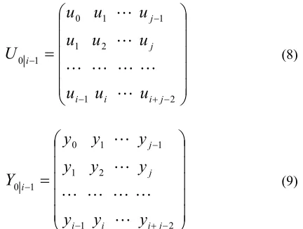
The input and output block Hankel matrices are defined as:

÷

÷

÷

÷

÷

ø

ö

ç

ç

ç

ç

ç

è

æ

=

-+ -2 1 2 1 1 1 0 1 0 j i i i j j i

u

u

u

u

u

u

u

u

u

U















(8)

÷

÷

÷

÷

÷

ø

ö

ç

ç

ç

ç

ç

è

æ

=

-+ -2 1 2 1 1 1 0 1 0 j i i i j j i

y

y

y

y

y

y

y

y

y

Y















(9)

where we assume that j®¥throughout the paper. For convenience and short hand notation, we call:

1 i 2 i f 1 i 0 p 1 i 2 i f 1 i 0 p Y Y , Y Y U U , U U -= = = =

where the subscript pand f denote respectively the past and the future. The matrix containing the inputs

p

U and outputs Ypwill be called Wp:

÷ ÷ ø ö ç ç è æ = p p p _U Y W

The block Hankel matrix formed with the process noise k

w and the measurement noise vkare defined respectively as M_0i-1 and N_0i-1 in the same way. Once again, we define for short hand notation:

1 i 2 i f 1 i 0 p 1 i 2 i f 1 i 0 p N N , N N M M , M M -= = = =

We finally denote the state sequence Xias:

) x x x x (

Xi= i i+1 i+2  i+j-1 (10) Definition(Orthogonal projection)

The orthogonal projection of the row space of A into the row space of B is denoted by AB and defined as:

B AB B

A ₌ +

^

B

A is the projection of the row space of

A

into

B

^, the orthogonal complement of the row space of

B

, for which we have

B A A B

A _{^ =}

-2.2 The two basic steps in subspace identification

In this section we will explore the two main steps that all subspace algorithms consist of (see Figure 1). The first step always performs a weighted projection of the row space of the previously defined data Hankel matrices. From this projection, the observability matrix

i

G and/or an estimate Xi

~

of the state sequence Xican

be retrieved. In the second step, the system matrices A,

B, C, D and Q, S, Rare determined. As shown in Figure 1, a clear distinction can be made between the algorithms that use the extended observability matrix

i

Gto obtain the state space matrices, and those using the estimated state sequence Xi

~

.

Fig. 1 Two main steps in subspace algorithms.

First step: finding the state sequence and/or the extended observability matrix

In this section, we show how an orthogonal projection with data block Hankel matrices forms one of the key elements in subspace system identification algorithms. All subspace methods start from the previously presented matrix input-output equation (4), from which it can be observed that the block Hankel matrix containing the future outputs Yfis related in a linear way to the future input block Hankel matrix Uf and the future state sequence Xi. The basic idea of subspace identification now is to try to recover the GiXi-term of this equation. This is a particularly interesting term since either the knowledge of Gi or Xi leads to the system parameters (see next section). Moreover, GiXiis a rank-deficient term(of rank n, i.e. the system order!) which means that once GiXiis known, Giand Xi can be simply found from a SVD.

How can an estimate of GiXibe extracted from the above equation? For this we need the previously defined notion of orthogonal projection. By projecting the row space of Yfinto the orthogonal complement U^f of the row space of Ufwe find:

^ ^ ^

^=G + +

f f f f s i f i i f f

U N U M H U X U Y

Since it is assumed that the noise is uncorrelated with the inputs, we have that:

f f f f

f

f _N

U N , M U

M _{= =}

^ ^

Therefore:

f f s i f i i f

f _{HM N}

U X U

Y ₌G _{+ +}

^ ^

The following step consists in weighting this projection to the left and the right with some matrices W1and W2:

2 f f s i 1 2 f i i 1 2 f f

1.Y _U .W W. X _U .W W.(HM N ).W

W ^ = G ^ + +

Of course, the inputs Ufand the weighting matrices 1

Wand W2cannot be chosen arbitrarily but they should satisfy the following 3 conditions:

1. rank(W1.Gi)=rankGi (11)

2. .W)

U X ( rank X

rank 2

f i

i= ^ (12)

3. W1.(HsiMf+Nf).W2=0 (13)

The first two conditions guarantee that the

rank-nproperty of GiXiis preserved after projection onto

^

f

U and weighting by W1and W2. The third condition expresses that W2 should be uncorrelated with the noise sequences wkand vk.

If these three conditions are satisfied, we have that:

2 f i i 1 2 f f 1

i W.Y _U .W W. X _U .W

O = _^ = G _{^ (14)}

with SVD:

(

)

_÷÷

ø ö ç ç è æ ÷÷ ø ö çç è æ

= _T

2 T 1 1

2 1 i

V V 0 0

0 S U U O

The following important properties can now be stated:

T 2 2 / 1 2 f i

2 / 1 1 1 i 1

i

V S W . U X

S U . W

n O rank

= = G

=

^

Obviously, the singular value decomposition of the matrix Oi delivers the order nof the system. Moreover, from the left singular vectors corresponding to non-zero singular values, the extended observability matrix Gican be found (up to a similarity transformation), whereas the right singular vectors contain information about the states Xi. If the weighting matrix W2is such that it has

jcoloumns, the matrix

2 f i i X _U .W

X~ = _{^ (15)}

can indeed be considered as an estimate of the state sequence

X

_i. It was shown [11] that, for a particular choice of W2, Xi

~

is a kalman filter estimate of Xi. One might wonder about the effect of choosing the weights

1

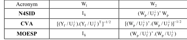
Wand W2 in (14). Without going into details here, it suffices to say that, by choosing appropriate weighting matrices W1and W2, all subspace algorithms for LTI systems can be interpreted in the above framework, including N4SID, MOESP and CVA (see Table 1). At this point, a clear distinction can be made between the algorithms that start from Gito find the system matrices

A,B,C,D(MOESP) and those that use i

X~ (N4SID,CVA).

Second step: finding the state space model We have found how an estimate Xi

~

of the state sequence Xiand the extended observability matrix

i

Gcan be retrieved from the weighted projection (14) of the future outputs Yfinto the orthogonal complement of future inputs Uf. In what follows, we discuss the two classes of subspace identification algorithms mentioned above. The first class uses the state estimates

X

~

_i(the right singular vectors) to find the state space model. Algorithms that follow this approach are N4SID and CVA. The second class of algorithms uses the extended observability matrix Gi(i.e. the left singular vectors) to find the model parameters.

i G

Input-output data u_k, y_k

i

X~

System matrices

R , S , Q , D , C , B , A

STEP 1

STEP 2

Table 1 This table interprets different existing subspace identification algorithms in a unifying framework

Acronym W1 W2

N4SID Ili (Wp/Uf^)+Wp

CVA T 1/2

f f f

f/U ).(Y /U ) ]

Y

[( ^ ^ - 1/2

f p f

p/U ) .(W /U )]

W

[( ^ + ^

-MOESP Ili (Wp/Uf^)+.(Wp/Uf^)

Algorithms using an estimate Xi

~

of the state sequene The estimated state sequence Xi

~ _{can be interpreted as}

the solution of a bank of Kalman filters, working in parallel on each of the columns of the matrix Wp. Besides Xi

~ _{, we also need the state sequence}

1 i

X~+ . This

sequence can be obtained from a Oi+1 projection and weights W1, W2 in (14) based on W0i, Yi+12i-1and

1 i 2 1 i

U_{+ -}(see section 2.1 for notations). This leads to the sequence Oi+1and the Kalman filter states Xi1

~ + : 2 1 i 1 i 1 2 1 i 2 1 i 1 i 2 1 i 1 1

i X .W

~ . W W . U Y . W

O ^ - +

-+ -+

+ = = G

System model: The state space matrices A,B,Cand

Dcan now be found by solving a simple set of over-determined equations in a least-squares sense:

÷÷ ø ö çç è æ r r + ÷ ÷ ø ö ç ç è æ ÷÷ ø ö çç è æ = ÷ ÷ ø ö ç ç è æ ₊ v w i i i i i 1 i U X~ D C B A Y X~ (16)

with obvious definitions for rwand rvas residual matrices. This reduces to

2 F i i i i i 1 i D , C , B , A U X~ D C B A Y X~

min _÷÷

ø ö ç ç è æ ÷÷ ø ö çç è æ -÷ ÷ ø ö ç ç è æ ₊

Noise model: The noise covariance Q,Sand Rcan be estimated from the residuals rwand rvas:

(

)

0

. j 1 R S S Q _T v T w v w i T ³ ú ú û ù ê ê ë é r r ÷÷ ø ö çç è æ r r = ÷ ÷ ø ö ç ç è æ

where the index i denotes a bias induced for finite i, which disapears as i®¥. As is obvious by construction , this matrix is guaranteed to be positive semi-definite. This is an important feature since only positive definite covariances can lead to a physically realizable noise model.

Algorithms using the extended observability matrix i

G

contrary to the previous class of algorithms, here the system matrices are determined in two separate steps: first, Aand Care determined from Giwhile in a second step Band Dare computed.

Determination of A and C

The matrices A and C can be determined from the extended observability matrix in different ways. All the methods, make use of the shift invariance property of the matrix Gi, which implies that (Kung,1978)( following Matlab notations):

( )

1: ,l:

C ,

.

A=G_i+G_i =G_i

Determination of B and D

After the determination of Aand C, the system matrices B and D have to be computed. Here we will

only sketch one possible way to do so. From the input-output equation (4), we find that:

_(lin)li _limi

mi ) n li ( _R d i R i R f f

i YU . H

´ ´ -´

- _{Î Î}

^ Î

+

^ _{= G}

G_



where (li n) li i^ÎR - ´

G is a full row rank matrix satisfying

0 . _i

i G =

G^ _{. Here once again the noise is cancelled out}

due to the assumption that the input ukis correlated with the noise. Observe that with known matrices

A,C,_G^

i , Ufand Yf, this equation is linear in Band

D.

3 An industrial glass tube manufacturing process identification

3.1 Process description [4]

The outline of the process is shown in Figure 2. By indirect electric heating the glass is melted and it flows down through a ring shaped hole along a mandrill. Shaping of the tube takes place at, and just below the end of the mandrill. The glass tube is pulled down due to gravity and a drawing machine. Two measures of dimention, wall thickness and diameter of the tube, are the most important quantities to be regulated (and thus to be identified), hence they are the outputs of the process. The mandrill gas pressure and the drawing speed can affect the wall thickness and the diameter most directly and easily, so they are good candidates for inputs. Other variables such as the power supplied to melt the glass, the pressure in the melting vessel and the room temperature will be considered as disturbances. Therefore the process can be modeled as a input 2-output process with disturbances (combined deterministic-stochastic model). For the purpose of identification, the process was excited with an orthogonal white PRBN sequence. The two inputs and outputs were recorded. The diameter is measured in two orthogonal directions and averaged out. The wall thickness is measured in four directions in a plane, and once again, these measurements are averaged out. The input and output signals are scaled so that the original signals can not be retrieved. The input and output signals are made zero mean, filtered with a third order low pass butterworth filter with a cutoff frequency equal to (f_s/2)/10 wherefsis the sampling frequency. The outputs are then detrended, as typically the thickness has a trend in it. Then the delays between the inputs and outputs are determined through a simple correlation analysis. The signals are corrected for these delays. The first 500 samples are neglected (transiant effects).

3.2. Subspace Identification vs. Prediction Error Method

In this section, we will compare the identification results obtained using the three subspace algorithms with the results from the classical identification techniqe (PEM). We used signals of 1326 samples from this system , The first 900 samples for identification and the remaining 426 samples for validation. The results are summarized in table 2. For subspace algorithms, the

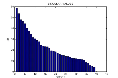
order can be determined through the inspection of a singular value plot (Figure 3). In noise-free case, the model order is equal to the number of nonzero singular values [4]. In a noisy case such as our process, however, the model order was chosen to be equal to 8 resulting the least prediction error. Among the three subspace algorithms, CVA led to the least prediction error for this case study. For using PEM classical identification, an initial model is required. Therefore, for this purpose PEM was initialized with the model from N4SID algorithm. Input signals used for identification are shown in Figure 4. In this Figure, measured and predicted output signals for CVA model are shown. It should be noted that for the prediction of the output signal, a Kalman fiter was used for the following model:

k k k k

k k k 1 k

e Du Cx y

Ke Bu Ax x

+ + =

+ + =

+

Meanwhile, the error related to a deterministic prediction is shown in table 2.

Fig. 2 The glass tube production process

Fig. 3 Singular values as a function of the model order. The

model order is chosen to be 8.

4 Conclusion

In this paper, we have given a brief overview of the linear subspace system identification methods. We made a clear distinction between methods using the states and methods statrting from the observability matrix to recover the system parameters. Further, a direct comparison was made between subspace algorithms and PEM identification method on the basis of accuracy and computation time. Therefore, all methods were applied to a real-life process. The conclusion is that subspace methods calculate a state space model without a-priori fixed parametrization, and this is a fast and numerically reliable way. Subspace methods and prediction error methods are complementary in the sense that a good initial model can be quickly obtained with subspace methods while a further optimization of parameters (if possible) can be done with prediction error methods.

Table 2 Comparison of three subspace algorithm and PEM classical identification. The second row indicates the chosen order. The

third row indicates the number of block rows that is used in the past and future block Hankel matrices of subspace algorithms. The fourth row indicates number of iterations related to each algorithm. The fifth row shows the number of floating point operations. The sixth shows consuming time for these algorithms in second. The seventh row is the errors (in percent) between the measured validation outputs and the simulated outputs using only the deterministic subsystem. The eighth row shows the error between measured and kalman filter one step ahead prediction. With [yvk]ithe

i

th validation output channel and [ysk]ithe

i

th simulated

output channel, total error is defined as (Nv=426): %

) ] y ([

) ] y [ ] y ([ 100

v v

N

1 k

2 i v k N

1 k

2 i s k i v k

å

å

= =

-=

e

algorithm N4SID MOESP CVA PEM

order 8 8 8 8

Number of block rows 20 20 20 20

iterations - - - 10

flops 61980981 81280318 63415534 314708169

time 4 5 4 25

Prediction error(deterministic) 30.8 29.1 43.7 34.4

Prediction error(Kalman filter) 14 13.5 13 14

0 5 10 15 20 25 30 35 40 45 0

10 20 30 40 50 60

dB

SINGULAR VALUES

ORDER

Fig. 4 Input and output signals used for identification. The inputs are drawing speed and mandrill pressure. The outputs are diameter and thickness. The dotted lines shows one step ahead predicted outputs from CVA model. Prediction errors have shown in figure.

5 References

[1] C.T. Chou, Geometry of linear systems and identification, PHD Thesis, Trinity college, Cambridge, England ( March 1994).

[2] C.T. Chou and J.M. Maciejowsky , System identification using balanced parametrizations, IEEE Trans. On Automatic Control, 42 (7) 956-974 (1997).

[3] P.T. Kabamba, Balanced forms: Canonicity and parametrization, IEEE Trans. On Automatic Control, 30(11) 1106-1109 (1985).

[4] B. DeMoor, P. DeGersem, B. Deschutter, W. Favoreel, DAISY: A database for identification of systems, Journal A, Special Issue on CACSD (Computer Aided Control Systems Design), 38 (3) 4-5 (1997).

0 50 100 150 200 250 300 350 400

-2 -1 0 1 2 3

D

ra

w

in

g

S

pe

ed

0 50 100 150 200 250 300 350 400

-3 -2 -1 0 1 2

M

an

dr

el

l P

re

ss

ur

e

0 50 100 150 200 250 300 350 400 450

-4 -2 0 2 4

D

ia

m

et

er

0 50 100 150 200 250 300 350 400 450

-4 -2 0 2 4

Th

ic

kn

es

s

Error

Error

[5] B. DeMoor, Mathematical concepts and techniques for modeling of static and dynamic systems, PHD Thesis, Department of Electrical Engineering, Katholike Universiteit Leuven, Belgium(1988). [6] W. Favoreel, B. DeMoor and P. Vanoverschee,

Subspace state space system identification for industrial processes, Journal of Process Control, 10 140-155 (2000).

[7] W.E. Larimore , Canonical variate analysis in identification, filtering and adaptive control, in proc. 29th _{Conference on Decision and Control,} Hawai, 596-604 (1983).

[8] L. Ljung , System Identification-Theory for the User, Prentice Hall , Englewood cliffs, N.J (1999).

[9] T. Mckelvey, Identification of state space models from time and frequency data, PHD Thesis, No. 380, Departmet of Electrical Engineering, Linkoping, Sweden (1995).

[10] B.C. Moore, Principal component analysis in linear systems: Controllability, observability and model reduction, IEEE Trans. On Automatic Control, 26(1) 17-32 (1981).

[11] P. Vanoverschee and B. DeMoor, N4SID: subspace algorithms for the identification of combined deterministic and stochastic systems, Automatica, 30(1) 75-93 (1994).

[12] M. Verhaegen and P. Dewilde , Subspace identification, part I: the output-error state space model identification class of algorithms, Int. J. Control , 56 1187-1210, (1992).