A NEW TECHNIQUE FOR THE CALCULATION
OF COLLIDING VORTEX RINGS
T.K. Sheel
Department of Mathematics, Shahjalal University of Science and Technology Sylhet 3114, Bangladesh
[email protected] - [email protected]
(Received: May 29, 2008 – Accepted in Revised Form: September 25, 2008)
Abstract The present study involves a novel computational technique, regarding simultaneous use
of the pseudo particle method, Poisson integral method and a special-purpose computer originally designed for molecular dynamics simulations (MDGRAPE-3). In the present calculations, the dynamics of two colliding vortex rings have been studied using the vortex method. The present acceleration technique allows the calculation of 107 vortex elements. The reconnection of the vortex
rings was clearly observed, and the discretization error was nearly negligible.
Keywords Vortex Method, Vortex Ring, Special-Purpose Computer, Fast Multipole Method
ﻩﺪﻴﻜﭼ
ﻪﻟﺎﻘﻣﺮﺑﻞﻤﺘﺸﻣﺮﺿﺎﺣ ﮏﻳ
ﺵﻭﺭ ﺪﻳﺪﺟﻲﺗﺎﺒﺳﺎﺤﻣ ﺓﺭﺎﺑﺭﺩﻪﮐﺖﺳﺍ
ﺩﺎﻔﺘﺳﺍ ﺓ ﺵﻭﺭﺯﺍﻥﺎﻣﺰﻤﻫ ﻩﺭﺫﻪﺒﺷ
،
ﺵﻭﺭ ﻦﺳﺁﻮﭘ ﻊﻤﺠﺗ ﮏﻳ ﻭ
ﺩﺮﺑﺭﺎﮐ ﺎﺑ ﻪﻧﺎﻳﺍﺭ ﺹﺎﺧ
ﻝﻮﮑﻟﻮﻣ ﮏﻴﻣﺎﻨﻳﺩ ﻱﺯﺎﺳ ﻪﻴﺒﺷ ﻱﺍﺮﺑ ﻞﺻﺍ ﺭﺩ ﻪﮐ ﺎﻫ
(MDGRAPE-3)
ﺩﻮﺑ ﻩﺪﺷ ﻲﺣﺍﺮﻃ ﻩ
ﻲﻣ ﺩﺯﺍﺩﺮﭘ
.
ﺕﺎﺒﺳﺎﺤﻣ ﺭﺩ ﺮﺿﺎﺣ
ﻘﻠﺣﻭﺩ ﮏﻴﻣﺎﻨﻳﺩ ، ﺔ
vortex
ﻢﻫ ﺭﺩ ﺎﺑﻩﺪﻧﻭﺭ
ﺵﻭﺭ ﺯﺍﻩﺩﺎﻔﺘﺳﺍ
vortex
ﺖﺳﺍ ﻩﺪﺷﻲﺳﺭﺮﺑ
.
ﺏﺎﺘﺷﺵﻭﺭ ﺪﻨﻫﺩ
ﺓ ﻪﺋﺍﺭﺍ ﺯﺎﺟﺍﻩﺪﺷ ﺓ ﺕﺎﺒﺳﺎﺤﻣ ۱۰۷
ﻥﺎﻤﻟﺍ
vortex
ﺍﺭ
ﻲﻣ ﺪﻫﺩ
.
ﺭﺎﺑﻭﺩ ﻁﺎﺒﺗﺭﺍ ﻭ ﺩﺭﻮﺧﺮﺑ ﺓ
ﻪﻘﻠﺣ ﯼﺎﻫ
vortex
ﻪﺑ ﺑﻮﺧ ﯽ ﺯﺍ ﻲﺷﺎﻧ ﻱﺎﻄﺧ ﻦﻴﻨﭽﻤﻫ ﻭ ﺖﺳﺍ ﻩﺪﺷﺺﺨﺸﻣ
ﻲﻄﺧ ﻥﺩﺮﮐ ، ﺰﻴﭼﺎﻧﺭﺎﻴﺴﺑ ﺖﺳﺍ
.
1. INTRODUCTION
Fast N-body solvers are essential to the vortex method calculation of turbulent flows. A direct calculation of the mutual interaction of N particles is proportional to N2. Due to this enormous calculation cost, the original purpose of vortex methods was not to perform a direct numerical simulation of the flow, but to somewhat mimic the dominant vortex dynamics using discrete vortex elements.
The use of fast algorithms made it possible to achieve a scaling of O(N) [1], and these algorithms have been successfully applied to vortex methods [2-4]. Furthermore, accurate viscous diffusion schemes were introduced, which enabled vortex methods to tackle flows with high viscosity accurately [5]. The combination of these two innovations led to a new paradigm, i.e. solving flows of moderate Reynolds numbers and fully resolving these flows. The vortex method was recognized as a discretization method rather than an attempt to model vortex dynamics, because the computational power that was necessary to prove
these claims became available.
However, the high proportionality constant of the fast N-body solvers prevented them from matching the speed of grid based fast Poisson solvers. Since the mainstream methods in computational fluid dynamics use grid based fast Poisson solvers, it was still difficult for vortex methods to be considered as an alternative to conventional grid based methods.
Another way to fill the gap between the N-body solver and fast Poisson solver is to use a hardware specialized for N-body calculations, such as the MDGRAPE-3 [8]. Ever since the GRAPE [9] was first introduced, these special purpose computers have constantly outperformed the general-purpose computers of the same price [8]. At this point, it is not yet evident which will prevail: Grid based fast Poisson solvers on parallel general purpose architecture, or fast N-body solvers on parallel special purpose processors. In my previous study, I have calculated the direct part of the FMM on the MDGRAPE-3 [10]. In the present study, the possibility of calculating the entire fast multipole method (FMM) on the MDGRAPE-3 will be investigate by using a combination of the pseudo particle method (PPM) [11] and Poisson integral method (PIM) [12].
The collision of vortex rings has been chosen as a test case. The following characteristics of this flow allow the author to focus on the assessment of the present acceleration technique. The flow does not involve solid or periodic boundaries, thus causes minimum complication in the implementation of the FMM itself. Also, the initial condition is simple to generate for vortex methods. Furthermore, although the initial flow field is quite simple, the collision of the rings results in a highly turbulent state, and the mixing process is strongly affected by the Reynolds number. This allow the author to assess the ability of vortex methods to handle high Reynolds number flows by using a large number of particles, which becomes possible with the use of the present acceleration method.
At first the efficient implementation of the PPM [11] and PIM [12] on the MDGRAPE-3 has been discussed. Then these methods have been applied to the vortex method calculation of colliding vortex rings. The effect of spatial resolution at high Reynolds numbers is investigated by comparing the energy spectrum and decay rate of the kinetic energy.
2. NUMERICAL METHODS
2.1. Vortex Method
The vortex method describesthe flow field by the superposition of particles with a smooth distribution of vorticity [13].
From this vorticity, the velocity of vortex elements is calculated by the Biot-Savart equation. The vortex elements are then convected according to this velocity, and at the same time, the vorticity is updated according to the stretching and diffusion term of the vorticity equation. Only final discretized form of each equation has been shown here.
The discretized form of the Biot-Savart equation with the high order algebraic cutoff function by Winckelmans, et al [14] can be written as:
∑ = × ⎟ ⎟ ⎠ ⎞ ⎜ ⎜ ⎝ ⎛ σ + σ + π − = N 1 j j γ ij r 2 / 5 2 j 2 ij r 2 j ) 2 / 5 ( 2 ij r 4 1 i
u (1)
The subscript i stand for the target elements, while j stands for the source elements, thus rij = xi-xj is the distance vector. γ is the vortex strength and σ is the core radius of the vortex element. Using the same high order algebraic function as above, the stretching term becomes [14]:
⎪ ⎪ ⎪ ⎭ ⎪ ⎪ ⎪ ⎬ ⎫ ⎟ ⎠ ⎞ ⎜ ⎝ ⎛ ⎟ ⎠ ⎞ ⎜ ⎝ ⎛ × ⋅ ⎟ ⎟ ⎠ ⎞ ⎜ ⎜ ⎝ ⎛ σ + σ + ∑ = ⎪ ⎪ ⎪ ⎩ ⎪ ⎪ ⎪ ⎨ ⎧ + × ⎟ ⎟ ⎠ ⎞ ⎜ ⎜ ⎝ ⎛ σ + σ + − π = ij r j γ ij r i γ 2 / 7 2 j 2 ij r 2 j ) 2 / 7 ( 2 ij r 3 N 1 j j γ i γ 2 / 5 2 j 2 ij r 2 j ) 2 / 5 ( 2 ij r 4 1 dti γ d (2)
For the calculation of the diffusion term, the core spreading method [15] has been used, which uses the relation: i dt i d σ ν = σ (3)
according to their velocity: i u dt i x d
= (4)
In summary, the vortex method sequentially solves Equations 1-4. The MDGRAPE-3 and FMM are used to calculate Equations 1 and 2.
2.2. MDGRAPE-3
The MDGRAPE-3 is a special-purpose computer exclusively designed for molecular dynamics simulations. A typical MDGRAPE-3 system consists of a general-purpose computer and a special-purpose hardware connected via a PCI board. The MDGRAPE chips can only handle two types of calculations. The Coulomb potential: ∑ = ⎟ ⎟ ⎠ ⎞ ⎜ ⎜ ⎝ ⎛ = N 1 j 2 ij r a g j b ip (5)
and the Coulomb force:
ij r N 1 j 2 ij r a g j b i f ∑ = ⎟ ⎟ ⎠ ⎞ ⎜ ⎜ ⎝ ⎛
= (6)
Where g( ) is an arbitrary function, which must be defined prior to the calculation. a and bj are constants, which can be used for scaling. The direct form of the Biot-Savart Equation 1 and the stretching term (2) can be calculated by using a combination of (5) and (6).
The function g( ) for an arbitrary value a|rij|2 is calculated by interpolation, from values that are tabulated prior to the execution of the main program. If the interparticle distance is such that a|rij|2 falls out of this tabulated domain, the MDGRAPE assumes g( ) is zero. The number of tabulated points is constant, thus defining the table in a large domain would result in larger spacing between the tabulated points, and therefore larger interpolation error. Contrary, defining the table in a small domain would yield a higher possibility of the interparticle spacing falling outside the tabulated domain, which also causes error. The three critical issues regarding the implementation of the MDGRAPE on vortex methods are the efficient calculation of the Biot-Savart and stretching equation, the optimization of the table domain, and the minimization of the
round-off error caused by the partially single precision calculation in the MDGRAPE. These problems were investigated by Sheel, et al [18] for the preceeding but similar machine; MDGRAPE-2. The only difference between the MDGRAPE-2 and MDGRAPE-3 is that the latter can simultaneously calculate along with the host machine, but can only handle a small number of source particles at once [8]. However, these differences do not have any effect on the above-mentioned critical issues, and the findings of Sheel, et al [18] can be directly used for the MDGRAPE-3.
2.3. PPM on MDGRAPE-3
It is possible tocalculate the direct summation of Equation 1 and 2 on the MDGRAPE-3. However, the translation of the multipole expansion and local expansion cannot be calculated on the MDGRAPE-3 since Equations 5 and 6 cannot separate the distance vector into an angle and distance, which is critical for evaluating the spherical harmonics. Therefore, only the direct summation is accelerated using the MDGRAPE-3, which causes an imbalance in the work load between the multipole to local translation and direct summation. The end result of this is that the optimum box level becomes much lower and the acceleration rate of the FMM decreases.
It is possible to calculate both hot-spots of the FMM if it can be converted the multipole to local translation into a N-body problem. This requires the use of two independent methods, the PPM by Makino [11] and the PIM by Anderson [12]. Instead of calculating the multipole and local expansions at the center of the boxes, these methods calculate the physical properties of interest at quadrature points placed on a spherical shell surrounding the boxes. In contrast to the original FMM, which uses five different equations for the expansions and translations, these methods use only two. One for the multipole expansion and translation:
∑
= ∑= ⎟ ϕ
⎟ ⎠ ⎞ ⎜ ⎜ ⎝ ⎛ ρ + = N 1 j p 0 n ) ij (cos n P n s r j K 1 n 2 j q i
q (7)
and another for local expansion and translation:
∑
= ∑= ϕ
+ ⎟⎟ ⎟ ⎠ ⎞ ⎜⎜ ⎜ ⎝ ⎛ ρ + = N 1 j p 0 n ) ij (cos n P 1 n j s r K 1 n 2 j q i
q is the physical property of interest which represents the potential for Anderson’s method, or source strength for Makino’s method. The index i represents the value after the translation and j represents the value before. K is the number of quadrature points on the sphere surrounding the box, so the index i runs from 1 to K, and rs is the radius of this sphere. φij is the angle between the position vector of source and target particles. Given that xi = (ri,θi,φi) and xj = (ρj,αj,βj), cos γij can be written as:
j ir
j x i x ij cos
ρ ⋅ =
ϕ (9)
When these equations will apply to the vortex method calculation, the potential in the Anderson’s method is given by:
∑ = π
γ = N
1 j 4 rij
j i
Φ (10)
While the source strength in Makino’s method is the strength of the vortex element γ. The only difference between the PPM and PIM is the physical property of interest q. The PPM transmits all information in the form of the vortex strength γ and calculates Equation 10 at the final stage (local to particle translation). Contrary, the PIM calculates Equation 10 at the beginning and transmits the potential thereafter. In either case the time consuming multipole to local translation is in the form of either Equation 8 and still cannot be calculated on the MDGRAPE-3. The MDGRAPE-3 can handle Equation 10, so if the PPM is used for the upward pass and PIM for the downward pass, the multipole to local translation can be calculated on the
MDGRAPE-3. For brevity, this method will refer to simply as the pseudo-particle method (PPM).
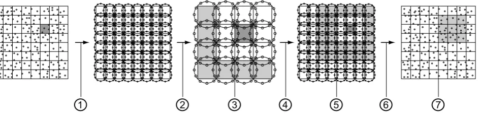
A schematic of the flow of calculation for the PMM is shown in Figure 1. The first figure from the left shows the FMM box structure at the highest box level, containing randomly distributed particles. The second figure shows the quadrature points, which are distributed on a spherical shell surrounding the boxes. The third figure shows the same, but for larger boxes. The light gray boxes in the third and fourth figure represent the boxes that interact with the dark gray box. The fifth figure shows the FMM box structure at the optimum level along with the particles. The figures are a two-dimensional representation of a three-dimensional calculation. The flow of calculation goes from left to right. The equations that are calculated in each step are as follows. The numbers correspond to those shown in Figure 1.
1. Equation 10 is calculated for the quadrature points on the circumscribing sphere
2. Makino’s method (Equation 7) is used to translate the vortex strength onto the larger spheres
3. Equation 10 is calculated for the quadrature points on the non-neighboring spheres 4. Anderson’s method (Equation 8) is used to
translate the potential onto the smaller spheres
5. Equation 10 is calculated for the quadrature points on the remaining non-neighboring spheres
6. Solve a system of equations given by Equation 10 to change the potential back into vortex strength. Then, calculate Equation 1 to obtain the velocity of all particles in the corresponding box
①
②
③
④
⑤
⑥
⑦
7. Calculate the remaining induced velocity using Equation 1 for all particles in the light gray box in the last figure.
In a standard FMM 1 would be the particle to multipole translation, 2 the multipole to multipole translation, 3 the multipole to local translation, 4 the local to local translation, 5 the multipole to local translation, 6 the local to particle translation, and 7 would be the direct summation.
The velocity calculation is performed for the direct summation, FMM, and PPM both with and without the MDGRAPE-3. N particles are randomly distributed in a box of [-π,π]3, and N is changed from 103 to 106. The order of multipole expansion in the FMM is set to p = 10 for all cases. For the PPM this corresponds to the use of 216 quadrature points in the spherical-t structure. All calculations were performed on a Intel Core2Quad (2.4 GHz) machine. Programs were multithreaded and vectorized by the intel fortran compiler. The CPU-time is shown for the different methods in Figure 2. Direct, FMM, PPM, are the results of the direct summation, FMM, and PPM. Figure 2a shows the CPU-time of each method when it is entirely calculated on the host machine. Figure 2b shows the CPU-time when the MDGRAPE-3 is used. The CPU-time for lower N deviates from the scaling laws, (especially in Figure 2b) because the relative computational overhead of insignificant portions of the program is dominant in these circumstances. The following observations can be made for calculations with large N.
The direct summation is over 200 times faster when calculated on the MDGRAPE-3. The FMM is about 13 times faster and the PPM is about 48 times faster when the MDGRAPE-3 is used. As shown in Figure 2a, the FMM is approximately 3 times faster than the PPM. However, in Figure 2b the PPM is slightly faster than the FMM for large N. The PPM can calculate both the multipole to local translation and the direct summation on the MDGRAPE-3, and should have a computational cost proportional to N. This is a large advantage over the standard FMM, where only the direct summation can be calculated.
The L2 error for the different methods is shown in Figure 3. The direct calculation is used as reference. The large error at small N is caused by the truncation of the smoothing functions for
non-neighboring boxes at the optimum level. In the present calculations the core radius of the vortex elements are set to 2πN-1/3 so that the overlap ratio is close to 1 for all N. The truncation error is largest at N = 103 where the inter-particle spacing is large compared to the optimum box size. The error becomes large again when the optimum box level changes, as shown near N ≈ 2 × 10⁴ and N ≈ 2 × 10⁵ for the FMM in Figure 3a.
3. VORTEX RING CALCULATION
3.1. Calculation Condition
The initial radiusof the vortex rings was R=1 while the cross-section radius was r = 0.05. The rings were inclined at an
(a)
(b)
angle θ = 15˚ relative to the z-axis (Figure 4). The Reynolds number based on the ring circulation was ReГ = Г/ν = 400. The initial condition had a
Gaussian distribution of vorticity in the cross section, as observed in experiments [19]. The vortex elements were distributed up to 3σg, where
σg is the standard deviation of the Gaussian distribution. This allows the diffusion to take place at the regions surrounding the vortex ring. Furthermore, the initial core radius of the vortex elements σ0 was set to twice the inter-particle spacing, which guarantees the overlap of elements for long calculations.
3.2. Movement of Vortex Elements
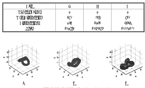
The collision of vortex rings is calculated using the second condition. The number of particles is changed for 105 ≤ N ≤ 107, while the Reynolds number is kept constant. The corresponding number of cross sections and number of elements per cross section are shown in Table 1. These numbers are determined by choosing a inter-particle distance that yields the total number of elements closest to N ≈ 105, N ≈ 106, and N ≈ 107. The movement of vortex elements for Case A is illustrated in Figure 5. The time t* = tГ/R2 is used hereafter, which is normalized by the circulation and radius of the vortex ring. At (a) t*=15, the two rings collide and begin to merge. At (b) t* = 30, the two rings merge into one. At (c) t* = 45 the vortex rings reconnect and form two new rings. One of the key features of the present calculation is that the vortex reconnection can be clearly observed. These results are supported by the fact that the present method considers the diffusion in the region surrounding the rings and also uses an accurate spatial adaption technique to ensure the convergence of the diffusion scheme for longer calculations. The reconnection observed here is also similar to the VIC results of Cottet, et al [13] and experimental results by Kida, et al [20].3.3. Effect of Spatial Resolution
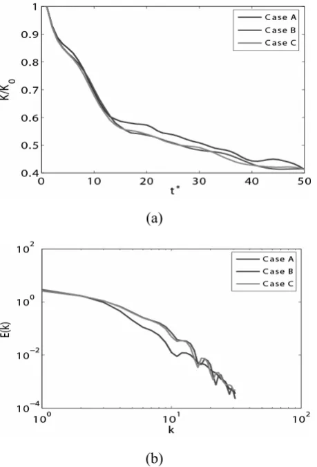
The necessity of a large number of particles to reproduce the quantitative aspects of the flow will be shown here. The kinetic energy K = 1/2ui2 is calculated from the velcoity of the vortex elements directly. The decay of kinetic energy is shown in Figure 6a to compare the results for different N. A quantitative difference between Case A and the other two is(a)
(b)
Figure 3. L2error for direct summation, FMM, and PPM with
and without MDGRAPE-3 (a) without MDGRAPE-3 (b) with MDGRAPE-3.
Figure 4. Initial condition for the computation of two vortex
clearly observed. Thus, as the number of elements is increased from N ≈ 105 to N ≈ 107 the energy decay shows convergent behavior with respect to N.
The energy spectra are calculated from the velocity distribution along the z-axis at selected times. The energy spectrum is shown in Figure 6b. The transfer and dissipation of kinetic energy determines the shape of the energy spectrum. Therefore, the agreement of the energy spectra reflects the soundness of the transfer and dissipation calculation. It is seen from Figure 6b that the energy spectra match when N ≥ 106.
4. CONCLUSIONS
The vortex method calculation is accelerated by the simultaneous use of the pseudo-particle method, Poisson integral method and a special purpose
computer MDGRAPE-3. The direct summation is over 200 times faster when calculated on the MDGRAPE-3. The FMM is about 13 times faster and the PPM is about 48 times faster when calculated on the MDGRAPE-3. The FMM is approximately 3 times faster than the PPM without the MDGRAPE-3. However, the PPM becomes faster than the FMM when it is calculated on the MDGRAPE-3. Consequently, PPM with MDGRAPE-3 is the fastest technique among others discussed above.
The collision of two vortex rings is selected as a test case. The reconnection of the vortex rings in the present calculation is similar to what is seen in experimental and DNS results. This is a result of the high precision of the stretching and diffusion calculations. The results of the calculations using more than 106 particles, not only reproduce the qualitative aspects of the reconnection, but also show nearly negligible discretization error. These features support the use of pure Lagrangian vortex methods in fairly complex 3-D flows.
TABLE 1. Breakdown of the Number of Elements.
Case A B C
Number of Rings N per Cross Section
Cross Sections Total
2 190 271 102980
2 418 1261 1054196
2 910 5677 10332140
(a) (b) (c)
5. REFERENCES
1. Greengard, L. and Rokhlin, V., “A Fast Algorithm for Particle Simulations”, J. Comput. Phys., Vol. 73, (1987),
325-348.
2. Salmon, J.K. and Warren, M.S., “Fast Parallel Tree Codes for Gravitational and Fluid Dynamical N-Body Problems”, Int. J. High Perf. Comput. Appl., Vol. 8,
(1994), 129-142
3. Winckelmans, G.S., Salmon, J.K., Warren, M.S., Leonard, A. and Jodoin, B., “Application of Fast Parallel and Sequential Tree Codes to Computing Three-Dimensional Flows with the Vortex Element and Boundary Element Methods”, ESAIM Proceedings,
Vol. 1, (1996), 225-240.
4. Collins, J.P., Dimas, A.A. and Bernard, P.S., “A Parallel Adaptive Fast Multipole Method for High Performance Vortex Method Based Simulations”, In: Proceedings of the ASME Fluids Engineering Division, FED,
Vol. 250, (1999).
5. Degond, P. and Mas-Gallic, S., “The Weighted Particle Method for Convection-Diffusion Equations. Part 1: The Case of an Isotropic Viscosity”, Math. Comput,
Vol. 53, (1989), 485-507.
6. Cottet, G.H., Michaux, B., Ossia, S. and VanderLinden, G., “A Comparison of Spectral and Vortex Methods in Three-Dimensional Incompressible Flows”, J. Comput. Phys., Vol. 175, (2002), 702-712.
7. Sbalzarini, I.F., Walther, J.H., Bergdorf, M., Hieber, S. E., Kotsalis, E.M. and Koumoutsakos, P., “PPM-A Highly Efficient Parallel Particle-Mesh Library for the Simulation of Continuum Systems”, J. Comput. Phys.,
Vol. 215, (2006), 566-588.
8. Narumi, T., Ohno, Y., Futatsugi, N., Okimoto, N., Suenaga, A., Yanai, R. and Taiji, M., “A High-Speed Special-Purpose Computer for Molecular Dynamics Simulations: MDGRAPE-3”, Proceedings of NIC Workshop, Vol. 34, (2006), 29-35.
9. Sugimoto, D., Chikada, Y., Makino, J., Ito, T., Ebisuzaki, T. and Umemura, M., “A Special-Purpose Computer for Gravitational Many-Body Problems”, Nature, Vol. 345,
(1990), 33-35.
10. Sheel, T.K., Yokota, R., Yasuoka, K. and Obi, S., “The Study of Colliding Vortex Rings using a Special-Purpose Computer and FMM”, Trans. Japan Soc. Comput. Eng. Sci., (2008), 0003.
11. Makino, J., “Yet Another Fast Multipole Method Without Multipoles-Pseudoparticle Multipole Method”,
J. Comput. Phys., Vol. 151, (1999), 910-920.
12. Anderson, C.R., “An Implementation of the Fast Multipole Method Without Multipoles”, SIAM J. Sci. Stat. Comput., Vol. 13, (1992), 923-947.
13. Cottet, G.H. and Koumoutsakos, P.D., “Vortex Methods”, Cambridge University Press, Cambridge, U.S.A., (2000), 245.
14. Winckelmans, G.S. and Leonard, A., “Contributions to Vortex Particle Methods for the Computation of Three-Dimensional Incompressible Unsteady Flows”, J. Comput. Phys., Vol. 109, (1993), 247-273.
15. Leonard, A., “Vortex Methods for Flow Simulations”,
J. Comput. Phys., Vol. 37, (1980), 289-335.
16. Barba, L.A., Leonard, A. and Allen, C.B., “Advances in Viscous Vortex Methods-Meshless Spatial Adaption Based on Radial Basis Function Interpolation”, Int. J. Num. Meth. Fluids, Vol. 47, (2005), 387-421.
17. Yokota, R., Sheel, T.K. and Obi, S., “Calculation of Isotropic Turbulence using a Pure Lagrangian Vortex Method”, J. Comput. Phys., Vol. 226, (2007),
1589-1606.
18. Sheel, T.K., Yasuoka, K. and Obi, S., “Fast Vortex Method Calculation using a Special-Purpose Computer”,
Comput. Fluids, Vol. 36, (2007), 1319-1326.
19. Shariff, K., Verzicco, R. and Orlandi, P., “A Numerical Study of Three-Dimensional Vortex Ring Instabilities: Viscous Corrections and Early Nonlinear Stage”, J. Fluid Mech., Vol. 279, (1994), 351-375.
20. Kida, S. and Takaoka, M., “Vortex Reconnection”,
Annu. Rev. Fluid Mech., Vol. 26, (1994), 169-189.
(a)
(b)
Figure 6. Effect of spatial resolution on the decay of kinetic