R E S E A R C H A R T I C L E
Open Access
Propensity score interval matching: using
bootstrap confidence intervals for
accommodating estimation errors of
propensity scores
Wei Pan
1*and Haiyan Bai
2Abstract
Background:Propensity score methods have become a popular tool for reducing selection bias in making causal
inference from observational studies in medical research. Propensity score matching, a key component of propensity score methods, normally matches units based on the distance between point estimates of the propensity scores. The problem with this technique is that it is difficult to establish a sensible criterion to evaluate the closeness of matched units without knowing estimation errors of the propensity scores.
Methods:The present study introducesinterval matchingusing bootstrap confidence intervals for accommodating estimation errors of propensity scores. In interval matching, if the confidence interval of a unit in the treatment group overlaps with that of one or more units in the comparison group, they are considered as matched units.
Results:The procedure of interval matching is illustrated in an empirical example using a real-life dataset from the Nursing Home Compare, a national survey conducted by the Centers for Medicare and Medicaid Services. The empirical example provided promising evidence that interval matching reduced more selection bias than did commonly used matching methods including the rival method, caliper matching. Interval matching’s approach methodologically sounds more meaningful than its competing matching methods because interval matching develop a more“scientific”criterion for matching units using confidence intervals.
Conclusions:Interval matching is a promisingly better alternative tool for reducing selection bias in making causal inference from observational studies, especially useful in secondary data analysis on national databases such as the Centers for Medicare and Medicaid Services data.
Keywords:Observational studies, Propensity score methods, Propensity score matching, Nearest neighbour
matching, Caliper matching, The bootstrap, Confidence intervals, Causal inference
Background
Observational studies are common in medical research because of practical or ethical barriers to random assign-ment of units (e.g., patients) into treatassign-ment conditions (e.g., treatment vs. comparison); consequently, observa-tional studies likely yield results with limited validity for causal inference due to selection bias resulted from non-randomization. To reduce selection bias, Rosenbaum
and Rubin [1] proposed propensity score methods for balancing the distributions of observed covariates between treatment conditions and, therefore, approximating a situ-ation that is normally achieved through randomizsitu-ation.
A propensity score is defined as the probability of a unit being assigned to the treatment group [1]. Propensity score methods normally comprise four major steps [2]:
1. Estimate a propensity score for each unit using a logistic regression of treatment conditions on covariates or other propensity score estimation methods [2,3];
* Correspondence:[email protected]
1
School of Nursing, Duke University, DUMC 3322, 307 Trent Drive, Durham, NC 27710, USA
Full list of author information is available at the end of the article
2. Match each unit in the treatment group with one or more units in the comparison group based on the closest distance between their propensity scores; 3. Evaluate the matching quality in terms of how much
selection bias is reduced; and
4. Conduct intended outcome analysis on the matched data or on the original data with propensity score adjustment or weighting.
Although propensity score methods have become in-creasingly popular in medical research over the past three decades as an effective tool for reducing selection bias in making causal inference based on observational data, propensity score matching (PSM), as a crucial step in propensity score methods, still has limitations [2]. For example, in the existent PSM techniques, matching is done primarily based on the distance betweenpoint esti-matesof propensity scores, and thus, it is difficult to es-tablish a meaningful criterion to evaluate the closeness of the matched units without knowing the estimation er-rors (or standard erer-rors) of the estimated propensity scores. Previously, Cochran and Rubin [4] proposed cali-per matching, which uses a calicali-per band (e.g., a pre-specified distance between propensity scores) to avoid “bad”matches that are not close enough. Unfortunately, a caliper band is expressed as a proportion to the pooled standard deviation of propensity scores across all the units, and therefore, it isunit-invariant; that is, a caliper band takes the same value for all the units. Therefore, a caliper band does not possess a feature that can gauge theunit-specific standard error of the estimated propen-sity score for each individual unit.
The purpose of the present study was to extend caliper matching to a new matching technique,interval matching, by using unit-specific bootstrap confidence intervals (CIs) [5] for gauging the standard error of the estimated propen-sity score for each unit. In interval matching, if the confi-dence interval of a unit in the treatment group overlaps with that of one or more units in the comparison group, they are considered as matched units. In the present study, the procedure of interval matching is illustrated in an empirical example using a real-life sample from a publicly available database of the Nursing Home Compare [6], a national survey conducted by the Centers for Medicare and Medicaid Services (CMS) in the United States.
Methods PSM assumptions
Suppose one has N units. In addition to a response valueYi, each ofNunits has a covariate value vectorXi
= (Xi1,…,XiK)′, wherei= 1, …,N, andKis the number
of covariates. Let Ti be the treatment condition. Ti= 1
indicates that unitiis in the treatment group andTi= 0
the comparison group. Rosenbaum and Rubin [1]
defined a propensity score for unit i as the probability of the unit being assigned to the treatment group, con-ditional on the covariate vectorXi; that is,
pð Þ ¼Xi Pr Tð i¼1jXiÞ: ð1Þ
PSM is based on the following two strong ignorability assumptions in treatment assignment [1]: (1) (Y1i,Y0i)⊥ Ti| Xi; and (2) 0 <p(Xi) < 1. The first assumption states
a condition that treatment assignment Ti and response
(Y1i, Y0i) are conditionally independent, given Xi; the
second one ensures a common support between the treatment and comparison groups.
Rosenbaum and Rubin [1] further demonstrated in their Theorem 3 that ignorability conditional on Xi
implies ignorability conditional onp(Xi); that is,
Y1i;Y0i
ð Þ⊥TijXi⇒ðY1i;Y0iÞ⊥Tijpð ÞXi : ð2Þ
Thus, under the assumptions of the strong ignorability in treatment assignment, if a unit in the treatment group and a corresponding matched unit in the comparison group have the same propensity score, the two matched units will have, in probability, the same value of the co-variate vector Xi. Therefore, outcome analysis on the
matched data after matching tends to produce unbiased estimates of treatment effects due to reduced selection bias through balancing the distributions of observed co-variates between the treatment and comparison groups [1, 2, 7]. In practice, the logit of propensity score,l(Xi) =
ln{p(Xi)/[1 – p(Xi)]}, rather than the propensity score p(Xi) itself, is commonly used becausel(Xi) has a better
property of normality than doesp(Xi) [1].
PSM methods
The basis of PSM is nearest neighbor matching [8], which matches unit iin the treatment group with unitj
in the comparison group with the closest distance be-tween the two units’ logit of their propensity scores expressed as follows:
d ið Þ ¼;j minj lð ÞXi –l Xj
: ð3Þ
Alternatively, caliper matching [4] matches unit i in the treatment group with unitjin the comparison group within a pre-set caliper bandb; that is,
d ið Þ ¼;j minj lð ÞXi –l Xj <b
: ð4Þ
Based on Cochran and Rubin’s work [4], Rosenbaum and Rubin [8] recommend b equals 0.25 of the pooled standard deviation (SD) of the propensity scores. Austin [9] further asserted that b= 0.20 ×SD of the propensity scores is the optimal caliper bandwidth.
metric matching within a propensity score caliper) [8] are two additional matching techniques similar to nearest neighbor matching and caliper matching, respectively, but use a diffident distance measure. In Mahalanobis metric matching, unit i in the treatment group is matched with unit j in the comparison group with the closest Mahalanobis distance measured as follows:
d ið Þ ¼;j minj Dij ; ð5Þ
whereDij= (Zi′ –Zj′)′S−1(Zi′ –Zj′),Z•(•=ior j) is a
new vector (X•, l(X•)), and S is the sample
variance-covariance matrix of the vector for the comparison group. Mahalanobis caliper matching is a variant of Mahalanobis metric matching and it uses
d ið Þ ¼;j minj Dij<b
; ð6Þ
where the selection of the caliper band bis the same as in caliper matching.
Data reduction after matching is a common and inev-itable phenomenon in PSM. Loss of data in the compari-son group seems a problem, but what we lose is unmatched cases that are assumed to potentially cause selection bias, and therefore, those unmatched units would have a negative impact on estimation of treatment effects. The matched data that may have a smaller sam-ple size will, however, produce more valid (or less biased) estimates than do the original data. It is true that if we have small samples, which is not uncommon in medical research, PSM may not be applicable in such sit-uations, but PSM is particularly useful in secondary data analysis on national databases such as the CMS data.
PSM algorithms
All aforementioned PSM methods can be implemented by using eithergreedy matching oroptimal matching al-gorithm [10]. Both matching alal-gorithms usually produce similar matched data when the size of the comparison group is large; whereas optimal matching gives rise to smaller overall distances within matched units [11, 12]. All the matching techniques, either using greedy match-ing or optimal matchmatch-ing, are based on the distance be-tween point estimates of propensity scores. The problem with this approach is that it is difficult to establish a meaningful criterion to evaluate the closeness of the matched units without knowing the standard errors of the estimated unit-specific propensity scores. Simply put, without knowing the standard errors of l(Xi) and l(Xj), we do not know ifl(Xj) in the comparison group is
the best matched score with l(Xi) in the treatment
group. In other words, a score a little smaller than l(Xj)
might be a better matched one withl(Xi); or conversely, l(Xj) might be matched better with a score a little larger
thanl(Xi).
Although caliper matching, one of the most effective matching methods [13–15], uses a caliper band to avoid “bad”matches, a caliper band is fixed (or unit-invariant) and cannot capture the unit-specific standard error of the estimated propensity score for each unit. Therefore, a new matching technique is needed for gauging standard errors of propensity scores.
Interval matching
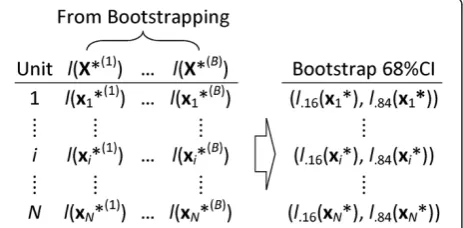
Interval matching extends caliper matching for accom-modating the estimation error (or standard error) of the estimated propensity score by establishing a CI of the estimated propensity score for each unit. In interval matching, if the CI of a unit in the treatment group overlaps with that of one or more units in the compari-son group, they are considered as matched units. Because the true distribution of propensity scores is unknown, the bootstrap [5] is utilized for obtaining a unit-specific CI for each unit. The bootstrap is a statis-tical method of assessing the accuracy (e.g., standard errors and CIs) of sample estimates to population pa-rameters, based on the empirical distribution of sample estimates from random resamples of a given sample whose distribution is unknown.
Let {X1,…,XN} be a random sample of sizeNfrom an
unknown distribution F; θ(F) is a parameter of interest. The specific procedure of the bootstrap for computing a CI of the parameter estimate, [θ^a=2 (X1, …, XN), ^θ1−a=2 (X1, …, XN)], where (1 -α) is the confidence level,
con-sists of the following four steps:
1. Obtain a bootstrap sample {X1*,…,XN*} that is
randomly resampled with replacement from the empirical distributionFNrepresented by the original sample {X1,…,XN};
2. Calculate the parameter estimate^θ(X1*,…,XN*) for
the quantityθ(FN) =θ(X1,…,XN);
3. Repeat the same independent resampling-calculating schemeBtimes (typically 500 times), resulting inB bootstrap estimatesθ^(X1*(b),…,XN*(b)),b= 1,…,B,
which constitute an empirical distribution (or sam-pling distribution) of the estimateθ^(X1,…,XN); and
4. Obtain the estimated CI of the parameter estimate, [θ^a=2(X1,…,XN),θ^1−a=2(X1,…,XN)], by computing
the (α/2)th and (1–α/2)th percentiles of the sampling distribution,^θa=2(X1*,…,XN*) and^θ1−a=2
(X1*,…,XN*).
matrix (X1, …, XN)′, resulting in B bootstrap samples
(T(b),X(b)), whereX(b)= (X1*(b),…,XN*(b))′, b= 1, …, B.
Second, a logistic regression (or other propensity score estimation model) is repeatedly applied to each of theB
bootstrap samples, resulting inB propensity scores for each unit i (i= 1, …, N): p(Xi*(1)), …, p(Xi*(B)); then,
their logit,l(Xi*(1)), …, l(Xi*(B)), are calculated. Last, for
each unit i, a CI at certain confidence level (e.g., 68 %CI) is obtained by calculating the corresponding percentiles of the sampling distribution of the logit ofB
bootstrap propensity scores. Specifically, an estimated bootstrap 68 %CI for the logit of the propensity score of unit i would be [l.16(Xi*), l.84(Xi*)] (see Fig. 1 for an
illustration).
Once a CI of the estimate of the logit of propensity score is obtained for each unit, interval matching can be conducted by examining whether the CI for a unit in the treatment group overlaps with that for one or more units in the comparison group. In other words, if the two CIs overlap; that is,
l:16ðXiÞ;l:84ðXiÞ
½ ∩ l:16 Xj
;l:84 Xj
≠∅; ð7Þ
the two units are taken as matched units. In practice, one can do either 1:1 or 1:K interval matching. In 1:1 interval matching, one needs to take only one unit that has the closest distance, as defined by the matching method (e.g., Equation 3 for nearest neighbor matching and Equation 6 for Mahalanobis caliper matching), between the logit of the propensity scores among all the units in the comparison group whose CIs overlap with that of the unit in the treatment group. If there are two or more units in the comparison group within the over-lap having the same closest distance, the program will randomly select one as the matched unit. In 1:Kinterval matching, one can simply take K closest units in the comparison group whose CIs overlap with that of the unit in the treatment group.
It is worth noting that using the logit of propensity scorel(Xi) is particularly important in interval matching
because the distribution of logitl(Xi) is more symmetric
than the propensity score p(Xi); therefore, interval
matching based on logit l(Xi) will be more balanced in
terms of matching from both sides (left or right) of the distribution of logitl(Xi).
Results
The procedure of interval matching is illustrated in an empirical example that was stemmed from Lutfiyya, Gessert, and Lipsky’s comparative study [16]. They com-pared nursing home quality between rural and urban facilities using the CMS Nursing Home Compare data in 2010 on the past performance of all Medicare- and Medicaid-certified nursing homes in the United States [6]. The data were downloaded from the CMS Nursing Home Compare Website on more than 10,000 nursing homes with the geographical location (rural vs. urban) information extracted from the 2003 rural–urban county continuum codes developed by the Economic Research Service of the United States Department of Agriculture [17]. Quality ratings on nursing home performance were measured on three domains: health inspection, staffing, and quality measures [6]. An overall rating was also computed as a weighted average of the three domains. Lutfiyya, Gessert, and Lipsky [16] concluded that rural nursing home quality was not comparable to that of urban nursing homes with mixed findings: rural nursing homes had significantly higher quality ratings on the overall rating (p< .001) and health inspections rating (p
< .001) than did urban nursing homes, but significantly lower on the quality measures rating (p< .001) than did urban nursing homes; while there was no significant dif-ference in nursing staffing rating (p= .480) between rural and urban nursing homes.
The problem in Lutfiyya, Gessert, and Lipsky’s study [16] is that the geographical location (rural vs. urban) of nursing homes was not randomly assigned, and conse-quently, unbalanced background characteristics of nurs-ing homes created potential selection bias between rural and urban nursing homes. Propensity score methods would be an appropriate technique to deal with this selection bias problem in such observational study.
Data source
For illustration purposes only, the data used in this em-pirical example were a 50 % random sample from the same publicly available database, the CMS Nursing Home Compare in 2010. The sample data consisted of total N= 6,317 nursing homes (nR= 1,990 rural nursing
homes and nU= 4,327 urban nursing homes) with 74
covariates of the ownership and size of nursing homes, qualification of nursing staff, and safety measures (see Additional file 1 for a full list of the 74 covariates). The 74 covariates were hypothesized to be related to the quality ratings and/or group assignment and, thus, all Fig. 1The procedure of obtaining bootstrap 68 %CIs of the logit of
included in this empirical example. Due to the scope of this example and the space limit, general guidelines on covariate selection is not discussed here but available elsewhere [18].
It is also worth noting that due to the purpose of this example which is to illustrate the procedure of interval matching, replicating Lutfiyya, Gessert, and Lipsky’s study [16] of testing the difference in nursing home quality between rural and urban nursing homes was not the main focus of this example; instead, this example focused on evaluating the effectiveness of interval matching along with other commonly used PSM methods for reducing selection bias (or balancing covariates) between rural and urban nursing homes. Also, without loss of generality, 1:1 interval matching was illustrated; the present example can be easily extended to 1:K interval matching without any difficulty.
Propensity score bootstrap CIs
Five hundred bootstrap samples were first resampled from the data using SAS® PROC SURVEYSELECT [19], and then for each of the 500 bootstrap samples, logistic regression of rural vs. urban nursing homes on the 74 covariates was conducted to obtain the probability (or the propensity score) of being a rural nursing home for each nursing home. There are some other propensity score estimation models, but without loss of generality, logistic regression was used in this example for illustra-tion purposes only. Next, the logit of the propensity score for each nursing home was computed, and boot-strap 50 %, 68 %, and 95 %CIs of the logit for each nurs-ing home were constructed by calculatnurs-ing the 25th percentile and the 75th percentile, the 16th percentile and the 84th percentile, and the 2.5th percentile and the 97.5th percentile, respectively, of the 500 bootstrap logit values. The purpose of computing the bootstrap CIs at different confidence levels was to examine the effect of the confidence level on the selection bias reduction in interval matching. Analogous to caliper bandwidth in caliper matching, the average of the half widths of the 6,317 bootstrap CIs was 0.20, ranging from 0.06 to 7.96 with a standard deviation of 0.19, for 50 %CIs; 0.29, ran-ging from 0.09 to 11.03 with a standard deviation of 0.29, for 68 %CIs; and 0.59, ranging from 0.20 to 26.35 with a standard deviation of 0.70, for 95 %CIs.
Matching and evaluation of matching quality
The effectiveness of interval matching for reducing selection bias was evaluated along with the basic neighbor matching and the related caliper matching as well as other two commonly used matching methods, Mahalanobis caliper matching and optimal matching. All but optimal matching methods were implemented using a modified SAS® Macro based on Coca-Perraillon [20]. The optimal
matching was conducted using an R package, MatchIt
[12]. The pooled SDof the logit of the propensity scores
l(Xi) (i= 1, 2,…, 6,317) was 1.86; the caliper band for
cali-per matching in this example was b= 0.20 ×SD= 0.20 × 1.86 = 0.37.
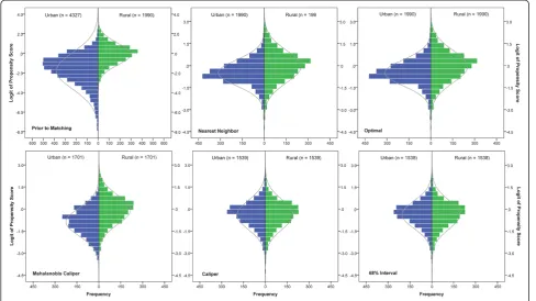
Figure 2 displays the distributions of the logit of pro-pensity scores between the rural and urban nursing homes prior to and post matching. By visually inspecting the distributions of the logit of propensity scores, it can be seen that interval matching as well as caliper match-ing did better in balancmatch-ing the distributions between the rural and urban nursing homes than did nearest neigh-bor matching, optimal matching, and Mahalanobis cali-per matching. Three statistical criteria were also used to evaluate the effectiveness of the matching methods in balancing the distributions. They were the mean differ-ence (or selection bias [B]), the standardized bias (SB), and the percent bias reduction (PBR).
The selection bias for each covariateXk(k= 1,…,K) is
the mean difference between the rural and urban nursing homes as follows:
B¼M1ð ÞXk –M0ð ÞXk ; ð8Þ
where M1(Xk) is the mean of the covariate for the rural
nursing homes and M0(Xk) is the mean of the covariate
for the urban nursing homes. The SB associated with each covariate was defined by Rosenbaum and Rubin [8] as follows:
SB¼ ffiffiffiffiffiffiffiffiffiffiffiffiffiffiffiffiffiffiffiffiffiffiffiffiB
V1ð ÞþXk V0ð ÞXk
2
q 100%; ð9Þ
where V1(Xk) is the variance of the covariate for the
rural nursing homes and V0(Xk) is the variance of the
covariate for the urban nursing homes. According to Caliendo and Kopeinig [21], if the absoluteSBis reduced to 5 % or less after matching, the matching method is considered effective in reducing selection bias. ThePBR
on the covariate was proposed by Cochran and Rubin [4] and it can be expressed as follows:
PBR¼Bprior to matchingj j−Bpost matching Bprior to matching
100%: ð10Þ
Note that the original expression ofPBRin the litera-ture [2, 4, 22, 23] did not impose the absolute values for
B; here PBR (Equation 10) includes the absolute values to make the criterion more meaningful because both positive and negative Bs indicate unbalanced distribu-tions of the covariate.
Table 1, we can see that selection bias prior to matching was evident in that the average of the 74 absoluteSBs was 16.22 %. In addition, the selection bias is also indicated by the severely unbalanced distributions of the logit of the pro-pensity scores withSB= 78.73 %.
The results of applying nearest neighbor matching, optimal matching, Mahalanobis caliper matching, caliper matching, and three interval matching methods are also presented in Table 1. First of all, the average of absolute
SBs, and average PBRs across all 74 covariates demon-strated that the three interval matching methods as well as
caliper matching were superior to all other matching methods by all means. Furthermore, by examining the stat-istical criteria for the logit of propensity scores—“arguably the most important variable” ([8], p. 36) in balancing the distributions of the covariates, the data suggested that 68 % interval matching outperformed caliper matching because the interval matching removed 99.64 % of the selection bias with remaining SB=−0.46 %, compared to 98.41 % for caliper matching (remaining SB= 1.96 %). In addition, this favorable phenomenon to 68 % interval matching was also echoed by the average PBR across all covariates
Table 1A summary of selection bias prior to matching and bias reduction post matching
Matching Method Sample Size SBfor Logit of PS (%) PBRfor Logit of PS (%) Average of AbsoluteSB across 74 Covariates (%)
Average ofPBRacross 74 Covariates (%)
Prior to Matching nR= 1990nU= 4327 78.73 — 16.22 —
Post Matching
Nearest Neighbor nR=nU= 1990 30.23 75.21 4.84 53.32
Optimal nR=nU= 1990 30.23 75.21 4.91 55.15
Mahalanobis Caliper nR=nU= 1701 61.04 51.79 10.16 25.70
Caliper nR=nU= 1539 1.96 98.41 1.00 76.78
50 % Interval nR=nU= 1483 −2.89 97.69 1.43 76.50
68 % Interval nR=nU= 1538 −0.46 99.64 1.25 79.24
95 % Interval nR=nU= 1713 9.52 92.55 1.33 79.12
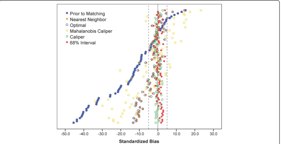
(PBR = 79.24 %), compared toPBR = 76.78 % for caliper matching; only the average SB of 68 % interval matching was slightly larger than but comparable to that of caliper matching (1.25 % vs. 1.0 %). Individual covariate balancing is also summarized in a graphical display (see Fig. 3) ofSBs prior to and post the five matching methods. It is clearly seen that both interval matching and caliper matching sig-nificantly reduced more selection bias than did other matching methods because all theSBs of interval matching and caliper matching were within 5 %; whereas a sub-stantial amount of the SBs of other matching were larger than 5 %.
Discussion
The present study used bootstrap CIs at 50 %, 68 %, and 95 % confidence levels in the empirical example which demonstrated that 68 %CIs performed the best among the three (see Table 1) and to some extent better than caliper matching. When the empirical distribution of the logit of the estimated propensity score is normally dis-tributed, a 68 %CI will be a range of ±1 standard error away from the mean; whereas the caliper band in caliper matching uses 0.20 standard deviation of the logit of the propensity score. A higher level of percentage (i.e., confi-dence level) (>68 %) will lead to more possible matched units and a lower level of percentage (<68 %) will lead to more rigid matching and, thus, possible fewer matched units. In practice, researchers can determine what per-centage of CI to use for accommodating a different size
of a comparison group. In general, a smaller percentage of CI may be used for a larger comparison group. In addition, 500 bootstrap samples were used in the empir-ical example. If some units are not selected in a boot-strap sample, a larger number of bootboot-strap samples may be used to avoid the situation where few bootstrap pro-pensity scores are obtained for the unit.
As a side note, the difference in nursing home quality between rural and urban homes were compared using the matched data with 68 % interval matching, and the results (see Table 2) are different from those of Lutfiyya, Gessert, and Lipsky’s study [16]. Specifically, Table 2 shows that rural nursing homes had lower quality ratings on all the ratings than urban nursing homes, but only quality measures rating was significant (p< .001).
Conclusions
The normal procedure of current PSM is to match each unit in the treatment group with one or more units in the comparison group based on the distance between the point estimates of propensity scores. Unfortunately, the point estimates cannot capture estimation errors (or standard errors) of propensity scores. The present study proposed interval matching using bootstrap CIs for ac-commodating unit-specific standard errors of (the logit of ) propensity scores. Interval matching’s approach methodologically sounds more meaningful than its com-peting matching methods because interval matching develop a more “scientific” criterion for matching units using confidence intervals.
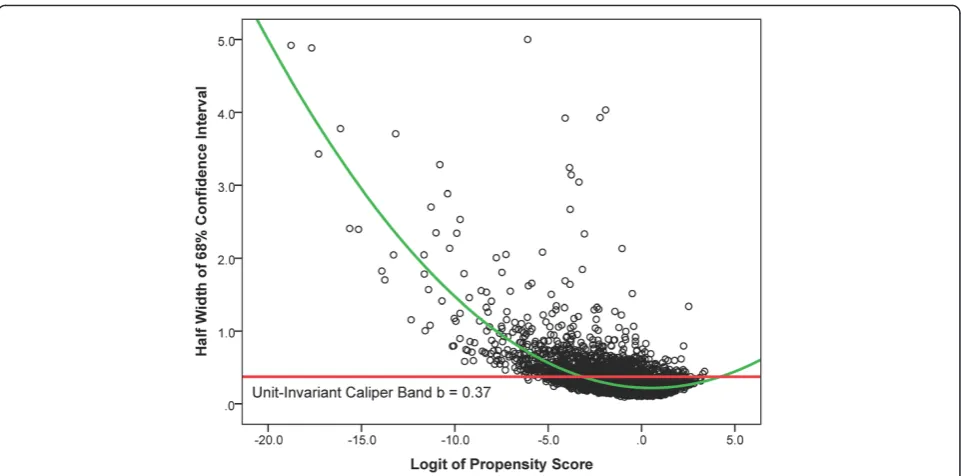
Besides accommodating standard errors of propensity scores using confidence intervals, interval matching has another methodologically sound property. That is, CIs of the logit of estimated propensity scores in relatively sparse areas where it is less likely to find matched units would be wider than those in the area with more dense data where it is more likely to find matched units. This curve-linear relationship between the width of CIs and the density of the distribution of the logit of propensity scores may lead to more matched units in sparse areas to balance out the area with more dense data (see Fig. 4); whereas caliper matching has a fixed caliper bandwidth (e.g., b= 0.37 for this empirical example) for all the values of the logit of propensity scores regardless the density of the distribution of the logit of propensity scores.
Because these beneficial properties of interval match-ing, the empirical example demonstrated that interval matching is not only a viable alternative to caliper
matching, but also produced promisingly more balanced data than did all other matching methods including cali-per matching.
It is true that the computation in interval matching is somewhat more labor intensive than that in other PSM methods. However, it should not be a problem in today’s fast computing technology, which makes the encour-aging results in interval matching overweigh its intensive computation.
In future research, we would like to further explore the effectiveness of interval matching on reducing selection bias in a simulation study by creating different scenarios, such as 1:Kmatching, matching with replacement, sample size ratio of treatment group to comparison group, and size of common support between treatment and comparison groups. In addition to the effectiveness of interval matching on reducing selection bias, it would be also desirable to examine the effectiveness of interval matching on reducing estimation bias for treatment effects under various scenar-ios, comparing with some other matching techniques mainly for bias reduction in estimating treatment effects, such as full matching, subclassification, kernel match-ing (or difference-in-deference matchmatch-ing), as well as different propensity score estimation models.
In sum, interval matching possess sound methodological properties and is a promisingly better alternative tool for reducing selection bias in making causal inference from observational studies, especially helpful in secondary data analysis on national databases such as the CMS data as demonstrated in the empirical example.
Table 2Means (standard deviations) of nursing home quality ratings and independent samplest-test on the matched data with 68 % interval matching (nrural=nurban= 1,538)
Nursing Home Quality Rating
Geographical Location t p
Rural Urban
Overall rating 3.06(1.30) 3.12(1.31) −1.188 .235 Health inspections rating 2.90(1.26) 2.91(1.31) −0.126 .899
Nurse staffing rating 2.98(1.22) 3.01(1.21) −0.740 .459
Quality measures rating 3.14(1.23) 3.30(1.20) −3.535 < .001
Additional files
Additional file 1:A list of the 74 covariates in the example data
from the CMS nursing home compare database.(DOCX 18 kb)
Additional file 2:Selection bias prior to matching and bias
reduction post matching for all 74 covariates.(XLS 62 kb)
Abbreviations
B:mean difference (or selection bias); CI: confidence interval; CMS: the Centers for Medicare and Medicaid Services; PBR: percent bias reduction; PSM: propensity score matching; SB: standardized bias; SD: standard deviation.
Competing interests
The authors declare that they have no competing interests.
Authors’contributions
WP developed the methods, conducted the study, and wrote the initial draft of the manuscript. HB conceived of the study, participated in its design, and helped to draft the manuscript. All authors read and approved the final manuscript.
Acknowledgements
We would like to thank Diane Holditch-Davis for the content review on the example of the Nursing Home Compare and Judith C. Hays for the language editorial review.
Author details
1
School of Nursing, Duke University, DUMC 3322, 307 Trent Drive, Durham, NC 27710, USA.2Department of Educational and Human Sciences, University
of Central Florida, PO Box 161250, Orlando, FL 32816, USA.
Received: 8 November 2014 Accepted: 13 July 2015
References
1. Rosenbaum PR, Rubin DB. The central role of the propensity score in observational studies for causal effects. Biometrika. 1983;70(1):41–55. 2. Pan W, Bai H, editors. Propensity score analysis: Fundamentals and
developments. New York, NY: The Guilford Press; 2015.
3. McCaffrey DF, Ridgeway G, Morral AR. Propensity score estimation with boosted regression for evaluating causal effects in observational studies. Psychological methods. 2004;9(4):403–25.
4. Cochran WG, Rubin DB. Controlling bias in observational studies: A review. Sankhyā: The Indian Journal of Statistics, Series A. 1973;35(4):417–46. 5. Efron B, Tibshirani RJ. An introduction to the bootstrap. New York, NY: CRC
Press LLC; 1998.
6. Design for Nursing Home Compare five-star quality rating system: Technical users’guide [http://www.cms.gov/Medicare/Provider-Enrollment-and-Certification/CertificationandComplianc/Downloads/usersguide.pdf] 7. Ho DE, Imai K, King G, Stuart EA: Matching as nonparametric preprocessing
for reducing model dependence in parametric causal inference.Political Analysis2007.
8. Rosenbaum PR, Rubin DB. Constructing a control group using multivariate matched sampling methods that incorporate the propensity score. The American Statistician. 1985;39(1):33–8.
9. Austin PC. Optimal caliper widths for propensity-score matching when estimating differences in means and differences in proportions in observational studies. Pharmaceutical statistics. 2011;10(2):150–61. 10. Rosenbaum PR. Optimal matching for observational studies. Journal of the
American Statistical Association. 1989;84(408):1024–32.
11. Gu XS, Rosenbaum PR. Comparison of multivariate matching methods: Structures, distances, and algorithms. Journal of Computational and Graphical Statistics. 1993;2(4):405–20.
12. Ho DE, Imai K, King G, Stuart EA. MatchIt: Nonparametric preprocessing for parametric causal inference. Journal of Statistical Software. 2011;42(8):1–28. 13. Austin PC. An Introduction to propensity score methods for reducing the
effects of confounding in observational studies. Multivariate behavioral research. 2011;46(3):399–424.
14. Bai H. A comparison of propensity score matching methods for reducing selection bias. International Journal of Research & Method in Education. 2011;34(1):81–107.
15. Guo S, Barth RP, Gibbons C. Propensity score matching strategies for evaluating substance abuse services for child welfare clients. Children and Youth Services Review. 2006;28(4):357–83.
16. Lutfiyya MN, Gessert CE, Lipsky MS. Nursing home quality: A comparative analysis using CMS Nursing Home Compare data to examine differences between rural and nonrural facilities. Journal of the American Medical Directors Association. 2013;14(8):593–8.
17. Rural–urban continuum codes [http://www.ers.usda.gov/data-products/ rural-urban-continuum-codes/documentation.aspx]
18. Brookhart MA, Schneeweiss S, Rothman KJ, Glynn RJ, Avorn J, Stürmer T. Variable selection for propensity score models. Am J Epidemiol. 2006;163(12):1149–56.
19. Don’t be loopy: Re-sampling and simulation the SAS® way [http://www2. sas.com/proceedings/forum2007/183-2007.pdf]
20. Local and global optimal propensity score matching [http://www2.sas.com/ proceedings/forum2007/185-2007.pdf]
21. Caliendo M, Kopeinig S. Some practical guidance for the implementation of propensity score matching. Journal of Economic Surveys. 2008;22(1):31–72. 22. Rubin DB. Multivariate matching methods that are equal percent bias
reducing, II: Maximums on bias Rreduction for fixed sample sizes. Biometrics. 1976;32(1):121–32.
23. Rubin DB. Multivariate matching methods that are equal percent bias reducing, I: Some examples. Biometrics. 1976;32(1):109–20.
Submit your next manuscript to BioMed Central and take full advantage of:
• Convenient online submission
• Thorough peer review
• No space constraints or color figure charges
• Immediate publication on acceptance
• Inclusion in PubMed, CAS, Scopus and Google Scholar
• Research which is freely available for redistribution