!
"
#"#
$ % %#
&
'
((( )
A Crossover Probability Distribution in Genetic Algorithm Under process Scheduling
Problem
Er.Rajiv Kumar*
PhD. Scholar Singhania University Jhunjhunu,Rajasthan, INDIA [email protected]
Er Sanjeev Gill
Lecturer, Civil Engg. Deptt.
Global research Institute of Management & Technology Radaur Yamuna Nagar,Haryana
Er. Ashwani Kaushik
Lecturer,Mechanical Engg Deptt. N.C.College of Engineering Israna, Panipat
Abstract: This paper describe the effect of crossover probability on the convergence of genetic algorithm. Genetic Algorithm have been designed as general purpose optimization method. The power of the genetic algorithm is depends upon the proper use of their operators such as selection, crossover and mutation. In this paper we apply the varying crossover probability under the operating system process scheduling problem. The diversity of the population of the individuals are determine by the probability of crossover in the genetic algorithm. Crossover is work as a diversifier for the population of solution in the genetic algorithm. The experiments shows that as the probability of cross over increase more easily the GA adapt to the problem and converge to the best solution state.
Keywords: Genetic algorithm, NP-hard, Process Scheduling, Crossover
I. INTRODUCTION
Genetic Algorithms (GAs) are robust and intelligent search method. The most important charactersitc of the GA is its adaptability according to the problem on which it is applied they are based on the genetic processes of biological organisms. Over many generations, natural populations evolve according to the principles of natural selection and “survival of the fittest", first clearly stated by Charles Darwin in The Origin of Species. By mimicking this process, genetic algorithms are able to evolve" solutions to real world problems, if they have been suitably encoded. Then it can find out the best solution to the problem .
The principles of GAs were first laid down by Professor Holland [1], and are well described in many texts (e.g. [2], [3], [4], [5]) GAs simulate those processes in natural populations which are essential to evolution. Exactly which biological processes are essential for evolution, and which processes have little or no role to play is still a matter for research; but the foundations are clear. In nature, individuals in a population compete with each other for resources such as food, water and shelter.
Also, members of the same species often compete to attract a mate. Those individuals which are most successful in surviving and attracting mates will have relatively larger numbers of offspring. Poorly performing individuals will produce few of even no offspring at all. This means that the genes from the highly adapted, or “fit" individuals will spread to an increasing number of individuals in each successive generation. The combination of good characteristics from differrent ancestors can sometimes produce “super fit" offspring, whose fitness is greater than that of either parent. In this way, species evolve to become more and better suited to their environment.
GAs use a direct analogy of natural behavior. They work with a population of “individuals", each representing a possible solution to a given problem. Each individual is assigned a “fitness score" according to how good a solution to the problem it is. The power of GAs comes from the fact that the technique is robust, and can deal successfully with a wide range of problem areas, including those which are difficult for other methods to solve. GAs are not guaranteed to find the global optimum solution to a problem, but they are generally good at finding” acceptably good" solutions to problems “acceptably quickly". Where specialized techniques exist for solving particular problems, they are likely to out-perform GAs in both speed and accuracy of the final result. The main ground for GAs, then, is in difficult areas where no such techniques exist. Even where existing techniques work well, improvements have been made by hybridizing them with a GA.
II. METHODOLOGY
A. Coding
It is assumed that a potential solution to a problem may be represented as a set of parameters .In the process scheduling problem we use permutation coding technique. These parameters (known as genes) are joined together to form a string of values (often referred to as a chromosome). (Holland [1] first showed, and many still believe, that the ideal is to use
Chromosome 1 1101100100110110
Chromosome 2 1101111000011110
A binary alphabet for the string. For example, if our problem is to maximize a function of three variables, F(x; y; z), we might represent each variable by a 10-bit binary number (suitably scaled). Our chromosome would therefore contain three genes, and consist of 30 binary digits. In our problem we take five jobs and they have number 1,2,3,4 and 5. Also with this job number each job is associated with their job process time .when we arrange randomly these job they will make a particular schedule then we apply fitness function which find out the merit of the solution. In genetics terms, the set of parameters represented by a particular chromosome is referred to as a genotype.
The genotype contains the information required to construct an organism which is referred to as the phenotype.
B. Initialization
Initially many individual solutions are randomly generated to form an initial population. The population size depends on the nature of the problem, but typically contains several hundreds or thousands of possible solutions. Traditionally, the population is generated randomly, covering the entire range of possible solutions (the search space). Occasionally, the solutions may be "seeded" in areas where optimal solutions are likely to be found.
C. Selection
Main article: Selection (genetic algorithm) during each successive generation, a proportion of the existing population is selected to breed a new generation. Individual solutions are selected through a fitness-based process, where fitter solutions (as measured by a fitness function) are typically more likely to be selected. Certain selection methods rate the fitness of each solution and preferentially select the best solutions. Other methods rate only a random sample of the population, as this process may be very time-consuming. Most functions are stochastic and designed so that a small proportion of less fit solutions are selected. This helps keep the diversity of the population large, preventing premature convergence on poor solutions. Popular and well-studied selection methods include roulette wheel selection and tournament selection.
D. Reproduction
During the reproductive phase of the GA, individuals are selected from the population and recombined, producing offspring which will comprise the next generation. Parents are selected randomly from the population using a scheme which favors the more _t individuals. Good individuals will probably be selected several times in a generation; poor ones may not be at all. Having selected two parents, their chromosomes are recombined, typically using the mechanisms of crossover and mutation. The most basic forms of these operators are as follows:
[image:2.612.330.550.53.200.2]Crossover takes two individuals, and cuts their chromosome strings at some randomly chosen position, to produce two \head" segments, and two “tail" segments. The tail segments are then swapped over to produce two new full length chromosomes (see Figure 2). The two offspring each inherit some genes from each parent. This is known as single point crossover. Crossover is not usually applied to all pairs of individuals selected for mating.
Figure 2. Single Point Crossover
A random choice is made, where the likelihood of crossover being applied is typically between 0.6 and 1.0. If crossover is not applied, offspring are produced simply by duplicating the parents. This gives each individual a chance of passing on its genes without the disruption of crossover.
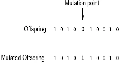
Mutation is applied to each child individually after crossover. It randomly alters each gene with a small probability (typically 0.001). Figure 3 shows the fifth gene of the chromosome being mutated. The traditional view is that crossover is the more important of the two techniques for rapidly exploring a search space. Mutation provides a small amount of random search, and helps ensure that no point in the search
Figure 3. A single Mutation
E. Convergence
The fitness of the best and the average individual in each generation increases towards a global optimum. Convergence is the progression towards increasing uniformity. A gene is said to have converged when 95% of the population share the same value. The population is said to have converged when all of the genes have converged. As the population converges, the average fitness will approach that of the best individual. A GA will always be subject to stochastic errors. One such problem is that of genetic drift. Even in the absence of any selection pressure (i.e. a constant fitness function), members of the population will still converge to some point in the solution space.
F. Termination
[image:2.612.330.540.392.506.2](a] A solution is found that satisfies minimum criteria Fixed number of generations reached
(b) Allocated budget (computation time/money) reached.
(c) The highest ranking solution's fitness is reaching or has Reached a plateau such that successive iterations no Longer produce better results
(d) Manual inspection (e) Combinations of the above.
G. Pseudo Code
Simple generational genetic algorithm pseudo code [a] Choose the initial population of individuals
[b] Evaluate the fitness of each individual in that population
[c] Repeat on this generation until termination: (time limit, sufficient fitness achieved, etc.)
[i] Select the best-fit individuals for reproduction. [ii] Breed new individuals through crossover and mutation
operations to give birth to offspring .
[iii] Evaluate the individual fitness of new individuals. [iv] Replace least-fit population with new individuals.
H. The Building Block Hypothesis
Genetic algorithms are simple to implement, but their behavior is difficult to understand. In particular it is difficult to understand why these algorithms frequently succeed at generating solutions of high fitness when applied to practical problems. The building block hypothesis (BBH) consists of:
[a] A description of a heuristic that performs adaptation by identifying and recombining "building blocks", i.e. low
order, low defining-length schemata with above average fitness.
[b] A hypothesis that a genetic algorithm performs adaptation by implicitly and efficiently implementing this heuristic.
Goldberg describes the heuristic as follows: "Short, low order, and highly fit schemata are sampled, recombined [crossed over], and resampled to form strings of potentially higher fitness. In a way, by working with these particular schemata [the building blocks], we have reduced the complexity of our problem; instead of building high-performance strings by trying every conceivable combination, we construct better and better strings from the best partial solutions of past samplings.
"Because highly fit schemata of low defining length and low order play such an important role in the action of genetic algorithms, we have already given them a special name: building blocks. Just as a child creates magnificent fortresses through the arrangement of simple blocks of wood, so does a genetic algorithm seek near optimal performance through the juxtaposition of short, low-order, high-performance schemata, or building blocks[6]
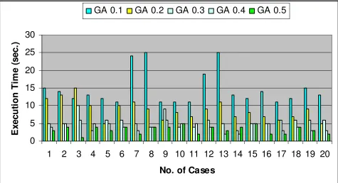
III. EXPERIMENT DESCRIPTION
First we generate the random population of individual .in this paper we consider the process scheduling problem .we have five jobs with their corresponding service time.
The parameter setting include inversion probability is .001and cross over probability is changed from 0.1 to 1.0. Then we compare the results of GA with variable cross over probability.
0
5
10
15
20
25
30
1
2
3
4
5
6
7
8
9 10 11 12 13 14 15 16 17 18 19 20
No. of Cases
E
x
e
c
u
ti
o
n
T
im
e
(
s
e
c
.)
[image:3.612.68.543.420.678.2]GA 0.1
GA 0.2
GA 0.3
GA 0.4
GA 0.5
Table 1. GA with CP (P=0.1 TO 0.5)
Sr.No Burst Time of Jobs GAc0.1 GAc0.2 GAc0.3 GAc0.4 GAc0.5
J1 J2 J3 J4 J5 Execution time in sec.
Execution time in sec.
Execution time in sec.
Execution time in sec.
Execution time in sec.
1 6 3 4 10 10 15 12 5 4 3
2 20 6 11 13 14 14 13 5 5 4
3 15 7 18 19 20 12 15 10 6 1
4 13 9 22 41 33 13 10 3 5 4
5 28 11 43 35 26 12 5 6 5 3
6 19 13 8 19 18 11 10 6 4 4
7 27 15 16 13 14 24 11 5 3 2
8 24 4 25 20 22 25 9 4 4 4
9 13 23 11 21 33 11 6 9 6 4
10 12 33 34 13 34 11 8 4 5 5
11 11 8 15 20 23 11 7 4 5 2
12 17 24 18 19 20 19 9 6 4 4
13 9 21 13 14 16 25 11 5 2 3
14 8 19 20 11 22 13 7 3 2 4
15 1 23 18 9 10 12 8 5 5 5
16 16 14 15 16 8 14 7 5 5 2
17 17 19 25 16 27 11 6 6 3 2
18 6 33 14 25 16 12 7 6 4 4
19 7 18 19 20 21 15 9 6 3 3
20 20 8 20 11 15 13 5 6 3 2
TOTAL E _ TIME
s= s=
1 20 = ES
293 175 109 83 65
MEAN E_ TIME
s= s=
1 2 0
=
ES
20
14.65 8.75 5.45 4.15 3.25
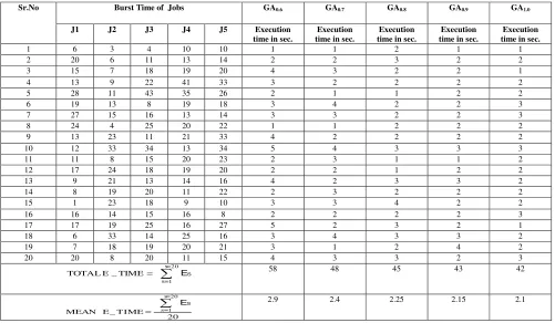
Table 2. GA with CP (P=0.5 TO 0.6)
Sr.No Burst Time of Jobs GA0.6 GA0.7 GA0.8 GA0.9 GA1.0
J1 J2 J3 J4 J5 Execution time in sec.
Execution time in sec.
Execution time in sec.
Execution time in sec.
Execution time in sec.
1 6 3 4 10 10 1 1 2 1 1
2 20 6 11 13 14 2 2 3 2 2
3 15 7 18 19 20 4 3 2 2 1
4 13 9 22 41 33 3 2 2 2 2
5 28 11 43 35 26 2 1 1 2 2
6 19 13 8 19 18 3 4 2 2 3
7 27 15 16 13 14 3 3 2 2 3
8 24 4 25 20 22 1 1 2 2 2
9 13 23 11 21 33 4 2 2 2 2
10 12 33 34 13 34 5 4 3 3 3
11 11 8 15 20 23 2 3 1 1 2
12 17 24 18 19 20 2 2 1 2 2
13 9 21 13 14 16 4 2 3 3 2
14 8 19 20 11 22 2 3 2 2 2
15 1 23 18 9 10 3 3 4 2 2
16 16 14 15 16 8 2 2 2 2 3
17 17 19 25 16 27 5 2 3 2 1
18 6 33 14 25 16 3 4 3 3 2
19 7 18 19 20 21 3 1 2 4 2
20 20 8 20 11 15 4 3 3 2 3
TOTAL E _ TIME
s= s=
1 20
= ES
58 48 45 43 42
MEAN E_ TIME
s= s=
1 2 0
=
ES
20
[image:4.612.54.555.425.717.2]IV. CONCLUSION AND FUTURE WORK
The Genetic algorithm is robust, flexible search method to optimize the scheduling problem. We examine that when the probability of crossover increase the execution time for job scheduling is decrease. i.e the GA converge to nearest optimal solution. Also the diversity of the Population increase .we can expand this work with variable mutation probability. The efficient parameter setting is required for the GA.
V. REFERENCES
[1] J.H. Holland. Adaptation in Natural and Artificial Systems. MIT Press, 1975.
[2] L. Davis. Genetic Algorithms and Simulated Annealing. Pitman, 1987.
[3] L. Davis. Handbook of Genetic Algorithms. Van Nostrand Reinhold, 1991.
[4] J.J. Grefenstette. Optimization of control parameters for genetic algorithms. IEEE Trans SMC, 16:122{128, 1986.
[5] J.J. Grefenstette. Genetic algorithms and their applications. In A. Kent and J.G. Williams, editors, Encyclopaedia of Computer Science and Technology, pages 139{152. Marcel Dekker, 1990.
[6] Goldberg, David E. (1989). Genetic Algorithms in Search Optimization and Machine Learning. Addison Wesley. pp. 41.
0
1
2
3
4
5
6
1
2
3
4
5
6
7
8
9
10 11 12 13 14 15 16 17 18 19 20
No.of Cases
E
x
e
c
u
ti
o
n
T
im
e
(S
e
c
.)