R E S E A R C H A R T I C L E
Open Access
A DAG-based comparison of
interventional effect underestimation between
composite endpoint and multi-state analysis in
cardiovascular trials
Antje Jahn-Eimermacher
1*, Katharina Ingel
1, Stella Preussler
1, Antoni Bayes-Genis
2and Harald Binder
1,3Abstract
Background: Composite endpoints comprising hospital admissions and death are the primary outcome in many cardiovascular clinical trials. For statistical analysis, a Cox proportional hazards model for the time to first event is commonly applied. There is an ongoing debate on whether multiple episodes per individual should be incorporated into the primary analysis. While the advantages in terms of power are readily apparent, potential biases have been mostly overlooked so far.
Methods: Motivated by a randomized controlled clinical trial in heart failure patients, we use directed acyclic graphs (DAG) to investigate potential sources of bias in treatment effect estimates, depending on whether only the first or multiple episodes are considered. The biases first are explained in simplified examples and then more thoroughly investigated in simulation studies that mimic realistic patterns.
Results: Particularly the Cox model is prone to potentially severeselection biasanddirect effect bias, resulting in underestimation when restricting the analysis to first events. We find that both kinds of bias can simultaneously be reduced by adequately incorporating recurrent events into the analysis model. Correspondingly, we point out appropriate proportional hazards-based multi-state models for decreasing bias and increasing power when analyzing multiple-episode composite endpoints in randomized clinical trials.
Conclusions: Incorporating multiple episodes per individual into the primary analysis can reduce the bias of a treatment’s total effect estimate. Our findings will help to move beyond the paradigm of considering first events only for approaches that use more information from the trial and augment interpretability, as has been called for in cardiovascular research.
Keywords: Composite endpoint, Recurrent events, Multi-state models, Hospital admissions, Bias, Cardiovascular
Background
When analyzing composite endpoints that incorporate an endpoint with multiple episodes, such as hospital admis-sion, a time to first event approach is frequently adopted for randomized clinical trials. Researchers from differ-ent disciplines have called for more appropriate methods of statistical analysis to more closely reflect the patients’
*Correspondence: [email protected]
1Institute of Medical Biostatistics, Epidemiology and Informatics, University Medical Center Johannes Gutenberg-University Mainz, Obere Zahlbacher Str. 69, 55131 Mainz, Germany
Full list of author information is available at the end of the article
disease burden. This involves a discussion on whether multiple episodes per patient are to be analyzed. So far, this discussion mostly has considered power issues, while overlooking potential bias. In this work, we investigate sources of bias and show that there can be a poten-tially severe underestimation of treatment effect esti-mates, when derived only based on first events, that can be substantially reduced by adequately modeling multiple episodes per patient.
Composite endpoints combine several events of inter-est into a single variable, usually defined as a time to event
outcome. They are frequently used as primary or sec-ondary endpoints in cardiovascular clinical trials [1, 2]. Composite outcomes facilitate the evaluation of treatment effects when unrealistically large sample sizes would be required to detect differences in the incidence of single outcomes among treatment groups, for example mor-tality. While using a composite outcome may help in terms of power, at the same time it introduces its own difficulties concerning interpretation of trial results and methodological challenges [2–6]. One major concern is that endpoints occurring in individual patients usually are clinically related (such as nonfatal and fatal myocar-dial infarctions). Multi-state modeling of these relations by allowing for separate transition hazards between the different subsequent events has recently been proposed for large cardiovascular observational studies [7, 8]. How-ever, for randomized clinical trials this is suspected to attenuate the power and confirmatory character of the trial [9]. In the majority of clinical trials, the concern for potential relations between clinical episodes is there-fore addressed by counting only one event per patient and analyzing the time to the first of all components. By following this approach, only data on the first episode per individual are used for the primary statistical anal-ysis, even when subsequent episodes (including deaths) have been recorded. There is an ongoing debate, in par-ticular in cardiovascular research, on the efficiency and validity of this practice because it ignores a great deal of clinically relevant information [3, 10–12]. The impact of multiple episodes per patient on the power of a clinical trial is apparently promising [3, 13], and selected statisti-cal methods have been exemplarily applied to single trial data [14–16]. However, less attention is paid to the esti-mation and interpretability of treatment effects that can be substantially attenuated depending on whether multi-ple episodes are analyzed or not. We consider this critical since the choice of a statistical method for analyzing trial data should not be mainly driven by power consider-ations but by the objective to obtain an unbiased and meaningful treatment effect estimate, i.e. to make causal inferences about the treatment and its (added) benefit and to understand how a treatment influences a patient’s disease burden.
Although randomized clinical trials are often suspected to produce unbiased results as the randomized treatment allocation prevents confounding, hazard-based survival analysis can introduce its own bias [17–20]. In particu-lar, the Andersen-Gill approach [21] has been suspected to introduce bias by erroneously modeling that a clini-cal episode will leave a patient’s risk profile unchanged and will not affect the incidence rate for future episodes [22–25]. This finding has been controversially discussed as it implicitly assumes that direct effects are to be esti-mated [26]. The causal directed acyclic graphs approach
(DAG) [27, 28] has been proposed for defining adequate statistical models that prevent or minimize bias in the presence of confounding. It is a powerful tool for iden-tifying and addressing bias and is increasingly popular, but it is primarily applied in epidemiological research. In this work, we will make use of this approach for randomized clinical trials to provide an accessible expla-nation of potential bias in proportional hazards-based survival analysis of first and multiple episodes of a com-posite endpoint and to define adequate statistical models for reducing or preventing bias. While the use of DAGs may be problematic in a continuous time setting [29], we are avoiding such issues by first considering actual dis-crete states in DAG analysis, and making the transition to continuous time settings with evidence from simulations. The article is organized as follows: We motivate this research with a clinical example in “Cardiovascular clinical trial example” section. Then, in “Methods” section, we first formalize potential bias via directed acyclic graphs and illustrate the findings on simplified examples. There-after we identify statistical models that have the potential to reduce that bias. We support our findings by simulation studies that mimic the motivating clinical trial situation and present the results in “Results” section. Finally, we finish the article with a discussion in “Discussion” section.
Cardiovascular clinical trial example
to first composite endpoint is analyzed, a total number of
N =465 patients is required to attain a power of 80% for rejecting the null hypothesis of no treatment effect on the incidence of the composite endpointH0= {HR=1}[30]. Incorporating recurrent events into the statistical analysis has the potential to decrease the sample size to up toN=
223 [13], and thus is apparently promising for improving the feasibility and efficiency of the trial. However, disease-associated complications that require a hospital admission will obviously affect the risk for further non-fatal and fatal outcomes. For example, patients who acquire a non-fatal MI have an increased risk for fatal and non-fatal outcomes thereafter. Concern arises if this might question the study results, and, more generally, how incorporating recurrent events into the primary statistical analysis will affect the treatment effect estimates and thus the interpretation of trial results.
Methods
Formalizing potential bias via directed acyclic graphs The graphical representation of causal effects between variables [27, 28] helps to understand the sources of potential bias when estimating some causal effect of an exposure to an outcome and how different statistical mod-els differently address that bias. In the causal directed acyclic graph (DAG) approach, an arrow connecting two variables indicates causation; variables with no direct causal association are left unconnected. We will use this approach for illustrating the causal system in randomized clinical trials when a composite endpoint is investigated that comprises fatal and non-fatal events. An example is the composite of cardiovascular death and hospital admission for heart failure disease as defined in the moti-vating clinical trial example (“Cardiovascular clinical trial example” section). Effect estimation is assumed to be hazard-based with a proportional hazards assumption.
Selection bias
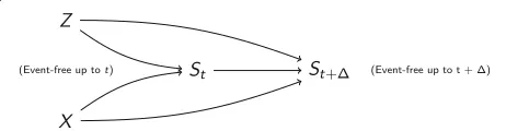
Figure 1 illustrates the causal system in a time to first composite endpoint approach. The randomized treatment (X) is the exposure variable, that is assumed to affect the fatal and non-fatal outcomes and thus the composite end-point. In addition to treatment, further disease or patient
Fig. 1Directed acyclic graph for the causal system between treatment (X), being free of any event at timet(St) andt+(St+), and unobserved variables (Z) that are unrelated to treatment (for example by randomization) and affect the event rate. Figure according to Aalen et al. [20]
characteristics will affect the risk for adverse outcomes. Some are known, others are unknown or unmeasurable (summarized as a single unobserved variable Z). Obvi-ously, being free of any event at timet(St) is a collider on
the path between the exposure treatment and the unob-served variable Z. Conditioning on a collider will open the path between the variables that are connected by the col-lider and thus artificially introduce spurious associations [31]. Each contribution to the partial likelihood in the Cox proportional hazards model is a conditional contribution, conditional on being free of any event up to that time. Therefore, an association is induced between the actu-ally unrelated randomized treatment and the unobserved variable Z. As Z affects the outcomes, this association will bias the treatment’s effect estimate for the fatal, non-fatal and composite outcome. This bias is calledselection bias and has been investigated for incidence rate ratios [28] and hazard ratios [17, 18, 20, 32] before. We will illustrate selection bias by a simple example at the end of this subsection. Whereas conditioning on being alive is an unavoidable step in the hazard-based analysis, we can pre-vent conditioning on being free of any epre-vent by including the recurrent non-fatal events into the statistical model: the at-risk set in the partial likelihood estimator then com-prises all subjects that are still alive in contrast to a set of those subjects only that are free of any event at the partic-ular time point. This way, incorporating recurrent events will reduce selection bias when estimating the treatment effect on the fatal and non-fatal outcomes and will thus also reduce the bias when estimating the treatment effect on the composite endpoint. In summary, the first insight gained from a formalization via DAGs is that analyzing all non-fatal events, also the recurrent ones, in the statistical model for the composite endpoint will reduce selection bias.
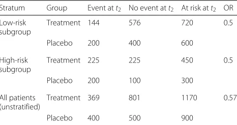
within each subgroup and for each timet1andt2 (con-stant hazard ratio assumption). From the odds ratio and the expected failure rates per subgroup in the control group att1, we can derive the expected failure rates att1 for the treatment group, which are 1/5 and 1/2, respec-tively. For the example of a sample size ofN = 1800 per treatment group, Table 1 shows the number of event-free subjects just beforet2per treatment group and subgroup and the expected number of failures att2as derived from the expected failure rates of 1/3 and 2/3 in the control group and 1/5 and 1/2 in the treatment group. Whereas the odds ratio is unbiased when estimated within each subgroup (0.5), the crude odds ratio estimated from the marginal table is 0.57, indicating a smaller treatment effect (selection bias) that is obtained when conditioning on being event-free but not takingZinto account. As indi-cated, Z might be unobserved, making conditioning on
Z problematic. The selection bias does not depend on sample size, which was chosen to be large in this data example to obtain integer patient numbers. The difference between conditional and unconditional modeling remains when moving from discrete time to continuous time, i.e. when the interval between two potential failures becomes infinitesimally small and the hazard ratio is defined on a continuous time scale. Simulation results (“Simulation studies” section) will further support this finding.
Direct effect bias
When following the recommendation to include recur-rent events into the statistical model as derived from the previous section, concern might arise as to how to model the transitions from one non-fatal event to a succeeding fatal or non-fatal event. From cardiovascular research it is well known that the different components in a composite endpoint are related. For example, a non-fatal myocar-dial infarction will apparently affect the risk for further fatal or non-fatal cardiovascular outcomes. To address
Table 1Expected patient numbers in the discrete failure time example for time to first event stratified by subgroup (“Selection bias” section)
Stratum Group Event att2 No event att2 At risk att2 OR
Low-risk subgroup
Treatment 144 576 720 0.5
Placebo 200 400 600
High-risk subgroup
Treatment 225 225 450 0.5
Placebo 200 100 300
All patients (unstratified)
Treatment 369 801 1170 0.57
Placebo 400 500 900
Patients are at risk for a first event att2, if they have not experienced an event att1.
Odds Ratio (OR) for experiencing an event under treatment as compared to control
this concern, we will again apply the approach of directed acyclic graphs. Figure 2 illustrates the causal system when more than only the first event is considered and the risk for further events is potentially changing with each non-fatal event. The number of events experienced until time
t, N(t), is a mediator lying along the causal pathway between treatmentXand the number of events att+,
N(t + ). Conditioning on or stratifying by the num-ber of previously experienced events will close this path, and the treatment effect estimate is reduced to the treat-ments’ direct effect on the outcome, whereas its indirect effect is not considered. While direct effects are interest-ing from a biological viewpoint, estimation of total effects is important from the clinical, health care, and patients’ perspective. For example, the mortality rate increases after a non-fatal myocardial infarction, and therefore a treat-ment that effectively prevents myocardial infarctions in general reduces the mortality (indirect effect), besides its direct effect on mortality. Both, direct and indirect effects, define a treatment’s total effect. We will illustrate the dif-ference between direct and total effect estimation in a simple example at the end of this section. In summary, the second insight gained from a formalization via DAGs is to not condition on the individual’s event history by stratifying or adjusting for the previous non-fatal events for estimating a treatments total effect. In contrast, in a time to first event analysis, the effect estimate is natu-rally restricted to the direct effect as it is derived only from those pathways, that start from the exposure variable treatment. We use the termdirect effect biaswhen effect estimates are reduced to direct effects only.
Example Again, consider a balanced randomized trial comparing the time to event under a particular treatment as compared to some control intervention. As before, we consider a setting with discrete times, that can be trans-ferred to the continuous time Cox proportional hazards model. We assume that non-fatal events are experienced at time t1and can be followed by death at timet2. The risk for experiencing a non-fatal event at t1 is assumed to be 2/3 in the control group and 1/3 in the treament group, respectively. The mortality rate in patients who have acquired the non-fatal event att1increases to 40% as compared to a 20% risk in those subjects who are free of an event att1. Mortality rates are assumed to be not affected by treatment conditionally on the number of prior events,
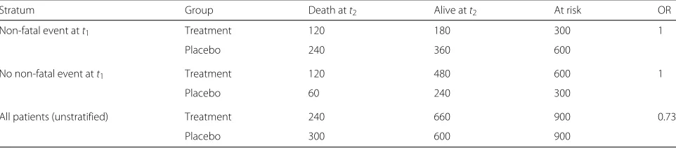
i.e. neither before nor after having experienced a non-fatal event. For the example of a total sample size ofN=1800, Table 2 shows the expected number of death cases strat-ified by having experienced a preceding non-fatal event at t1 and marginally over all subjects. Whereas within each stratum no treatment effect on mortality is observed, respectively, the odds ratio estimated from the marginal table is 0.73, indicating a positive treatment effect on mortality. This result indicates that treatment effectively reduces mortality by preventing subjects from entering that stratum, which is characterized by a higher mortality rate (total effect), although it has no direct effect on the mortality rates at all. Effect estimates differ when condi-tioning on prior events or not, irrespective of sample size, and when moving from discrete time to continuous time, thus when deriving the hazard ratio in a continuous time scale. Simulation results (“Simulation studies” section) will further support this finding.
Reducing bias by statistical modeling
We will now transfer the insights on biased effect esti-mation as derived from the DAGs to identify statistical analysis models that have the potential to reduce that bias. Consider a randomized clinical trial withnsubjects fol-lowed for a composite endpoint. Subjects will be indexed by i, events by j. Let TCE∗ ,ij be a series of random vari-ables that describe the time from starting point 0 to the
j-th occurrence of the composite endpoint in subjecti. Let furtherCibe independent identically distributed random
variables that describe the time to censoring. We observe
TCE,ij = min(TCE∗ ,ij,Ci), the time to composite endpoint
or censoring, whichever comes first, and the indicator variablesδij=I
TCE∗ ,ij≤Ci
.
It has been proposed to describe the distribution of
TCE,ij by a multiplicative intensity process [34], Yi(t) ·
λCE,i(t), of the underlying counting process
Ni(t):=#
j; TCE,ij≤t ∧ TCE∗ ,ij≤Ci
,
with deterministic hazard function λCE,i(t) (Fig. 3) and
Yi(t) = I{t ≤ Ci}. Figure 3 sketches a model that
comprises all events, also the recurrent ones (CE1,
CE2. . . ), without conditioning on or stratifying by the event history (transition hazards between the succeed-ing events do not change). If conditional on covariates λCE,ihas a Cox proportional hazards shape, this model is
known as the Andersen-Gill [21] model.
λCE(t|Xi)=λCE,0(t)·exp(βXi) (1)
withXi being thep-dimensional vector of covariates for
subject i and β being the vector of regression coeffi-cients. The Andersen-Gill model was recently applied to re-analyze clinical trials in patients suffering from heart failure to evaluate the effect of new therapies on the patients risk of the composite of hospitalizations due to heart failure and cardiovascular death [14–16]. The treat-ment effectβis then estimated by maximizing the partial likelihood
PLAG(β) =
i
j ⎛
⎝ exp(βXi) k∈RAG(ij)exp(βX
k)
⎞ ⎠
δij
(2)
The at-risk setRAG(ij) includes all subjects who have not been censored and have not died before timetij, the time
when individuali experiences itsj-th event. In contrast, in a stratified model as proposed by Prentice et al. [35], the at-risk set RPWP(ij) is restricted to only those subjects who are at risk for experiencing thej-th event at timetij,
thus having experiencedj−1 events before. However, fol-lowing the arguments of “Formalizing potential bias via directed acyclic graphs” section, the Andersen-Gill model allows the estimation of total effects by not stratifying on the event history, in contrast to the stratified model that is estimating direct effects only [26]. Both models are still susceptible to selection bias as they naturally restrict the risk sets to subjects being alive. However, they reduce the selection bias as compared to results derived from a Cox proportional hazards model with partial likelihood
Table 2Expected patient numbers in the discrete failure time example for time to death stratified by previously experienced non-fatal event (“Direct effect bias”section)
Stratum Group Death att2 Alive att2 At risk OR
Non-fatal event att1 Treatment 120 180 300 1
Placebo 240 360 600
No non-fatal event att1 Treatment 120 480 600 1
Placebo 60 240 300
All patients (unstratified) Treatment 240 660 900 0.73
Placebo 300 600 900
Fig. 3Unstratified transition hazard model for the transitions between study start (S) and the recurrent composite endpoints (CE1,CE2. . . )
PLC(β) =
i ⎛
⎝ exp(βXi) k∈RC
(i)exp(βX
k)
⎞ ⎠
δi1
(3)
as in this model the risk setsRC(i)are restricted to subjects that are not only still alive but also free of any previous non-fatal event at timeti1, the time of the first event or censoring of individuali.
The partial likelihood (2) of the unstratified maximally unrestricted Andersen-Gill model (1) can be re-written as
PLAG(β) =
l
i
jl ⎛
⎝ exp(βXi) k∈RAG(
ijl)exp(βX
k)
⎞ ⎠
δijl
(4)
with l = 1,. . .,L indexing the L components of the composite and jl indexing the events of type l and δijl
again being the corresponding event indicator. Therefore, model (2) can also be described as a multi-state model that allows for different baseline transition hazards for the dif-ferent components. Figure 4 sketches this model for the motivating example of two components: death (D) and hospital admission (H1,H2. . .) with
λl(t|Xi) = λl,0(t)exp(βXi),l=1, 2. (5)
By defining a single vector β for both the transition hazards λ1 andλ2, a constraint is induced, namely that the covariates equally affect fatal and non-fatal events. In particular, for our motivating example this means that treatment has the same effect on the fatal and non-fatal outcomes. This constraint has in fact been described as a requirement for the proper use of composite endpoints, for example by regulatory agencies [36]. However, at the same time it has been observed that in practice this assumption is frequently violated. Ferreira-Gonzalez et al. [37] conclude from a systematic literature review that effects of treatments in cardiovascular clinical trials differ
strongly between the components, with larger effects in less relevant components and the smallest effects in mor-tality. The same has been observed in several clinical trials on heart failure disease [14, 16]. To relax the constraint of a common treatment effect on all components, the more general multi-state model (MS) can be defined by transition hazards
λl(t|Xi) = λl,0(t)exp(βlXi),l=1. . .L (6)
and partial likelihood
PLMS(β1,. . .,βL)=
l
i
jl ⎛
⎝ exp(βlXi) k∈RMS
(ijl)exp(βlX
k)
⎞ ⎠
δijl
. (7)
and risk sets RMS(ij
l) that include all subjects who have
not been censored and have not died before the par-ticular event time, respectively. This generalization of the Andersen-Gill model allowing for separate treatment effects for each component, βl, can be proposed
when-ever sample size and event frequency allow for such an approach. It still does not stratify on the event history and does not restrict the at-risk-set only to those subjects that are free of any event, but allows for a higher flexibility with respect to differential treatment effects.
Note, that we focus on marginal models within this manuscript. By introducing a (joint) frailty term into model (5) or (6) and applying penalized likelihoods [38], a conditional joint frailty model could also be fitted. By conditioning on the frailty term the selection bias as illustrated in Fig. 1 is minimized, however at the price of increasing the model complexity by introducing fur-ther model assumptions (joint frailty distribution) and parameters (frailty variance). We will show in the next section that in many applications one can safely stay with the marginal model, thereby following theOccam’s razor principle.
Simulation studies
We investigate the bias in treatment effect estimation as identified in “Formalizing potential bias via directed acyclic graphs” section (selection bias, direct effect bias) in simulation studies. The simulation study mimics the clini-cal trial situation that has motivated this research. For this
purpose, we consider a balanced randomized clinical trial with a follow-up of two years and uniformly distributed recruitment ofN = 380 individuals over the first year. The transition hazardsλ1 andλ2(Fig. 4 and Eq. (6)) for the transitions to fatal and non-fatal events, respectively, are defined byλl(t|Xi)=λl·exp(βlXi).
Baseline annual death and admission rates are defined asλ1 = 0.14 andλ2 = 1.17, respectively. Further sim-ulations are performed where fatal and non-fatal events equally contribute to the same overall annual event rate, thusλ1 = λ2 = 0.655. Treatment is assumed to equally affect both components of the composite, and we define β = β1 = β2 = log(0.75) as was expected in the planning phase of the STRONG-HF trial. We addition-ally consider situations where treatment has a minor effect on mortality (β1 = log(0.92)), following the findings of a systematic literature review on cardiovascular clinical trials [37]. To consider that unobserved or unmeasurable variables affect the outcomes, we define an unobserved variableZiper individuali. TheZiare generated as
inde-pendent and gamma-distributed random variables with mean 1 and varianceθ. Following a frailty approach,Ziis
assumed to act multiplicatively on the hazard by
λl(t|Xi,Zi) = λl,0(t)·Zi·exp(βlXi),l=1, 2 (8)
Note that the unobserved variable acts on both tran-sition hazards, inducing a correlation between both pro-cesses. Such a joint model [38] is considered to more closely mimic real clinical trial data as compared to simulation models assuming independency between the event processes, as in most situations it can be expected that patient and disease characteristics will affect adverse disease outcomes towards the same direction. Different θ ∈ {0, 0.2,. . ., 1}reflect different strengths of association between the unobserved variable and the fatal and non-fatal outcomes and will therefore cause different degrees of selection bias. In a second simulation study we add an indirect effect of treatment on the composite outcome by defining the transition hazards to be increasing by a factor ofρwith each non-fatal event. By applying a range of val-ues betweenρ = 1 (no increase of hazards) andρ = 1.3 (increase of hazards by 30% with each non-fatal event), different degrees of the indirect effects are evaluated.
In a third simulation study we investigate treatment effect estimation when both effects are present, that is the transition hazards increase with each non-fatal events by a factor of ρ (ρ ∈ [1, 1.3]) while in addition a gamma-distributed frailty term with mean 1 and a moderate variance ofθ =0.6 acts on all transition hazards. For each simulation model 5000 datasets are simulated, respec-tively.
All simulated data are analyzed by the Andersen-Gill model for the composite endpoint (1) and its multi-state extension (6) to estimate separate treatment effects on
fatal and non-fatal outcomes. Both models are applied to the full simulated datasets and to datasets that are restricted to the first composite endpoint per individ-ual. For the restricted data, the Andersen-Gill model then reduces to a Cox proportional hazards model and its multi-state extension to a competing risk model.
All data are simulated and analyzed in the open-source statistical environmentR, version 3.1.0 (2014-04-10) [39] and by extending the published simulation algorithm for recurrent event data [40]. Mean regression coefficient estimates are derived together with standard errors as estimated from their variability among the simulations.
Results
Simulation results are presented in Tables 3 and 4 for λ1 ∈ {0.14, 0.655}, β1 ∈ {log(0.92), log(0.75)}, ρ ∈
Table 3 Simulation results for λ1 = 0.14 and λ2 = 1.17 Simulation p arameters Results of 1st-event-analyses Results of all-events-analyses exp (β1 ) exp (β2 )θ ρ exp (
β)CE SE(β
CE
)
exp
(
β)1 SE(β
1
)
exp
(
β)2 SE(β
2
)
exp
(
β)CE SE(β
CE
)
exp
(
β)1 SE(β
1
)
exp
(
Table 4 Simulation results for λ1 = 0.655 and λ2 = 0.655 Simulation p arameters Results of 1st-event-analyses Results of all-events-analyses exp (β1 ) exp (β2 )θ ρ exp (
β)CE SE(β
CE
)
exp
(
β)1 SE(β
1
)
exp
(
β)2 SE(β
2
)
exp
(
β)CE SE(β
CE
)
exp
(
β)1 SE(β
1
)
exp
(
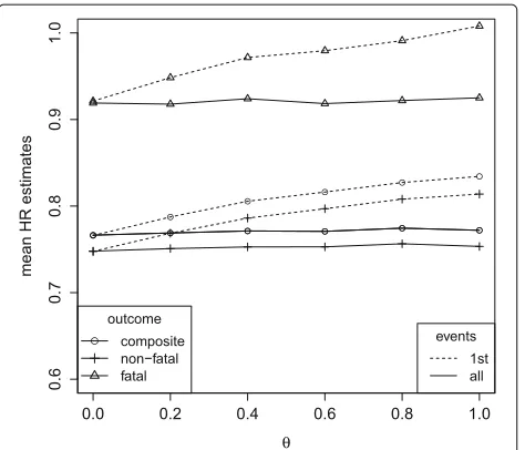
Fig. 5Mean hazard ratio estimates in the simulation model under
λ1=0.14,λ2=1.17,ρ=1, a common treatment effect on non-fatal and fatal outcomes (β1=β2=log(0.75)) and varying influence of an unobserved variableZ(having varianceθ). Cox proportional hazards analysis for the composite and the single components, respectively (1st events), Andersen-Gill analysis (all events, composite outcome) and multi-state analysis (all events, fatal and non-fatal outcomes)
Fig. 6Mean hazard ratio estimates in the simulation model under
λ1=0.14,λ2=1.17,ρ=1, a lower treatment effect on fatal than on non-fatal outcomes (log(0.92)=β1> β2=log(0.75)) and varying influence of an unobserved variableZ(having varianceθ). Cox proportional hazards analysis for the composite and the single components, respectively (1st events), Andersen-Gill analysis (all events, composite outcome) and multi-state analysis (all events, fatal and non-fatal outcomes)
differ by outcome. However, compared to the setting with a common treatment effect (Fig. 5), all effect estimates are similarly affected by selection bias with respect to the direction and magnitude of that bias.
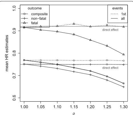
Figure 7 shows the simulation results for data ran-domly generated under transition hazards for fatal and non-fatal events that are equally affected by treatment and increase by a factor ofρ with each non-fatal event. No unobserved variable is introduced in this simula-tion model to clearly differentiate between the different sources of bias. Whereas direct and total effects coincide when transition hazards remain unaffected by previous events (ρ = 1), Fig. 7 clearly shows that direct and total effects substantially differ when transition hazards increase with non-fatal events (ρ >1). The analysis of 1st events provides direct effect estimates whereas the anal-ysis of all events provides total effect estimates according to the findings of “Formalizing potential bias via directed acyclic graphs” section. By preventing experiencing a first non-fatal event, the treatment prevents the patients from becoming at an increased risk for further events. This con-tributes to the indirect effect, and thus to a larger total treatment effect as compared to its direct effect. Under an increased mortality rate (λ1 = 0.655), the process for recurrent events stops earlier on average due to the higher frequency of competing terminal events. Thus, the indi-rect effect of the treatment (preventing later events that occur with an increased risk rate), contributes less to the
Fig. 7Mean hazard ratio estimates in the simulation model under
total effect estimates. Therefore, differences between total and direct effect estimates become smaller: whereas under λ1 = 0.14,θ = 0 andρ = 1.3 the total effect in terms of the hazard ratio is estimated as 0.65 as compared to the direct effect of 0.75 (Table 3), underλ1 = 0.655 the total effect estimate of 0.72 is more closely approaching the direct effect (Table 4).
Again, when treatment differentially affects the risk for fatal and non-fatal outcomes (Fig. 8), direct and total effect estimates also differ for each single outcome. The direction and magnitude of these differences are compara-ble to the results observed for common treatment effects (Fig. 7).
As the hazard for the composite endpoint is the sum of the hazards over the two components [41], the hazard ratio can be derived as 1/(λ1+λ2)i2=1λiexp(βi)in the
situation of constant hazards. This weighted sum is esti-mated when analysing the composite outcome using first events only or all events as long as no selection bias and no indirect effects are present, that isθ =0 for the anal-ysis of 1st events andρ = 1 for the analysis of all events (Figs. 6 and 8).θ > 0 and/orρ > 1 then affect the esti-mates for the composite endpoint in the same direction as the estimates for the single components.
Whereas selection bias is attenuating the treatment effect estimates, hazards that increase with each non-fatal event induce the total effect estimates to become larger than the direct effect only. As a consequence, the
Fig. 8Mean hazard ratio estimates in the simulation model under
λ1=0.14,λ2=1.17,θ=0, a lower direct treatment effect on fatal than on non-fatal outcomes (log(0.92)=β1> β2=log(0.75)) and transition hazards that increase by a factor ofρafter each non-fatal event. Cox proportional hazards analysis for the composite and the single components, respectively (1st events), Andersen-Gill analysis (all events, composite outcome) and multi-state analysis (all events, fatal and non-fatal outcomes)
differences between direct and total treatment effect esti-mates decrease with increasing degree of selection bias. Whereas exp(βˆ2)decreased from 0.75 to 0.65 when haz-ards increase by 0 to 30% with each non-fatal event, under θ = 0.6 only a decrease up to 0.72 is still observed (Table 3). Under a higher mortality rate ofλ1=0.655 even not any decrease in the total effect estimate is observed (exp(βˆ2) = 0.78) as here the selection bias starts to prevail (Table 4).
Discussion
Potential biases in analysis of composite endpoints that comprise endpoints with multiple episodes, such as hos-pital admission, have been mostly overlooked so far. To advance the state-of-the-art, we provided an accessible explanation of biases in this setting, that is supported by simulation results. Our results show that the initial step in modeling must be defining the treatment effect that is of interest: A total treatment effect estimate can only be derived by analysing all events, whereas only the direct treatment effect can be estimated from analyses of 1st events or from analyses that are stratified by event his-tory. When interpreting trial results, eventually derived from different statistical models, one must be aware, that the direct effect estimates can be severly more prone to selection bias. Our findings will help to move beyond the paradigm of considering first events only for approaches that use more information from the trial and augment interpretability, as has been called for in cardiovascular research [11, 12].
The association of some variable with the outcome is not a reasonable criterion for covariate selection in mul-tiple regression, as has been described in epidemiology for example to explain the birth-weight paradox [42]. We use similar arguments in randomized clinical trials to jus-tify that adjusting or strajus-tifying for the patients’ disease history within trial time is inadequate for estimating a treatments’ total effect.
models [38, 44] to prevent from bias. However, their find-ings are based on simulation studies with high mortality rates (up to 31%), which explains these controversial con-clusions. Balan et al. [45] recently proposed a score test for deciding between multi-state and joint frailty mod-eling. All these findings confirm, that using composite endpoints in randomized clinical trials can not eliminate the bias arising from the association between the risk pro-cesses of the single components as long as only the first event is analyzed [46].
We have focused on the estimation of a treatment effect based on proportional hazards. Additive hazard models have been recommended instead as they are unaffected by non-collapsibility [20, 47].
Hazard ratios are used to assess the early benefit of new drugs compared to some control [48]. Our results indicate the need to further specify the estimand, the assessment refers to: a treatment’s direct or its total effect as both can differ substantially.
In recent years alternatives to hazard-based analyses of composite endpoints have been proposed based on weighted outcomes [49–51] to consider that not all com-ponents are of the same clinical relevance and importance for the patients. The multi-state approach proposed in this paper allows a separate investigation of treatment effects on the different components, and it seems to be important to compare both approaches with respect to interpretabil-ity of treatment effect estimation and power. Concern-ing power, the multi-state approach requires some kind of multiplicity adjustment as different treatment effects are estimated for the different components. Sequentially rejective test procedures provide a powerful and flexible tool to control type I error. As with other multivari-ate time to event outcomes, closed form solutions for sample size planning will be difficult to obtain [52], but simulation algorithms allow for an extensive investiga-tion of sample size requirements, including for complex models [40, 52].
Conclusion
This manuscript provides an accessible explanation of potential biases in treatment effect estimation when analysing composite endpoints. It illustrates that the risk for bias and its degree depend on whether first or multi-ple episodes per patient are analysed. Integrating multimulti-ple episodes into the statistical analysis model has the poten-tial to reduce selection bias and to additionally capture indirect treatment effects. In particular for cardiovascu-lar research, these findings may help to move beyond the paradigm of considering first events only.
Acknowledgements
We thank Daniela Zoeller and two referees for their constructive comments improving the manuscript and Kathy Taylor for proof-reading.
Funding
This research was supported by a grant of the Deutsche Forschungsgemeinschaft (DFG) grant number JA 1821/4.
Availability of data and materials
Not applicable.
Authors’ contributions
AJ developed the method, produced the results and wrote the first draft of the manuscript. KI derived the sample size requirements for the STRONG-HF trial and contributed to the methods. SP implemented the simulations. AB designed the STRONG-HF trial and contributed to the introduction, results and discussion sections. HB contributed to all parts of the manuscript. All authors read and approved the final manuscript.
Competing interests
The authors declare that they have no competing interests.
Consent for publication
Not applicable.
Ethics approval and consent to participate
Not applicable.
Publisher’s Note
Springer Nature remains neutral with regard to jurisdictional claims in published maps and institutional affiliations.
Author details
1Institute of Medical Biostatistics, Epidemiology and Informatics, University Medical Center Johannes Gutenberg-University Mainz, Obere Zahlbacher Str. 69, 55131 Mainz, Germany.2Heart Failure Clinic, Cardiology Service, CIBERCV, Department of Medicine, UAB, Hospital Universitari Germans Trias i Pujol, Carretera del Canyet, 08916 Badalona, Barcelona, Spain.3Institute for Medical Biometry and Statistics, Faculty of Medicine and Medical Center - University of Freiburg, Stefan-Meier-Str. 26, 79104 Freiburg, Germany.
Received: 10 November 2016 Accepted: 9 June 2017
References
1. Lim E, Brown A, Helmy A, Mussa S, Altman DG. Composite outcomes in cardiovascular research: a survey of randomized trials. Ann Intern Med. 2008;149(9):612–17.
2. Freemantle N, Calvert M, Wood J, Eastaugh J, Griffin C. Composite outcomes in randomized trials: greater precision but with greater uncertainty? JAMA. 2003;289(19):2554–9.
3. Ferreira-González I, Permanyer-Miralda G, Busse JW, Bryant DM, Montori VM, Alonso-Coello P, Walter SD, Guyatt GH. Methodologic discussions for using and interpreting composite endpoints are limited, but still identify major concerns. J Clin Epidemiol. 2007;60(7):651–7. 4. Freemantle N, Calvert M. Weighing the pros and cons for composite
outcomes in clinical trials. J Clin Epidemiol. 2007;60(7):658–9. 5. Montori VM, Permanyer-Miralda G, Ferreira-González I, Busse JW,
Pacheco-Huergo V, Bryant D, Alonso J, Akl EA, Domingo-Salvany A, Mills E, Wu P, Schünemann HJ, Jaeschke R, Guyatt GH. Validity of composite end points in clinical trials. BMJ. 2005;330(7491):594–6. 6. Chi GYH. Some issues with composite endpoints in clinical trials. Fundam
Clin Pharmacol. 2005;19(6):609–19.
7. Ieva F, Jackson CH, Sharples LD. Multi-state modelling of repeated hospitalisation and death in patients with heart failure: The use of large administrative databases in clinical epidemiology. Stat Methods Med Res. 2017;26(3):1350–72.
8. Ip EH, Efendi A, Molenberghs G, Bertoni AG. Comparison of risks of cardiovascular events in the elderly using standard survival analysis and multiple-events and recurrent-events methods. BMC Med Res Methodol. 2015;15(1):15.
10. Anker SD, Schroeder S, Atar D, Bax JJ, Ceconi C, Cowie MR, Crisp A, Dominjon F, Ford I, Ghofrani HA, Gropper S, Hindricks G, Hlatky MA, Holcomb R, Honarpour N, Jukema JW, Kim AM, Kunz M, Lefkowitz M, Le Floch C, Landmesser U, McDonagh TA, McMurray JJ, Merkely B, Packer M, Prasad K, Revkin J, Rosano GMC, Somaratne R, Stough WG, Voors AA, Ruschitzka F. Traditional and new composite endpoints in heart failure clinical trials: facilitating comprehensive efficacy assessments and improving trial efficiency. Eur J Heart Fail. 2016;18(5):482–89. 11. Anker SD, McMurray JJV. Time to move on from ‘time-to-first’: should all
events be included in the analysis of clinical trials? Eur Heart J. 2012;33(22):2764–5.
12. Claggett B, Wei LJ, Pfeffer MA. Moving beyond our comfort zone. Eur Heart J. 2013;34(12):869–71.
13. Ingel K, Jahn-Eimermacher A. Sample-size calculation and reestimation for a semiparametric analysis of recurrent event data taking robust standard errors into account. Biometrical J. 2014;56(4):631–48.
14. Rogers JK, McMurray JJV, Pocock SJ, Zannad F, Krum H, van Veldhuisen DJ, Swedberg K, Shi H, Vincent J, Pitt B. Eplerenone in patients with systolic heart failure and mild symptoms: analysis of repeat hospitalizations. Circulation. 2012;126(19):2317–23.
15. Rogers JK, Pocock SJ, McMurray JJV, Granger CB, Michelson EL, Östergren J, Pfeffer Ma, Solomon SD, Swedberg K, Yusuf S. Analysing recurrent hospitalizations in heart failure: a review of statistical methodology, with application to CHARM-Preserved. Eur J Heart Fail. 2014;16(1):33–40.
16. Rogers JK, Jhund PS, Perez AC, Böhm M, Cleland JG, Gullestad L, Kjekshus J, van Veldhuisen DJ, Wikstrand J, Wedel H, McMurray JJV, Pocock SJ. Effect of rosuvastatin on repeat heart failure hospitalizations: the CORONA Trial (Controlled Rosuvastatin Multinational Trial in Heart Failure). JACC Heart Fail. 2014;2(3):289–97.
17. Schmoor C, Schumacher M. Effects of covariate omission and categorization when analysing randomized trials with the Cox model. Stat Med. 1997;16(1-3):225–37.
18. Hernan MA. The Hazards of Hazard Ratios. Epidemiology. 2010;21(1):13–5. 19. Cécilia-Joseph E, Auvert B, Broët P, Moreau T. Influence of trial duration
on the bias of the estimated treatment effect in clinical trials when individual heterogeneity is ignored. Biom J. 2015;57(3):371–83. 20. Aalen OO, Cook RJ, Rysland K. Does Cox analysis of a randomized survival
study yield a causal treatment effect? Lifetime Data Anal. 2015;21(4): 579–93.
21. Andersen PK, Gill RD. Cox’s regression model for counting processes: a large sample study. Ann Stat. 1982;10(4):1100–20.
22. Jahn-Eimermacher A. Comparison of the Andersen-Gill model with poisson and negative binomial regression on recurrent event data. Comput Stat Data Anal. 2008;52(11):4989–97.
23. Metcalfe C, Thompson SG. The importance of varying the event generation process in simulation studies of statistical methods for recurrent events. Stat Med. 2006;25:165–79.
24. Kelly PJ, Lim LL. Survival analysis for recurrent event data: an application to childhood infectious diseases. Stat Med. 2000;19(1):13–33.
25. Therneau TM, Grambsch PM. Modeling Survival Data: Extending the Cox Model. New York: Springer; 2000.
26. Cheung YB, Xu Y, Tan SH, Cutts F, Milligan P. Estimation of intervention effects using first or multiple episodes in clinical trials: The Andersen-Gill model re-examined. Stat Med. 2010;29(3):328–6.
27. Pearl J. Causal diagrams for empirical research. Biometrika. 1995;82(4): 669–88.
28. Greenland S, Pearl J, Robins JM. Causal Diagrams for Epidemiological Research. Epidemiology. 1999;10(1):37–48.
29. Aalen OO, Roysland K, Gran JM, Kouyos R, Lange T. Can we believe the DAGs? A comment on the relationship between causal DAGs and mechanisms. Stat Methods Med Res. 2016;25(5):2294–314. 30. Schoenfeld DA. Sample-size formula for the proportional-hazards
regression model. Biometrics. 1983;39(2):499–503.
31. Cole SR, Platt RW, Schisterman EF, Chu H, Westreich D, Richardson D, Poole C. Illustrating bias due to conditioning on a collider. Int J Epidemiol. 2010;39(2):417–20.
32. Hernán MA, Hernández-Díaz S, Robins JM. A structural approach to selection bias. Epidemiology. 2004;15(5):615–25.
33. Cox DR. Regression models and life-tables (with discussion). J R Stat Soc Ser B. 1972;34(2):187–220.
34. Aalen O. Nonparametric inference for a family of counting processes. Ann Stat. 1978;6(4):701–26.
35. Prentice RL, Williams BJ, Peterson AV. On the regression analysis of multivariate failure time data. Biometrika. 1981;68:373–79.
36. European Medicines Agency: EMEA/CHMP/EWP/311890/2007 - Guideline on the evaluation of medicinal products for cardiovascular disease prevention. 2008. http://www.ema.europa.eu/docs/en_GB/ document_library/Scientific_guideline/2009/09/WC500003290.pdf. Assessed June 2017.
37. Ferreira-González I, Busse JW, Heels-Ansdell D, Montori VM, Akl Ea, Bryant DM, Alonso-Coello P, Alonso J, Worster A, Upadhye S, Jaeschke R, Schünemann HJ, Permanyer-Miralda G, Pacheco-Huergo V, Domingo-Salvany A, Wu P, Mills EJ, Guyatt GH. Problems with use of composite end points in cardiovascular trials: systematic review of randomised controlled trials. BMJ. 2007;334(7597):786.
38. Mazroui Y, Mathoulin-Pelissier S, Soubeyran P, Rondeau V. General joint frailty model for recurrent event data with a dependent terminal event: Application to follicular lymphoma data. Stat Med. 2012;31(11-12): 1162–76.
39. R Core Team. R: A Language and Environment for Statistical Computing. Vienna, Austria: R Foundation for Statistical Computing; 2014. http:// www.R-project.org/.
40. Jahn-Eimermacher A, Ingel K, Ozga AK, Preussler S, Binder H. Simulating recurrent event data with hazard functions defined on a total time scale. BMC Med Res Methodol. 2015;15:16.
41. Beyersmann J, Latouche A, Buchholz A, Schumacher M. Simulating competing risks data in survival analysis. Stat Med. 2009;28(6):956–71. 42. Hernández-Díaz S, Schisterman EF, Hernán MA. The birth weight
paradox uncovered? Am J Epidemiol. 2006;164(11):1115–20. 43. Rogers JK, Yaroshinsky A, Pocock SJ, Stokar D, Pogoda J. Analysis of
recurrent events with an associated informative dropout time: Application of the joint frailty model. Stat Med. 2016;35(13):2195–205. 44. Liu L, Wolfe RA, Huang X. Shared frailty models for recurrent events and
a terminal event. Biometrics. 2004;60(3):747–56.
45. Balan TA, Boonk SE, Vermeer MH, Putter H. Score test for association between recurrent events and a terminal event. Stat Med. 2016;35(18): 3037–48.
46. Wu L, Cook RJ. Misspecification of Cox regression models with composite endpoints. Stat Med. 2012;31(28):3545–62.
47. Martinussen T, Vansteelandt S. On collapsibility and confounding bias in Cox and Aalen regression models. Lifetime Data Anal. 2013;19(3):279–96. 48. Skipka G, Wieseler B, Kaiser T, Thomas S, Bender R, Windeler J, Lange S. Methodological approach to determine minor, considerable, and major treatment effects in the early benefit assessment of new drugs. Biom J. 2016;58(1):43–58.
49. Pocock SJ, Ariti CA, Collier TJ, Wang D. The win ratio: a new approach to the analysis of composite endpoints in clinical trials based on clinical priorities. Eur Heart J. 2012;33(2):176–82.
50. Bebu I, Lachin JM. Large sample inference for a win ratio analysis of a composite outcome based on prioritized components. Biostatistics. 2016;17(1):178–87.
51. Rauch G, Jahn-Eimermacher A, Brannath W, Kieser M. Opportunities and challenges of combined effect measures based on prioritized outcomes. Stat Med. 2014;33(7):1104–20.