Hypothesis testing in Bayesian network meta-analysis

T E C H N I C A L A D V A N C E

Open Access

Hypothesis testing in Bayesian network

meta-analysis

Lorenz Uhlmann

, Katrin Jensen and Meinhard Kieser

Abstract

Background: Network meta-analysis is an extension of the classical pairwise meta-analysis and allows to compare multiple interventions based on both head-to-head comparisons within trials and indirect comparisons across trials. Bayesian or frequentist models are applied to obtain effect estimates with credible or confidence intervals.

Furthermore, p-values or similar measures may be helpful for the comparison of the included arms but related methods are not yet addressed in the literature. In this article, we discuss how hypothesis testing can be done in a Bayesian network meta-analysis.

Methods: An index is presented and discussed in a Bayesian modeling framework. Simulation studies were performed to evaluate the characteristics of this index. The approach is illustrated by a real data example. Results: The simulation studies revealed that the type I error rate is controlled. The approach can be applied in a superiority as well as in a non-inferiority setting.

Conclusions: Test decisions can be based on the proposed index. The index may be a valuable complement to the commonly reported results of network meta-analyses. The method is easy to apply and of no (noticeable) additional computational cost.

Keywords: Network meta-analysis, Hypothesis testing, Treatment comparison, Superiority, Non-inferiority

Background

Network meta-analysis (NMA), as an extension of the classical pairwise meta-analysis, is gaining acceptance and popularity in medical research. The general idea is to include all evidence at hand about a specific research question in one single model. The classical pair-wise meta-analysis is limited to two-arm comparisons of inter-ventions that were directly compared in trials. An NMA can include any number of treatments as well as inter-ventions that have not been investigated head-to-head. Several approaches (frequentist and Bayesian) were intro-duced and extended during recent years. Thus, a frame-work of modeling techniques is available to implement an NMA in many different data situations. Efthimiou et al. and Dias et al. give very useful overview of recent devel-opments [1, 2]. Alongside the benefits those procedures provide, many challenges arise when applying an NMA model. First, all the issues that are already known from

*Correspondence:[email protected]

Institute of Medical Biometry and Informatics, University of Heidelberg, Im Neuenheimer Feld 130.3, Heidelberg, Germany

pair-wise meta-analysis, like heterogeneity, have to be addressed. In addition, new items, like inconsistency which denotes the problem of deviations between direct and indirect estimates, have to be taken into consideration (see, for example, Dias et al. [3]).

As a result of an NMA, point estimates with credible intervals of pairwise effects between treatment arms are obtained. In this article, we focus on the issue of testing for superiority or noninferiority between treatment arms in an NMA model. For Bayesian modelling, we present and discuss an index υ that can be used for hypothesis testing within the network. Similar ideas were presented in the article by Rücker and Schwarzer [4] in a frequen-tist framework. However, we focus on Bayesian modeling. Furthermore, while we apply the index for a test proce-dure, Rücker and Schwarzer use their approach to rank treatment arms.

General modeling in NMA

The concept of NMA in a Bayesian framework was intro-duced by Higgins and Whitehead [5]. Many extensions

and discussions about the idea were published in recent years. Introductions and overviews can be found in the lit-erature [1,2,6,7]. Here, we only present the basic idea of the modeling procedure. For this, we assume throughout this paper that the outcome is binary (e.g., success / no success, or failure / no failure).

The following notation is used.Nis the number of tri-als, K the number of arms, pik the success (or failure)

probability, andNik the sample size of armk in studyi.

In the setting of a binary outcome, we apply two differ-ent approaches: Either by use of the binomial distributions directly or by calculating the log odds ratios (OR) for each trial which are pooled in the model afterwards. In the for-mer case, we use the logit function as link function and assume

y_ik ∼Bin(N_ik,p_ik), logit(pik)=μi+dAik,

(1)

which can be denoted as a fixed-effect model, whereyikis

the number of events,μiis the baseline value (and is seen

as a nuisance parameter),d_Aikis the log OR between arm

kand armAiwhich is the baseline arm and has to be

cho-sen for each trial. All arms are compared to this baseline treatment arm. These log ORs are of main interest in an NMA and are typically assumed to be approximately nor-mally distributed. In a random-effects model, the logits are modeled as

logit(pik)=μi+δAik

δAik =N(dAik,τ

2_).

When the log ORs are used directly, the fixed-effect model is defined as

ψiAik ∼N(dAik, var(ψiAik)) (2)

and a random-effects model as

ψiAik ∼N(δAik, var(ψiAik))

δAik =N(dAik,τ

2_).

In this implementation,ψ_iAik is the log OR in trialiof treatment armkcompared to the baseline treatment arm

Ai. The log OR together with its variance var(ψiAik)have

to be estimated using the data of studyi. The estimation ofψiAik can be problematic when the number of events

is rare (see [8–10], and the Cochrane Handbook, chapter 16.9.2 [11]). Thus, some care has to be taken when apply-ing this approach. Further challenges and assumptions (as, for instance, the consistency assumption) but also exten-sions of these models are discussed and explained in the literature. Albeit there are important issues, we do not focus on them here.

Objective

In this paper, we want to introduce a simple method to obtain an indexυthat can be interpreted similarly to a fre-quentist p-value for an effect estimate within a Bayesian NMA. For this, we adapt an idea proposed by Kawasaki and Miyaoka [12,13] where the authors introduce a simi-lar index but to compare only two groups with respect to a binary outcome using Bayesian methods in a random-ized trial. Our approach serves as a complement when presenting the results of an NMA reporting the effect esti-mates and the credible intervals. It can also be interpreted as the probability of superiority or non-inferiority, respec-tively. Furthermore, the index might be useful to define boundaries when updating NMAs as proposed by Niko-lakopoulou et al. [14] and may therefore be applied in sequential NMAs. In our simulation study and real data example, we discuss the characteristics of the proposed approach.

Methods

In this section, we present the definition of the indexυand how it can be used when comparing two treatment arms within an NMA model.

Definition of indexυ

To explain our approach, we assume that there are three treatment arms compared (P: Placebo,S: standard treat-ment, andE: experimental treatment). Assuming that an event denotes a success, a log OR ofdPE > 0 ordPS > 0

denotes a benefit of the experimental treatment or the standard treatment over placebo, respectively. To assess whether E is superior to S (by at least a certain (pre-specified) relevant amount ≥ 0), we can estimate the probability

υ=P(dPE>dPS+)

and base our decision on it. Under the consistency assumption, this equals to the definition

υ=P(dES > )

and therefore, this index υ can also be applied in any Bayesian (pairwise or network) meta-analysis.

Of course,can be chosen to be negative as well lead-ing to a non-inferiority settlead-ing. Then, the probability of a treatment of being not less effective by more than a pre-specified amount compared to another treatment arm is estimated. In the following, it will be shown how the estimation of this probability can be realized.

Estimation ofυ

us assume that the posterior mean values ofdPSanddPE

are denoted byμPS,postandμPE,post, respectively. One can

then define aZstatistic as

Z= (dPE−dPS−)−(μPE,post−μPS,post−)

SE(dPE−dPS−)

,

where

E(dPE−dPS−)=μPE,post−μPS,post−

and

SE(dPE−dPS−)=SE(dPE−dPS)

=Var(dPE−dPS)

is the standard error of the difference of the log ORs. Thus,

Zis asymptotically normally distributed as well.

Let (·) denote the cumulative distribution function of the standard normal distribution. The probability of interest can then be approximated as

P(dPE>dPS+)

≈1− _−(μ

PE,post−μPS,post−)

√

Var(dPE−dPS−)

.

It has to be noted that this approach is based on the approximation of the distribution of the log ORs by the normal distribution and is, therefore, only an approxima-tion ofP(dPE>dPS+).

An estimate of this probability is then

ˆ

P(dPE>dPS+)

=1−

−(dˆPE− ˆdPS−)

Var(dPE−dPS−)

,

wheredˆPEanddˆPSdenote the estimates of the mean values

of the posterior distribution ofdPEanddPS, respectively.

The estimated posterior variance is denoted byVar(dPE−

dPS−)=Var(dPE−dPS).

Estimation of this probability can be done within the MCMC approach in two different ways. The first approach is to estimate the (posterior) distributions of

dPS−dPE−directly. From this, we can estimatedˆPS−

ˆ

dPE−as well as the varianceVar(dPE−dPS−).

How-ever, there is an even more intuitive way. In an MCMC estimation procedure, we store in every single iteration whether the parameterdPE was larger thandPS +or

not. After the MCMC estimation is finished, we evalu-ate the relative frequency of runs wheredPE > dPS+

within the MCMC approach to estimate the probability

ˆ

P(dPE>dPS+). An advantage of this approach is that it

does not rely on the normal distribution and can therefore be applied in any NMA setting.

Use ofυfor Bayesian hypothesis testing

The indexυ can be used to estimate the probability of superiority or non-inferiority between treatment arms

with respect to the event probability. Therefore, it is a useful complement to the common results obtained in a NMA. Furthermore, this index can be used to make test decisions. Let us, again, assume that there are three treat-ment arms (P,SandE). Furthermore, we want to assess the following test problem:

H0:dPE≤dPS+ vs. H1:dPE>dPS+,

with ∈ R. We can now use the index υ to perform a Bayesian hypothesis test in an NMA. If the value ofυ exceeds a pre-specified value (for instance, 0.975, as an equivalent to a frequentist p-value of 0.025 which is typ-ically used in a one-sided test procedure) we reject the null-hypothesis. Since the indexυ is based on a Bayesian approach, it is unclear whether the test decisions coin-cide with the results of frequentist testing procedures. For this, a “probability matching prior” (PMP) has to be found as outlined, for example, in Datta and Sweeting [15]. We assume that the log ORs are normally distributed. It can be shown that in this case a uniform prior is a PMP [15]. In NMA, flat normal priors are commonly used which are very close to uniform priors if they are chosen suffi-ciently flat. However, since small deviations might still be present either because of the (flat) prior distribution or the approximation of the log OR via a normal distribution, we applied simulation studies to evaluate the characteristics of our approach.

Some technical issues

As already discussed in the “Background” section, there are two ways to define an NMA model with a binary out-come. Either using the number of observations and the number of events per treatment arm assuming a bino-mial distribution, or using the approximately normally distributed log ORs.

Two different ways of estimating the probability

P(dPE > dPS+)have been presented above (note that

this distinction is independent of the distinction between the contrast-based and the arm-based approach). The first option is to estimate the (posterior) distribution of

dPE−dPS−and the second one is to estimateP(dPE>

dPS +) directly during the MCMC procedure. In all

simulation studies, both approaches were used in parallel. It became clear that the differences between the results where negligibly small. Thus, only the results from the sec-ond approach are presented, since it is the simplest way to estimate the indexυ.

Simulation study

Simulation studies were done to evaluate the testing approach. The main aim was to examine whether the approach maintains the type I error rate when used for hypothesis testing. For this, we have to define a cut-off value for a test decision. Analogously to a frequentist set-ting with a type I error rate of 0.025, we reject the null hypothesisH0:dPE≤dPS+ifυˆ = ˆP(dPE>dPS+)≥

0.975.

A further issue was to examine the power of the approaches. Different settings regarding baseline risk,dPS,

dPE, andwere used.

Binary data based on the assumption that the null hypothesis holds true were simulated and the rejection rate was estimated to examine the actual type I error rate. The boundary of the null hypothesis was considered, i.e., the data were simulated so thatdPE=dPS+holds true.

Three arms were compared (P: placebo; S: standard treatment;E: experimental treatment) in 16 studies, where four studies of each were simulated comparing P vs. S,

P vs.E, andSvs. E, respectively, and another four stud-ies were simulated including all three treatment arms. In each study, a sample size of 500 observations per treat-ment arm was used. We assume that the main interest was to compare the experimental treatment with the stan-dard treatment. The success probabilities of the three arms were varied to examine the characteristics of our approach in different scenarios. The success probabili-ties of the placebo and the standard treatment arm were assumed to be equal which was done to simplify the simulation procedure; different values were chosen to evaluate different scenarios (piP =piS = 0.05, 0.1 or 0.2,

i = 1,. . .,16). The success probability of the experimen-tal arm was calculated such that dPE = dPS +

holds true. The values of were chosen based on the ORs between the treatment arms. Eleven differ-ent ORs were used: log(1), log(1.05), log(1.1), log(1.2), log(1.5), log(2)(superiority), and log(1.05−1), log(1.1−1), log(1.2−1_{), log(1.5}−1_{), log(2}−1_{)(non-inferiority). The}

sig-nificance level was set to 0.025.

For each simulation scenarios, 50,000 iterations were used. Based on the results obtained in these scenarios, some further interesting data situations were examined. Firstly, a sample size of 1,000 observations per treatment arm with a success rate of 0.2 was used leading to a data situation where even approximate approaches should perform sufficiently well. Secondly, the sample size was lowered to 200 observations per treatment arm with a suc-cess rate of 0.1. The values for were varied between log(0.9) and log(1.1) since the most often used values should be within this range. In a last scenario, extreme val-ues ofwere examined combined with a sample size of 400 observations per treatment arm using a success rate of 0.05.

We also evaluated our approach in situations where het-erogeneity was present in the data. We used the same simulation settings as above (16 studies, 500 observations per arm). We did not varybut set it to 0 thus considering a superiority setting. We simulated heterogeneity using the same values forτ2_{as in Friede et al. [17]: 0.01, 0.02,}

0.05, 0.1, 0.2, 0.5, 1, and 2. We, again, used three differ-ent baseline risk values: 0.05, 0.1, and 0.2. Random-effects models were fitted and 10,000 iterations per scenario were performed.

In a last step, we lowered the sample size per arm and trial to 50 patients, used a baseline risk of 0.1, and applied the same values forτ2as before. Again, with 10,000 repli-cations per scenario, random-effects models were fitted and evaluated.

Furthermore, the power of the testing approach was evaluated. Again, the main interest was to analyze the difference between the experimental and the stan-dard treatment. The success rates in arm P and S

were set to 0.1, assuming that dSE = 1.15, and the

sample size was varied from 100 to 1,000 observa-tions per treatment arm. Per scenario, 10,000 iteraobserva-tions were used.

Illustrative example

To further illustrate the approach, we analyzed a real data example that was already evaluated elsewhere [6,26]. The data are provided by the Smoking Cessation Guideline Panel [27].

In the data set, 24 trials comparing four different treat-ments about smoking cessation are included (A: “no contact”, B: “self-help”, C: “individual counseling”, and D: “group counseling”). The number of cessations and the number of observations are presented in Table1. In the following, it is tested whether the treatment effects of arm

B, C, and Dare different from that of treatment arm A

using a fixed-effect model. Here, the following three test problems for superiority (i.e., = 0) are assessed (no adjustment for multiple testing is performed):

H0,1:dCA≤dDA vs. H1,1:dCA>dDA

H0,2:dCA≤dBA vs. H1,2:dCA>dBA

H0,3:dDA≤dBA vs. H1,3:dDA>dBA

It should be mentioned that these hypotheses were not pre-specified but the example is just presented to show the characteristics of our approach in a real data setting. Compared to the original data, the number of events was changed from 0 to 1 in two cases (study ID 9 and 20). This was done due to two reasons: If there are zero events in a treatment arm, an OR cannot be calculated. However, the contrast-based approach is based on ORs between treatment arms and thus the number of events had to be adjusted. As already mentioned above, the problem of rare events is common and discussed in the literature. In practice, a better choice may be to change the number of events from 0 to 0.5 and to add 0.5 to the number of observations [11]. However, the arm-based approach is based on a binomial distribution which is a discrete dis-tribution. Thus, only integers can be used as numbers of events. Since a comparison of both approaches should be provided, the number of events was thus changed to 1.

An MCMC approach was implemented to estimate the parameters with 500,000 iterations after a burn-in of 100,000 iterations.

Results

Simulation study

In the following, we will present the simulation results. Due to convergence problems which resulted from zero counts, the results are sometimes based on slightly less than 50,000 or 10,000 runs, respectively. This is not mentioned in every single results description to improve readability.

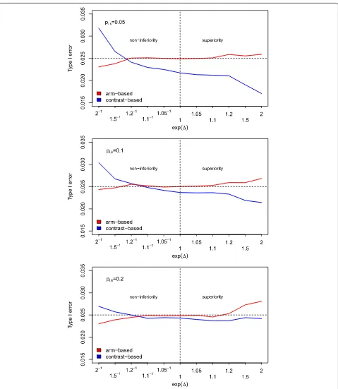
Type I error rate: The main interest was whether the approach maintains the type I error rate. In Fig. 1, the results of the first part of the simulation studies are shown.

Table 1Number of events and number of observations per trial for the illustrative data example (yikandNik,k=A,B,C,D, respectively) [6,26]

A B C D

ID yiA NiA yiB NiB yiC NiC yiD NiD

1 9 140 23 140 10 138

2 11 78 12 85 29 170

3 79 702 77 694

4 18 671 21 535

5 8 116 19 146

6 75 731 363 714

7 2 106 9 205

8 58 549 237 1561

9 1 33 9 48

10 3 100 31 98

11 1 31 26 95

12 6 39 17 77

13 95 1107 134 1031

14 15 187 35 504

15 78 584 73 675

16 69 1177 54 888

17 64 642 107 761

18 5 62 8 90

19 20 234 34

20 1 20 9 20

21 20 49 16 43

22 7 66 32 127

23 12 76 20 74

24 9 55 3 26

Fig. 1Simulated type I error rates. Simulated type I error rates for varying values of(based on 50,000 runs). The sample size per treatment arm and the success rate were kept fixed atNik=500 andpik=0.05, 0.1, 0.2, respectively (i=1,. . ., 16,k=P,S,E)

in some other situations the contrast-based approach is more conservative or liberal, respectively.

In the setting with 1,000 observations per treatment arm and study and values for very close to 0, both

these values are more common in practice. In all these sce-narios, the arm-based approach seems to perform slightly better than the contrast-based one, since it is less conser-vative but still maintains the type I error rate. Sometimes, the type I error rate was slightly above the nominal level. However, this exceedance can be regarded as negligible. In the last scenario, where extreme-values were used, one can see that the contrast-based approach inflates the type I error rate in a non-inferiority setting while it is very conservative in the superiority trials. In contrast, the arm-based approach maintains the type I error rate in (even extreme) non-inferiority scenarios but inflates the type I error rate in a superiority setting. Table 2summarizes these results.

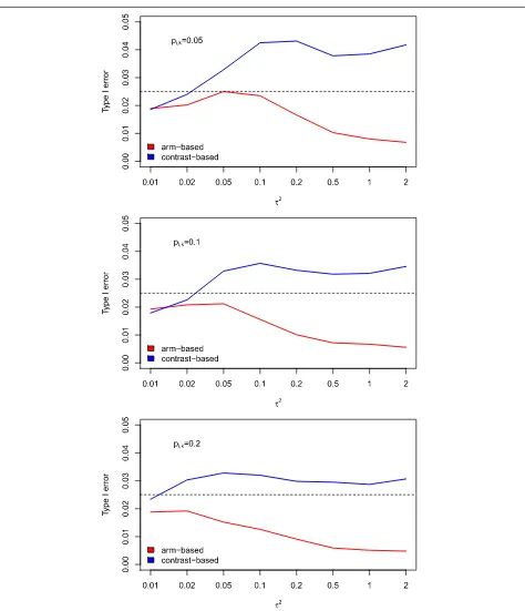
When introducing heterogeneity, we saw that the results for the two approaches (arm-based and contrast-based) were more different. The arm-based approach always maintains the type I error rate but becomes very con-servative in case of strong heterogeneity (see Fig. 2). The contrast-based approach, however, leads to slightly increased type I error rates for higher values of hetero-geneity. Lowering the sample size to 50 patients per study did not, in general, lead to inflated type I error rates when the arm-based approach was used. Only in case of strong heterogeneity the type I error was slightly inflated, or the test behaved slightly too conservative in the situa-tion of strong heterogeneity. In contrast, the effect-based approach led to an increased type I error rate in case of strong heterogeneity.

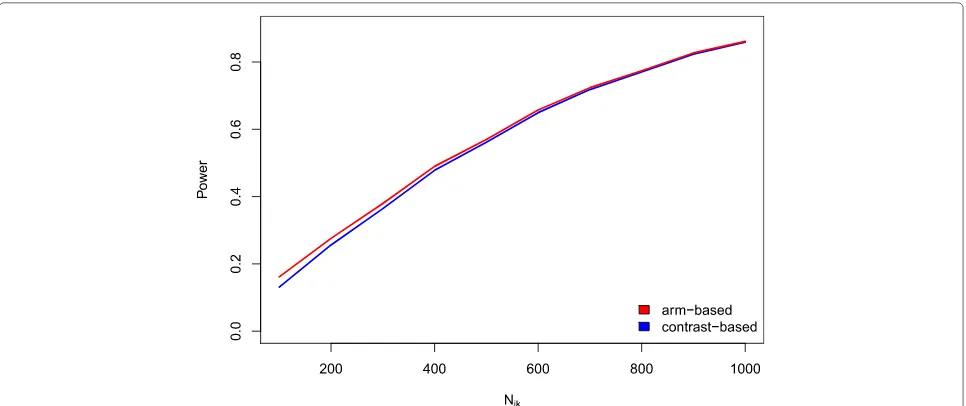
Power The investigations of the power showed that both approaches have a very similar performance. The arm-based approach resulted in slightly higher power com-pared to the contrast-based one (see Fig.3). The difference

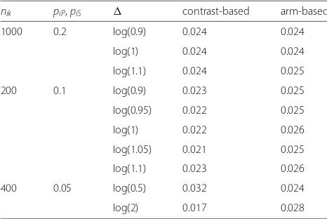
Table 2Simulated type I error rates of the testing approach in specific scenarios

nik piP,piS contrast-based arm-based

1000 0.2 log(0.9) 0.024 0.024

log(1) 0.024 0.024

log(1.1) 0.024 0.025

200 0.1 log(0.9) 0.023 0.025

log(0.95) 0.022 0.025

log(1) 0.022 0.026

log(1.05) 0.021 0.025

log(1.1) 0.023 0.026

400 0.05 log(0.5) 0.032 0.024

log(2) 0.017 0.028

nikdenotes the number of treatment arms,piPandpiSthe success rates in armP

andS, respectively, in triali(i=1,. . ., 16), andis the non-inferiority or superiority margin, respectively. We used 50,000 simulated data sets to estimate the type I error rate. The nominal level ofαwas 0.025

decreased with increasing sample size. This was to be expected since the type I error rates of the arm-based approach were also slightly increased compared to the contrast-based one. However, one has to keep in mind that the arm-based method did not maintain the significance level in some situations and thus has to be used with care.

Real data example

In Table 3, we provide the results for the data exam-ple. The estimated values forυ resulting from the arm-based and the contrast-arm-based approach are presented for each pair of hypotheses. We can see that the arm-based approach always leads to a higher value of υˆ than the contrast-based approach. If the cut-off for a test deci-sion of 0.975 is applied, the following test decideci-sions result. The first null hypothesisH0,1cannot be rejected for both

approaches. This means that the group counseling and the individual counseling are not significantly different. The second null hypothesis (H0,2) can be rejected according to

both approaches that means that the individual counseling is significantly more effective than self-help. The third null hypothesis (H0,3) can be rejected with the arm-based but

not when applying the contrast-based approach. Since we could see from our simulation study that the arm-based approach leads to type I error rates that are very close to the nominal level, the arm-based should be a proper choice. However, the safe (but maybe too conservative) option would be to apply the contrast-based approach and thus to maintain the null hypothesis in this case.

Discussion

Fig. 2Simulated type I error rates (heterogeneity). Simulated type I error rates for varying values ofτ2_{(based on 10,000 runs). The sample size per} treatment arm and the success rate were kept fixed atNik=500 andpik=0.05, 0.1, 0.2, respectively (i=1,. . ., 16,k=P,S,E), whilewas set to 0

on the type I error rate. However, even when the sample size was lowered to 50 patients per arm and trial, the type I error was still very close to the nominal level and only deviated slightly from it in case of strong heterogeneity. It

Fig. 3Power values. Power for the arm-based and contrast-based approach for a varying sample sizeNi,k(based on 10,000 runs). The success rate was kept fixed atpik=0.1 while the number of observations was varied (i=1,. . ., 16;k=P;S;E). An OR of 1.15 was used for power simulation while=0 was used

There are some limitations of our simulation study. Of course, there are by far more data situations as those considered. However, we covered a range of common situ-ations in medical research. There is also a lot of discussion about inconsistency in NMA models in the literature (see, for example, Dias et al. [29], or Krahn et al. [30]). In our simulation scenarios, it was assumed that there is no inconsistency present in the data which is a limitation of our study. Consistency is an assumption typically made in a standard NMA model but might be problematic in practice. In recent publications, this issue was addressed and solutions were proposed by applying more complex models [31–35]. However, in this work we focused on the standard NMA model. Note that when examining the type I error rate, the null hypothesis is assumed to hold true. Thus, the success rates in all treatment arms are exactly the same by design (or the same plus a pre-defined) and therefore there is no inconsistency per definition.

A test decision can also be based on the 95% credi-ble intervals around the point estimate of the log OR. If is not included, the null hypothesis can be rejected. We compared this approach to the methods suggested in this article. The type I error rate tended to be slightly

Table 3Resulting values forυˆfor the illustrative data example using the contrast-based and the arm-based approach

Contrast-based Arm-based

H0,1vs.H1,1: 0.685 0.759

H0,2vs.H1,2: >0.999 >0.999

H0,3vs.H1,3: 0.972 0.990

increased if the test decision was based on the credible interval compared to the approach based onυbut overall the results were very similar. Thus, it is not a considerable improvement compared to a test decision based on the credible intervals but rather a complement on the existing methodology.

Conclusions

In conclusion, we proposed and discussed an index that can be used to test for superiority or non-inferiority of a treatment arm compared to another one within a Bayesian NMA. The estimation is done during the NMA model estimation and does not result in any (noticeable) addi-tional computaaddi-tional cost. At the same time, the imple-mentation is very easy. Obviously, this approach can also be applied in a straightforward way in any other data sit-uation than binary data, as continuous data or a survival time, and is therefore a flexible tool.

done before applying the approach discussed here or, in general, any NMA approach. It is hardly possible to define an approach that is valid and optimal for any situation in practice and we emphasize the limitations of the approach described in this paper.

Abbreviations

NMA: Network meta-analysis; OR: Odds-ratio

Acknowledgements

We acknowledge financial support by Deutsche Forschungsgemeinschaft and Ruprecht-Karls-Universität Heidelberg within the funding programme Open Access Publishing. Furthermore, we would like to thank the editors and reviewers for their valuable proposals and comments that considerably improved our manuscript in different aspects.

Funding

Open Access Publishing was funded by Deutsche Forschungsgemeinschaft and Ruprecht-Karls-Universität Heidelberg within the funding programme Open Access Publishing.

Availability of data and materials

All data analyzed in our illustrative example are included in this published article.

Authors’ contributions

LU wrote the first draft of the manuscript, conducted the simulation study and applied the approach to the illustrative data example. KJ and MK contributed to the writing, and critically commented and revised the applied methods and the manuscript. All authors revised and approved the final version of the manuscript.

Ethics approval and consent to participate

Not applicable.

Consent for publication

Not applicable.

Competing interests

The authors declare that they have no competing interests.

Publisher’s Note

Springer Nature remains neutral with regard to jurisdictional claims in published maps and institutional affiliations.

Received: 13 July 2017 Accepted: 15 October 2018

References

1. Efthimiou O, Debray T, Valkenhoef G, Trelle S, Panayidou K, Moons KG, Reitsma JB, Shang A, Salanti G, GetReal Methods Review Group. Getreal in network meta-analysis: a review of the methodology. Res Synth Methods. 2016;7:236–63.

2. Dias S, Sutton AJ, Ades A, Welton NJ. Evidence synthesis for decision making 2: a generalized linear modeling framework for pairwise and network meta-analysis of randomized controlled trials. Med Dec Making. 2013;33:607–17.

3. Dias S, Welton NJ, Sutton AJ, Caldwell DM, Lu G, Ades AE. Evidence synthesis for decision making 4: inconsistency in networks of evidence based on randomized controlled trials. Med Dec Making. 2013;33:641–56. 4. Rücker G, Schwarzer G. Ranking treatments in frequentist network

meta-analysis works without resampling methods. BMC Med Res Methodol. 2015;15:58.

5. Higgins JPT, Whitehead A. Borrowing strength from external trials in a meta-analysis. Stat Med. 1996;15:2733–49.

6. Lu G, Ades A. Assessing evidence inconsistency in mixed treatment comparisons. J Am Stat Assoc. 2006;101:447–59.

7. Salanti G. Special issue on network meta-analysis. Res Synth Methods. 2012;2:69–190.

8. Bradburn MJ, Deeks JJ, Berlin JA, Russell Localio A. Much ado about nothing: a comparison of the performance of meta-analytical methods with rare events. Stat Med. 2007;26:53–77.

9. Lane PW. Meta-analysis of incidence of rare events. Stat Methods Med Res. 2013;22:117–32.

10. Sweeting MJ, Sutton AJ, Lambert PC. What to add to nothing? Use and avoidance of continuity corrections in meta-analysis of sparse data. Stat Med. 2004;23:1351–75.

11. Higgins J, Deeks J, Altman D. Chapter 16: Special topics in statistics. In: Higgins S, Green S, editors. Cochrane Handbook for Systematic Reviews of Interventions Version 5.1.0 (updated March 2011). The Cochrane Collaboration, 2011; 2011. Available fromhttp://handbook.cochrane.org/. Accessed 12 May 2016.

12. Kawasaki Y, Miyaoka E. A bayesian inference of p(π1> π2) for two proportions. J Biopharm Stat. 2012;22:425–37.

13. Kawasaki Y, Miyaoka E. A bayesian non-inferiority test for two independent binomial proportions. Pharm Stat. 2013;12:201–6.https:// doi.org/10.1002/pst.1571.

14. Nikolakopoulou A, Mavridis D, Egger M, Salanti G. Continuously updated network meta-analysis and statistical monitoring for timely

decision-making. Stat Methods Med Res. 2018;27:1312–30. 15. Datta GS, Sweeting TJ. Probability matching priors. Technical Report,

Research Report No. 252. 2005. Department of Statistical Science, University College London.

16. Rücker G, Schwarzer G, Krahn U, König J. Netmeta: Network

Meta-Analysis Using Frequentist Methods. 2015. R package version 0.8-0, http://CRAN.R-project.org/package=netmeta. Accessed 25 Aug 2016. 17. Friede T, Röver C, S W, Neuenschwander B. Meta-analysis of few small

studies in orphan diseases. Res Synth Meth. 2017;8:79–91. 18. Song F, Clark A, Bachmann MO, Maas J. Simulation evaluation of

statistical properties of methods for indirect and mixed treatment comparisons. BMC Med Res Methodol. 2012;12:138.

19. R Core Team. R: A Language and Environment for Statistical Computing. Vienna, Austria: R Foundation for Statistical Computing; 2012. R Foundation for Statistical Computing.http://www.R-project.org/. Accessed 25 Aug 2016.

20. Plummer M. Rjags: Bayesian Graphical Models Using MCMC. 2013. R package version 3-11,http://CRAN.R-project.org/package=rjags. Accessed 25 Aug 2016.

21. Revolution Analytics, Weston S. doSNOW: Foreach Parallel Adaptor for the Snow Package. 2014. R package version 1.0.12,http://CRAN.R-project. org/package=doSNOW.

22. Revolution Analytics. Foreach: Foreach Looping Construct for R. 2012. R package version 1.4.0,http://CRAN.R-project.org/package=foreach. Accessed 25 Aug 2016.

23. Plummer M, Best N, Cowles K, Vines K. Coda: convergence diagnosis and output analysis for mcmc. R News. 2006;6:7–11.

24. Revolution Analytics. Iterators: Iterator Construct for R. 2012. R package version 1.0.6,http://CRAN.R-project.org/package=iterators. Accessed 25 Aug 2016.

25. Dahl DB. Xtable: Export Tables to LaTeX or HTML. 2014. R package version 1.7-4,http://CRAN.R-project.org/package=xtable. Accessed 25 Aug 2016. 26. Hasselblad V. Meta-analysis of multitreatment studies. Med Dec Making.

1998;18:37–43.

27. Smoking Cessation Guideline Panel. Smoking Cessation, Clinical Practice Guideline No. 18 (AHCPR Publication No. 96-0692). Rockville: MD: Agency for Health Care Policy and Research, U.S. Department of Health and Human Services; 1996.

28. Gelman A. Comment: Fuzzy and bayesian p-values and u-values. Statist Sci. 2005;20:380–1.

29. Dias S, Welton NJ, Caldwell DM, Ades AE. Checking consistency in mixed treatment comparison meta-analysis. Stat Med. 2010;29:932–44.https:// doi.org/10.1002/sim.3767.

30. Krahn U, Binder H, König J. A graphical tool for locating inconsistency in network meta-analyses. BMC Med Res Methodol. 2013;13:35.

31. Jackson D, Barrett J, Rice S, White I, Higgins J. A design-by-treatment interaction model for network meta-analysis with random inconsistency effects. Stat Med. 2014;33:3639–54.

33. Jackson D, Law M, Barrett J, Turner R, Higgins J, Salanti G, White I. Extending dersimonian and laird’s methodology to perform network meta-analyses with random inconsistency effects. Stat Med. 2016;35: 819–39.

34. Jackson D, Veroniki A, Law M, Tricco A, Baker R. Paule-mandel estimators for network meta-analysis with random inconsistency effects. Res Synth Methods. 2017;8:416–34.