Analyzing Tensor Power Method Dynamics
in Overcomplete Regime
Animashree Anandkumar [email protected]
Department of Electrical Engineering and Computer Science University of California, Irvine
Engineering Hall, Room 4408 Irvine, CA 92697, USA
Rong Ge [email protected]
Department of Computer Science Duke University
308 Research Drive (LSRC Building), Room D226 Durham, NC 27708, USA
Majid Janzamin [email protected]
Department of Electrical Engineering and Computer Science University of California, Irvine
Engineering Hall, Room 4406 Irvine, CA 92697, USA
Editor:Tommi Jaakkola
Abstract
We present a novel analysis of the dynamics of tensor power iterations in the overcomplete regime where the tensor CP rank is larger than the input dimension. Finding the CP decomposition of an overcomplete tensor is NP-hard in general. We consider the case where the tensor components are randomly drawn, and show that the simple power iteration recovers the components with bounded error under mild initialization conditions. We apply our analysis to unsupervised learning of latent variable models, such as multi-view mixture models and spherical Gaussian mixtures. Given the third order moment tensor, we learn the parameters using tensor power iterations. We prove it can correctly learn the model parameters when the number of hidden componentsk is much larger than the data dimensiond, up tok =o(d1.5). We initialize the power iterations with data samples and
prove its success under mild conditions on the signal-to-noise ratio of the samples. Our analysis significantly expands the class of latent variable models where spectral methods are applicable. Our analysis also deals with noise in the input tensor leading to sample complexity result in the application to learning latent variable models.
Keywords: tensor decomposition, tensor power iteration, overcomplete representation, unsupervised learning, latent variable models
c
1. Introduction
CANDECOMP/PARAFAC (CP) decomposition of a symmetric tensor T ∈Rd×d×d is the process of decomposing it into a succinct sum of rank-one tensors, given by
T = X
j∈[k]
λjaj⊗aj⊗aj, λj ∈R, aj ∈Rd, (1)
where⊗denotes the outer product. The minimumkfor which the tensor can be decomposed in the above form is called the (symmetric) tensor rank. Tensor power iterationis a simple, popular and efficient method for recovering the tensor rank-one componentsaj’s. The tensor power iteration is given by
x← T(I, x, x)
kT(I, x, x)k, (2)
where
T(I, x, x) := X j,l∈[d]
xjxlT(:, j, l)∈Rd
is amultilinearcombination of tensorfibers, andk·kis the`2norm operator. See Section 1.3 for an overview of tensor notations and preliminaries.
The tensor power iteration is a generalization of matrix power iteration: for matrix
M ∈ Rd×d, the power iteration is given by x ← M x/kM xk. Dynamics and convergence properties of matrix power iterations are well understood (Horn and Johnson, 2012). On the other hand, a theoretical understanding of tensor power iterations is much more limited. Tensor power iteration can be viewed as a gradient descent step (with infinite step size), corresponding to the problem of finding the best rank-1 approximation of the input tensor
T (Anandkumar et al., 2014c). This optimization problem is non-convex. Unlike the matrix case, where the number of isolated stationary points of power iteration is at most the dimension (given by eigenvectors corresponding to unique eigenvalues), in the tensor case, the number of stationary points is, in fact, exponential in the input dimension (Cartwright and Sturmfels, 2013). This makes the analysis of tensor power iteration far more challenging. Despite the above challenges, many advances have been made in understanding the tensor power iterations in specific regimes. When the components aj’s are orthogonal to one another, it is known that there are no spurious local optima for tensor power itera-tions, and the only stable fixed points correspond to the trueaj’s (Zhang and Golub, 2001; Anandkumar et al., 2014c). Any tensor with linearly independent components aj’s can be orthogonalized, via an invertible transformation (whitening) and thus, its components can be recovered efficiently. A careful perturbation analysis in this setting was carried out in Anandkumar et al. (2014c).
Overcomplete tensors also arise in many machine learning applications such as moments of many latent variable models, e.g., multiview mixtures, independent component Analysis (ICA), and sparse coding models, where the number of hidden variables exceeds the input dimensions (Anandkumar et al., 2015). Overcomplete models often have impressive em-pirical performance (Coates et al., 2011), and can provide greater flexibility in modeling, and are more robust to noise (Lewicki and Sejnowski, 2000). By studying algorithms for overcomplete tensor decomposition, we expand the class of models that can be learnt effi-ciently using simple spectral methods such as tensor power iterations. Note there are other algorithms for decomposing overcomplete tensors (De Lathauwer et al., 2007; Goyal et al., 2013; Bhaskara et al., 2013), but they all require tensors of at least 4-th order and require large computational complexity. Ge and Ma (2015) works for 3rd order tensor but requires quasi-polynomial time. The main contribution of this paper is an analysis for the practical power method in the overcomplete regime.
1.1 Summary of Results
We analyze the dynamics of third order tensor power iterations in the overcomplete regime. We assume that the tensor componentsaj’s are randomly drawn from the unit sphere. Since general tensor decomposition is challenging in the overcomplete regime, we argue that this is a natural first step to consider for tractable recovery.
We characterize the basin of attraction for the local optima near the rank-one compo-nents aj’s. We show that under mild initialization condition, there is fast convergence to these local optima inO(log logd) iterations. This result is the core technical analysis of this paper stated in the following theorem.
Theorem 1 (Dynamics of tensor power iteration) Consider tensor Tˆ=T +E such that exact tensorT has rank-k decomposition in (1)with rank-one componentsaj ∈Rd, j∈
[k]being uniformly i.i.d. drawn from the unit d-dimensional sphere, and the ratio of max-imum and minmax-imum (in absolute value) weights λj’s being constant. In addition, suppose
the perturbation tensor E has bounded spectral norm as
kEk ≤
√
k
d , where < o
√
k d
!
. (3)
Let tensor rank k = o(d1.5), and the unit-norm initial vector x(1) satisfy the correlation bound
|hx(1), aji| ≥dβ √
k
d , (4)
w.r.t. some true component aj, j∈[k], for some β >(logd)−c for some universal constant
c >0. AfterN = Θ (log logd) iterations, the tensor power iteration in (2)outputs a vector having w.h.p. a constant correlation with the true component aj as |hx(N+1), aji| ≥ 1−γ,
for any fixed constantγ >0.
The above result is a significant improvement over the recent analysis by Anandkumar et al. (2015, 2014a,b) for overcomplete tensor decomposition. In these works, it is required for the initialization vectors to have a constant amount of correlation with the true aj’s. However, obtaining such strong initializations is usually not realistic in practice. On the other hand, the initialization condition in (4) is mild, and decaying even when the rankkis significantly larger than dimensiond; up tok=o(d1.5). In learning the mixture model, such initialization vectors can be obtained as samples from the mixture model, even when there is a large amount of noise. Given this improvement, we combine our analysis in Theorem 1, and the guarantees in Anandkumar et al. (2015, 2014a), proving that the model parameters can be recovered consistently.
A detailed proof outline for Theorem 1 is provided in Section 3.1. Under the random assumption, it is not hard to show that the first iteration of tensor power update makes progress. However, after the first iteration, the input vector and the tensor components are no longer independent of each other. Therefore, we cannot directly repeat the same argument for the second step.
How do we analyze the second step even though the vector and tensor components are correlated? The main intuition is to characterize the dependency between the vector and the tensor components, and show that there is still enough randomness left for us to repeat the argument. This idea was inspired by the analysis of Approximate Message Passing (AMP) algorithms (Bayati and Montanari, 2010). However, our analysis here is very different in several key aspects: 1) In approximate message passing, typically the analysis works in the
large system limit, where the number of iterations is fixed and the dimension goes to infinity. Here we can handle a superconstant number of iterationsO(log logd), even for finite d; 2) Usually kis assumed to be a constant factor times din the AMP-like analysis, while here we allow them to be polynomially related.
1.2 Related Work
Tensor decomposition for learning latent variable models: In the introduction, some related works are mentioned which study the theoretical and practical aspects of spectral techniques for learning latent variable models. Among them, Anandkumar et al. (2014c) provide the analysis of tensor power iteration for learning several latent variable models in the undercomplete regime. Anandkumar et al. (2014a) provide the analysis in the overcomplete regime and Anandkumar et al. (2014b) provide tensor concentration bounds and apply the analysis in (Anandkumar et al., 2014a) to learning LVMs proposing tight sample complexity guarantees.
Distance-based methods impose separation condition on the mean vectors showing that under enough separation the parameters can be estimated. Among such approaches, we can mention Dasgupta (1999); Vempala and Wang (2002); Arora and Kannan (2005). As discussed in the summary of results, these results work even if k > d1.5 as long as the separation condition between means is satisfied, but our work can tolerate higher level of noise in the regime of k = o(d1.5) with polynomial computational complexity. The guarantees in (Vempala and Wang, 2002) also work in the high noise regime but need higher computational complexity as polynomial inkO(k) and d.
In the spectral approaches, the observed moments are constructed and the spectral de-composition of the observed moments are performed to recover the parameters (Kalai et al., 2010; Anandkumar et al., 2012, 2014b). Kalai et al. (2010) analyze the problem of learning mixture of two general Gaussians and provide algorithm with high order polynomial sample and computational complexity. Note that in general, the complexity of such methods grows exponentially with the number of components without further assumptions (Moitra and Valiant, 2010). Hsu and Kakade (2013) provide a spectral algorithm under non-degeneracy conditions on the mean vectors and propose guarantees with polynomial sample complexity depending on the condition number of the moment matrices. Anandkumar et al. (2014b) perform tensor power iteration on the third order moment tensor to recover the mean vectors in the overcomplete regime as long as k=o(d1.5), but need very good initialization vector having constant correlation with the true mean vector. Here, we improve the correlation level required for convergence.
1.3 Notation and Tensor Preliminaries
Let [k] := {1,2, . . . , k}, and kvk denote the `2 norm of vector v. We use ˜O and ˜Ω to hide polylog factors in asymptotic notationsO and Ω, respectively.
Tensor preliminaries: A real p-th order tensor T ∈ NpRd is a member of the outer
product of Euclidean spaces Rd. The different dimensions of the tensor are referred to as
modes. For instance, for a matrix, the first mode refers to columns and the second mode refers to rows. In addition, fibers are higher order analogues of matrix rows and columns. A fiber is obtained by fixing all but one of the indices of the tensor (and is arranged as a column vector). For example, for a third order tensorT ∈Rd×d×d, the mode-1 fiber is given by T(:, j, l). Similarly,slices are obtained by fixing all but two of the indices of the tensor. For example, for the third order tensorT, the slices along 3rd mode are given by T(:,:, l).
We view a tensorT ∈Rd×d×d as a multilinear form. In particular, for vectors u, v, w∈
Rd, we have1
T(I, v, w) := X j,l∈[d]
vjwlT(:, j, l) ∈Rd, (5)
which is a multilinear combination of the tensor mode-1 fibers. SimilarlyT(u, v, w)∈Ris a
multilinear combination of the tensor entries, andT(I, I, w)∈Rd×dis a linear combination of the tensor slices.
A 3rd order tensor T ∈Rd×d×d is said to be rank-1 if it can be written in the form
T =λ·a⊗b⊗c⇔T(i, j, l) =λ·a(i)·b(j)·c(l), (6)
h
z1 z2 · · · zp
Figure 1: Multiview mixture model.
where notation ⊗ represents the outer productand a, b, c ∈Rd are unit vectors. A tensor
T ∈Rd×d×d is said to have a CPrank at mostk if it can be written as the sum ofkrank-1 tensors as
T = X
i∈[k]
λiai⊗bi⊗ci, λi∈R, ai, bi, ci∈Rd. (7)
For third order tensor T ∈Rd×d×d, the spectral (operator) norm is defined as
kTk:= sup
kuk=kvk=kwk=1
|T(u, v, w)|.
In the rest of the paper, Section 2 describes how to apply our tensor results to learning multiview mixture models. Section 3 illustrates the proof ideas, with more details in the Appendix. Finally we conclude in Section 4.
2. Learning Multiview Mixture Model through Tensor Methods
We proposed our main technical result in Section 1.1 providing convergence guarantees for the tensor power iterations given mild initialization conditions in the overcomplete regime; see Theorem 1. Along this result we provide the application to learning multiview mixtures model in Theorem 2. In this section, we briefly introduce the tensor decomposition frame-work as the learning algorithm and then state the learning guarantees with more details and remarks.
2.1 Multiview Mixture Model
Consider an exchangeable multiview mixture model withkcomponents andp≥3 views; see Figure 1. Suppose that hidden variable h is a discrete categorical random variable taking one of the kstates. It is convenient to represent it by basis vectors such that
h=ej ∈Rk if and only if it takes thej-th state.
Note that ej ∈ Rk denotes the j-the basis vector in the k-dimensional space. The prior
probability for each hidden state is Pr[h=ej] =λj, j∈[k]. For simplicity, in this paper we assume all the λi’s are the same. However, similar argument works even when the ratio of maximum and minimum prior probabilitiesλmax/λmin is bounded by some constant.
The variables (views) zl ∈ Rd are related to the hidden state through factor matrix A∈Rd×k such that
Algorithm 1 Learning multiview mixture model via tensor power iterations Require: 1) Third order moment tensorT ∈Rd×d×din (8), 2)nsamples ofz
1in multiview mixture model asz(τ)1 , τ ∈[n], and 3) number of iterationsN.
1: forτ = 1 tondo
2: Initialize unit vectorsx(1)τ ←z1(τ)/ z
(τ) 1
.
3: for t= 1 toN do
4: Tensor power updates (see (5) for the definition of the multilinear form):
x(t+1)τ =
TI, x(t)τ , x(t)τ
T
I, x(t)τ , x(t)τ
, (9)
5: end for
6: end for
7: return the output of Procedure 2 with input n
x(Nτ +1):τ ∈[n] o
as estimatesxj.
where zero-mean noise vectors ηl∈Rdare independent of each other and the hidden state h. Given this, the variables (views) zl ∈Rd are conditionally independent given the latent
variableh, and the conditional means areE[zl|h=ej] =aj, whereaj ∈Rddenotes thej-th
column of factor matrix A = [a1· · ·ak] ∈ Rd×k. In addition, the above properties imply
that the order of observations zl do not matter and the model is exchangeable. The goal of the learning problem is to recover the parameters of the model (factor matrix) A given observations.
For this model, the third order2 observed moment has the form (Anandkumar et al., 2014c)
E[z1⊗z2⊗z3] = X
j∈[k]
λjaj⊗aj ⊗aj. (8)
Hence, given third order observed moment, the unsupervised learning problem (recovering factor matrixA) reduces to computing a tensor decomposition as in (8).
2.2 Tensor Decomposition Algorithm
The algorithm for unsupervised learning of multiview mixture model is based on tensor decomposition techniques provided in Algorithm 1. The main step in (9) performs tensor power iteration;3 see (5) for the multilinear form definition. After running the algorithm for all different initialization vectors, the clustering process from Anandkumar et al. (2015) ensures that the best converged vectors are returned as the estimation of true components
aj.
Procedure 2 Clustering process (Anandkumar et al., 2015) Require: TensorT ∈Rd×d×d, set S:=nx(N+1)
τ :τ ∈[n] o
, parameterν.
1: whileS is not empty do
2: Choose x∈S which maximizes|T(x, x, x)|.
3: DoN more iterations of (9) starting from x.
4: Output the result of iterations denoted by ˆx.
5: Remove all the x∈S with |hx,xˆi|> ν/2.
6: end while
2.3 Learning Guarantees
We assume a Gaussian prior on the mean vectors, i.e., the vectorsaj ∼ N(0, Id/d), j∈[k] are i.i.d. drawn from a standard multivariate Gaussian distribution with unit expected square norm. Note that in the high dimension (growingd), this assumption is the same as uniformly drawing from unit sphere since the norm of vector concentrates in the high dimen-sion and there is no need for normalization. Even though we impose a prior distribution, we do not use a MAP estimator, since the corresponding optimization is NP-hard. Instead, we learn the model parameters through decomposition of the third order moments through tensor power iterations. The assumption of a Gaussian prior is standard in machine learning applications. We impose it here for tractable analysis of power iteration dynamics. Such Gaussian assumptions have been used before for analysis of other iterative methods such as approximate message passing algorithms, and there are evidences that similar results hold for more general distributions; see (Bayati and Montanari, 2010) and references there.
As explained in the previous sections, we use tensor power method to learn the compo-nentsaj’s, and the method is initialized with observed sampleszi. Intuitively, this initializa-tion is useful sincezi =Ah+ηi is a perturbed version of desired parameteraj (whenh=ej). Thus, we present the result in terms of the signal-to-noise (SNR) ratio which is the expected norm of signal aj (which is one here) divided by the expected norm of noise ηi, i.e., the SNR in thei-th samplezi =aj+ηi (assumedh=ej) is defined as SNR :=E[kajk]/E[kηik]. This specifies how much noise the initialization vector zi can tolerate in order to ensure the convergence of tensor power iteration to a desired local optimum. We now propose the conditions required for recovery guarantees, and state a brief explanation of them.
Conditions for Theorems 2 and 3:
• Rank condition: k≤o(d1.5).
• The columns ofA are uniformly i.i.d. drawn from unitd-dimensional sphere.
• The noise vectorsηl, l∈[3], are independent of matrixAand each other. In addition, the signal-to-noise ratio (SNR) is w.h.p. bounded as
SNR≥Ω p
max{k, d}
d1−β !
,
The rank condition bounds the level of overcompleteness for which the recovery guar-antees are satisfied. The random assumption on the columns ofA are crucial for analyzing the dynamics of tensor power iteration. We use it to argue there exists enough random-ness left in the components after conditioning on the previous iterations; see Section 3.1 for the details. The bound on the SNR is required to make sure the given sample used for initialization is close enough to the corresponding mean vector. This ensures that the initial vector is inside the basin-of-attraction of the corresponding component, and hence, the convergence to the mean vector can be guaranteed. Under these assumptions we have the following theorem.
Theorem 2 (Learning multiview mixture model: closeness to single columuns)
Consider a multiview mixture model (or a spherical Gaussian mixture) in the above settings with k components in d dimensions. If the above conditions hold, then the tensor power iteration converges to a vector close to one of the true mean vectors aj’s (having constant
correlation).
In particular, for mildly overcomplete models, where k=αd for some constantα >1, the signal-to-noise ratio (SNR) is as low as Ω(d−1/2+), for any >0. Thus, we can learn mixture models with a high level of noise. In general, we establish how the required noise level scales with the number of hidden componentsk, as long as k=o(d1.5).
The above theorem states convergence to desired local optima which are close to true componentsaj’s. In Theorem 3, we show that we can sharpen the above result, by jointly iterating over the recovered vectors, and consistently recover the components aj’s. This result also uses the analysis from Anandkumar et al. (2015).
Theorem 3 (Learning multiview mixture model: recovering the factor matrix)
Assume the above conditions hold. The initialization of power iteration is performed by samples of z1 in multiview mixture model. Suppose the tensor power iterations are at least
initialized once for eachaj, j∈[k]such thatz1 =aj+η1.4 Then by using the exact 3rd order
moment tensor in (8) as input, the tensor decomposition algorithm outputs an estimate Aˆ
(up to permutation of its columns) satisfying w.h.p. (over the randomness of the components
aj’s)
ˆ
A−A
F ≤,
where the number of iterations of the algorithm is N = Θ log 1
+ log logd
.
See Section 3 for the proof.
The above theorems assume the exact third order tensor is given to the algorithm. We provide the results given empirical tensor in Section 2.3.1.
Learning spherical Gaussian mixtures: Consider a mixture of k different Gaussian vec-tors with spherical covariance. Let aj ∈ Rd, j ∈ [k] denote the mean vectors and the
covariance matrices areσ2I. Assuming the parameter σ is known, the modified third order observed moment
M3 :=E[z⊗z⊗z]−σ2
X
i∈[d]
(E[z]⊗ei⊗ei+ei⊗E[z]⊗ei+ei⊗ei⊗E[z])
has the tensor decomposition form (Hsu and Kakade, 2012)
M3= X
j∈[k]
λjaj⊗aj⊗aj,
where λj is the probability of drawing j-th Gaussian mixture. The above guarantees can be applied to learning mean vectorsaj in this model with the additional property that the noise is spherical Gaussian.
Learning multiview mixture model with distinct factor matrices: Consider the multiview mixture model with different factor matrices where the first three views are related to the hidden state as
z1=Ah+η1, z2=Bh+η2, z3 =Ch+η3.
Then, the guarantees in the above theorem can be extended to recovering the columns of all three factor matricesA,B, andC with appropriate modifications in the power iteration algorithm as follows. First the update formula (9) is changed as
x(t+1)1,τ =
TI, x(t)2,τ, x(t)3,τ
T
I, x(t)2,τ, x(t)3,τ
, x(t+1)2,τ =
Tx(t)1,τ, I, x(t)3,τ
T
x(t)1,τ, I, x(t)3,τ
, x(t+1)3,τ =
Tx(t)1,τ, x(t)2,τ, I
T
x(t)1,τ, x(t)2,τ, I
,
which is the alternating asymmetric version of symmetric power iteration in (9). Here, we alternate among different modes of the tensor. In addition, the initialization for each mode of the tensor is appropriately performed with the samples corresponding to that mode. Note that the analysis still works in the asymmetric version since there exists even more independence relationships through the iterations of the power update because of introducing new random matrices B and C.
2.3.1 Sample Complexity Analysis
In the previous section, we assumed the exact third order tensor in (8) is given to the tensor decomposition Algorithm 1. We now estimate the tensor given nsamples z1(i), z2(i), z3(i), i∈ [n], as
ˆ
T = 1
n
X
i∈[n]
z1(i)⊗z(i)2 ⊗z3(i). (10)
For the multiview mixture model introduced in Section 2.1, let the noise vector ηl be spherical, and ζ2 denote the variance of each entry of noise vector. We now provide the following recovery guarantees.
Additional conditions for Theorem 4:
• Let E1 := [η1(1), η (2) 1 , . . . , η
(n)
1 ] ∈ Rd×n, where η (i)
1 ∈ Rd is the i-th sample of noise vector η1. These noise matrices satisfy the following RIP property which is adapted from Candes and Tao (2006). MatrixE1∈Rd×n satisfies a weak RIP condition such
that for any subset ofOlogd2d
• The number of samples nsatisfies lower bound such that
ζ
√
d
n +
r
λmax
d n
!
+ζ2 d n+
r
λmax
d1.5
n
!
+ζ3 d
1.5
n +
r
d n
! ≤min
(
√
k
d ,O˜(λmin)
)
, (11)
where < o√k/d.
Theorem 4 (Learning multiview mixture model) Consider the empirical tensor in
(10) as the input to tensor decomposition Algorithm 1. Suppose the above additional condi-tions are also satisfied. Then, the same guarantees as in Theorem 2 hold. In addition, the same guarantees as in Theorem 3 also hold with the recovery bound (up to permutation of columns ofAˆ) changed as
ˆ
A−A
F
≤O˜
√
k· kEk
λmin !
,
where E denotes the perturbation tensor originated from empirical estimation in (10), and its spectral norm kEk is bounded by the LHS of (11).
See Section 3 for the proof.
3. Proof Outline
Our main technical result is the analysis of third order tensor power iteration provided in Theorem 1 which also allows to tolerate some amount of noise in the input tensor. We analyze the noiseless and noisy settings in different ways. We basically first prove the result for the noiseless setting where the input tensor has an exact rank-k decomposition in (1). When the noise is also considered, we show that the contribution of noise in the analysis is dominated by the main signal, and thus, the same result still holds. For the rest of this section we focus on the noiseless setting, while we discuss the proof ideas for the noisy case in Section 3.2.
We first discuss the proof of Theorem 3 which involves two phases. In the first phase, we show that under certain small amount of correlation (see (13)) between the initial vector and the true component, the power iteration in (2) converges to some vector which has constant correlation with the true component. This result is the core technical analysis of this paper which is provided in Lemma 5. In the second phase, we incorporate the result of Anandkumar et al. (2015, 2014a) which guarantees the convergence of power iteration (followed by a coordinate descent iteration) given initial vectors having constant correlation with the true components. This is stated in Lemma 6.
To simplify the notation, we consider the tensor5
T = X
j∈[k]
aj⊗aj ⊗aj, aj ∼ N(0, 1
dId). (12)
Notice that this is exactly proportional to the 3rd order moment tensor of the multiview mixture model in (8).
The following lemma is restatement of Theorem 1 in the noiseless setting.
Lemma 5 (Dynamics of tensor power iteration, phase 1) Consider the rank-k ten-sorT of the form in (12). Let tensor rankk=o(d1.5), and the unit-norm initial vector x(1)
satisfies the correlation bound
|hx(1), aji| ≥dβ √
k
d , (13)
w.r.t. some true component aj, j∈[k], for some β >(logd)−c for some universal constant
c >0. AfterN = Θ (log logd) iterations, the tensor power iteration in (2)outputs a vector having w.h.p. a constant correlation with the true component aj as
|hx(N+1), aji| ≥1−γ,
for any fixed constantγ >0.
The proof outline of above lemma is provided in Section 3.1. Next, we provide the following lemma from Anandkumar et al. (2015) which provides the dynamics of tensor power iteration when the initialization satisfies the constant correlation bound stated below.
Lemma 6 (Dynamics of tensor power iteration, phase 2) Consider the rank-k ten-sorT of the form in (12) with rank conditionk≤o(d1.5). Let the initial vectorsx(1)
j satisfy
the constant correlation bound
|hx(1)j , aji| ≥1−γj,
w.r.t. true components aj, j ∈[k], for some constants γj >0. Let the output of the tensor
power updates6 in (2)applied to all these different initialization vectors afterN = Θ log1
iterations be stacked as columns of matrix Aˆ. Then, we have w.h.p.7
Aˆ−A
F ≤,
where the recovery error is up to permutation of columns of Aˆ.
See Anandkumar et al. (2015) for the proof of above lemma. Given the above two lemmas, the learning result in Theorem 3 is directly proved.
Proof of Theorem 3 The result is proved by combining Lemma 5 and Lemma 6. Note that the initialization condition in (4) is w.h.p. satisfied given the SNR bound assumed.
Proof of Theorem 4 In Theorem 3, we provided the result given exact tensor by combin-ing Lemmas 5 and 6. The only difference here is we are given an empirical estimate of the tensor and we need to incorporate the effect of noise in the empirical input. We now use
6. This result also needs an additional step of coordinate descent iterations since the true components are not the fixed points of power iteration; see Anandkumar et al. (2015, 2014a) for the details.
Theorem 1 that characterizes the effect of noise in first step (adapting Lemma 5 to noisy setting), and Anandkumar et al. (2015) that provide the result of Lemma 6 in noisy setting. In addition, the tensor concentration bound for multiview mixture model is analyzed in Theorem 1 of Anandkumar et al. (2014b) (Lemma 56 in Anandkumar et al. (2015)) that shows the error between empirical and exact tensors is bounded as
kTˆ−Tk ≤ζ
√
d
n +
r
λmax
d n
!
+ζ2 d n+
r
λmax
d1.5
n
!
+ζ3 d
1.5
n +
r
d n
!
.
The sample complexity requirement in (11) is then derived by imposing the error require-ments in our noisy analysis of tensor power dynamics in Theorem 1 (see Equation (3)) and the noisy analysis of Lemma 6 (see Theorem 1 of Anandkumar et al. (2015) where the perturbation tensor E needs to be bounded as kEk ≤ O˜(λmin)). The final recovery error on
Aˆ−A
F is also from Theorem 1 of Anandkumar et al. (2015).
3.1 Proof Outline of Lemma 5 (Noiseless Case of Theorem 1)
First step: We first intuitively show the first step of the algorithm makes progress. Suppose the tensor isT =P
j∈[k]aj⊗aj⊗aj, and the initial vectorxhas correlation|hx, a1i| ≥dβ
√
k d with the first component. The result of the first iteration is the normalized version of the following vector:
˜
x= X
j∈[k]
haj, xi2aj.
Intuitively, this vector should have roughlyha1,x˜i=d2β kd2 correlation witha1 (as the other terms are random they don’t contribute much). On the other hand, the norm of this vector is roughly O(√k/d): this is because haj, xi2 for j 6= 1 is roughly8 1/d, and the sum of k random vectors with length 1/dwill have length roughlyO(√k/d). These arguments can be made precise showing the normalized version ˜x/kx˜khas correlationd2β
√
k
d witha1 ensuring progress in the first step.
Going forward: As we explained, the basic idea behind proving Lemma 5 is to character-ize the conditional distribution of random Gaussian tensor componentsaj’s given previous iterations. In particular, we show that the residual independent randomness left in these conditional distributions is large enough and we can exploit it to obtain tighter concentra-tion bounds throughout the analysis of the iteraconcentra-tions. The Gaussian assumpconcentra-tion on the components, and small enough number of iterations are crucial in this argument.
Notations: For two vectors u, v ∈ Rk, the Hadamard product denoted by ∗ is defined
as the entry-wise multiplication of vectors, i.e., (u∗v)j := ujvj for j ∈ [k]. For a matrix
A, let P⊥A denote the projection operator to the subspace orthogonal to column span of
A. For a subspace R, let R⊥ denote the space orthogonal to it. Therefore, for a subspace
R, the projection operator on the subspace orthogonal toRis equivalently denoted byPR⊥
orP⊥R. For a random matrix D, letD|{u=Dv} denote the conditional distribution ofD
given linear constraintsu=Dv. We also use equality notation(d)= to denote the equivalence in distribution.
Lemma 5 involves analyzing the dynamics of power iteration in (2) for 3rd order rank-k
tensors. For the rank-ktensor in (12), the power iterative formx← kTT(I,x,x)(I,x,x)k can be written as
x(t+1)= A A
>x(t)∗2
A A
>x(t)∗2
, (14)
where the multilinear form in (5) is used. Here, A= [a1· · ·ak]∈Rd×k denotes the factor
matrix, and for vector y ∈ Rk, y∗2 := y ∗y ∈
Rk represents the element-wise square of
entries ofy.
We consider the case whereai ∼ N(0,1dI) are i.i.d. drawn and we analyze the evolution of the dynamics of the power update. As explained earlier, for a given initialization x(1), the update in the first step can be analyzed easily since Ais independent ofx(1). However, in subsequent steps, the updatesx(t) are dependent on A, and it is no longer clear how to provide a tight bound on the evolution ofx(t). In this work, we provide a careful analysis by controlling the amount of “correlation build-up” by exploiting the structure of Gaussian matrices under linear constraints. This enables us to provide better guarantees for matrix
A with Gaussian entries compared to general matricesA.
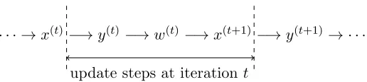
Intermediate update steps and variables:Before we proceed, we need to break down power update in (2) and introduce some intermediate update steps and variables as follows. Recall that x(1) ∈ Rd denotes the initialization vector. Without loss of generality, let us analyze the convergence of power update to first component of rank-k tensor T denoted by a1. Hence, let the first entry ofx(1) denoted byx(1)1 be the maximum entry (in absolute value) of x(1), i.e., x(1)1 =kx(1)k∞. LetB := [a2 a3 · · · ak]∈Rd×(k−1), and thereforeA= [a1|B]. We break the power update formula in (2) into a few steps by introducing intermediate variables y(t)∈Rk and ˜x(t+1) ∈
Rd as
y(t):=A>x(t), x˜(t+1):=A(y(t))∗2.
Note that ˜x(t+1) is the unnormalized version of x(t+1) := ˜x(t+1)/kx˜(t+1)k, i.e., ˜x(t+1) :=
T(I, x(t), x(t)). Thus, we need to jointly analyze the dynamics of all variables x(t),y(t) and (y(t))∗2. Define
X[t]:=hx(1)|. . .|x(t)i, Y[t]:=hy(1)|. . .|y(t)i.
Matrix B is randomly drawn with i.i.d. Gaussian entries Bij ∼ N(0,1d). As the iterations proceed, we consider the following conditional distributions
B(t,1) :=B|{X[t], Y[t]}, B(t,2):=B|{X[t+1], Y[t]}. (15) Thus,B(t,1)is the conditional distribution ofB at the middle oftth iteration (before update
step ˜x(t+1)=A(y(t))∗2) and B(t,2) is the conditional distribution at the end oftth iteration
3.1.1 Conditional Distributions
In order to characterize the conditional distribution ofB under evolution ofx(t) andy(t)in (15), we exploit the following basic fact (see (Bayati and Montanari, 2010) for proof).
Lemma 7 (Conditional distribution of Normal matrices under linear condition)
Consider random matrix D with i.i.d. Gaussian entries Dij ∼ N(0, σ2). Conditioned on
u=Dv with known vectorsu and v, the matrixD is distributed as
D|{u=Dv}(d)= 1 kvk2uv
>+ ˜DP⊥
v,
where random matrix D˜ is an independent copy of D with i.i.d. Gaussian entries D˜ij ∼ N(0, σ2), and P⊥v is the projection operator on to the subspace orthogonal to v.
We refer to ˜DP⊥v as the residual random matrix since it represents the remaining
randomness left after conditioning. It is a random matrix whose rows are independent random vectors that are orthogonal to v, and the variance in each direction orthogonal to
v is equal to σ2.
The above Lemma can be exploited to characterize the conditional distribution of B
introduced in (15). However, a naive direct application using the constraint Y[t]=A>X[t]
is not transparent for analysis. The reason is the evolution of x(t) and y(t) are themselves governed by the conditional distribution ofB given previous iterations. Therefore, we need the following recursive version of Lemma 7 which can be immediately argued by induction.
Corollary 8 (Iterative conditioning) Consider random matrix D with i.i.d. Gaussian entries Dij ∼ N(0, σ2), and let F
(d)
=P⊥CDP⊥R be the random Gaussian matrix whose columns are orthogonal to spaceC and rows are orthogonal to spaceR. Conditioned on the linear constraint u=Dv, where9 u∈C⊥, the matrix F is distributed as
F|{u=Dv}(d)= 1
k(P⊥Rv)k2u(P⊥Rv)
>+P⊥
CDP⊥˜ {R,v},
where random matrix D˜ is an independent copy of D with i.i.d. Gaussian entries D˜ij ∼ N(0, σ2).
Thus, the residual random matrix P⊥CDP⊥˜ {R,v} is a random Gaussian matrix whose columns are orthogonal toC and rows are orthogonal to span{R, v}. The variance in any remaining dimension is equal toσ2.
3.1.2 Form of Iterative Updates
Now we exploit the conditional distribution arguments proposed in the previous section to characterize the conditional distribution ofB given the update variablesxand y up to the current iteration; recall (15) whereB(t,1) is the conditional distribution ofB at the middle oftth iteration andB(t,2) at the end oftth iteration. Before that, we need to introduce some
more intermediate variables.
Intermediate variables: We separate the first entry ofy and (y)∗2 from the rest, i.e., we have
y1(t)=a>1x(t), y(t)−1 =B>x(t)∼(B(t−1,2))>x(t),
where y(t)−1 ∈Rk−1 denotesy(t) ∈
Rk with the first entry removed. The update formula for
˜
x(t+1) can be also decomposed as ˜
x(t+1)= (y1(t))2a1+Bw(t)∼(y(t)1 )2a1+B(t,1)w(t), where
w(t):= (y(t)−1)∗2 ∈Rk−1,
is the new intermediate variable in the power iterations. Let Bres.(t,1) and Bres.(t,2) denote the
residualrandom matrices corresponding to B(t,1) and B(t,2) respectively, and
u(t+1) :=Bres.(t,1)w(t), v(t):= (B(tres.−1,2))>x(t),
where u(t) ∈ Rd and v(t) ∈
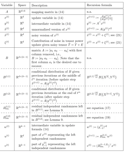
Rk−1 are respectively the part of x(t) and y(t)−1 representing the residual randomness after conditioning on the previous iterations. We also summarize all variables and notations in Table 1 in the Appendix which can be used as a reference throughout the paper.
Finally we make the following observations.
Lemma 9 (Form of iterative updates) The conditional distribution of B at the middle of tth iteration denoted byB(t,1) satisfies
B(t,1) (d)= X i∈[t−1]
u(i+1)(P⊥
W[i−1]w (i))>
kP⊥
W[i−1]w
(i)k2 + X
i∈[t]
P⊥
X[i−1]x
(i)(v(i))>
kP⊥
X[i−1]x
(i)k2 +B (t,1)
res. , (16)
Bres.(t,1)(d)=P⊥
X[t]
˜
BP⊥
W[t−1], (17)
where random matrix B˜ is an independent copy of B with i.i.d. Gaussian entries B˜ij ∼ N(0,d1). Similarly, the conditional distribution of B at the end of tth iteration denoted by B(t,2) satisfies
B(t,2) (d)=X i∈[t]
u(i+1)(P⊥
W[i−1]w (i))>
kP⊥
W[i−1]w
(i)k2 +
P⊥
X[i−1]x
(i)(v(i))>
kP⊥
X[i−1]x (i)k2
!
+Bres.(t,2), (18)
B(t,2)res. (d)=P⊥
X[t]B
0P⊥
W[t], (19)
where random matrix B0 is an independent copy of B with i.i.d. Gaussian entries Bij0 ∼ N(0,d1).
· · · →x(t) −→y(t)−→w(t) −→x(t+1) −→y(t+1)→ · · · update steps at iteration t
Figure 2: Flow of the power update algorithm stating intermediate steps. Iteration t for which the inductive step should be argued is also indicated.
3.1.3 Analysis of Iterative Updates
Lemma 9 characterizes the conditional distribution of B given the update variables x and
y up to the current iteration; see (15) for the definition of conditional forms of B denoted by B(t,1) and B(t,2). Intuitively, when the number of iterations t d, then the resid-ual independent randomness left in B(t,1) and B(t,2) (respectively denoted by Bres.(t,1) and
Bres.(t,2)) characterized in Lemma 9 is large enough and we can exploit it to obtain tighter concentration bounds throughout the analysis of the iterations.
Note that the goal is to show that under t d, the iterations x(t) converge to the true component with constant error, i.e., |hx(t), a1i| ≥ 1−γ for some constant γ > 0. If this already holds before iteration t we are done, and if it does not hold, next iteration is analyzed to finally achieve the goal. This analysis is done via induction argument. During the iterations, we maintain several invariants to analyze the dynamics of power update. The goal is to ensure progress in each iteration as in (20).
Induction hypothesis: The following are assumed at the beginning of the iteration tas induction hypothesis; see Figure 2 for the scope of inductive step.
1. Length of Projection on x:
δt≤ kP⊥ X[t−1]x
(t)k ≤1,
whereδtis of order 1/polylogd, and the value ofδt only depends ont and logd.
2. Length of Projection on w:
δ0t−1
√
k
d ≤ kP⊥W[t−2]w
(t−1)k ≤∆0
t−1 √
k d ,
kP⊥
W[t−2]w (t−1)k
∞≤∆0t−1 1
d,
3. Progress:10
|ha1, x(t)i| ∈[δ∗t,∆
∗
t]dβ2 t−1
√
k
d , (20)
|ha1, P⊥ X[t−1]x
(t)i| ≤∆∗
tdβ2 t−1
√
k d .
4. Norm of u,v:
δt−1 2
r
k d ≤ kv
(t−1)k ≤2 r
k d, δt0−1
2 √
k d ≤ ku
(t)k ≤2∆0
t−1 √
k d .
The analysis for basis of induction and inductive step are provided in Appendix B.
3.2 Effect of Noise in Theorem 1
Given rank-krandom tensorT in (12), and a starting pointx(1), our analysis in the noiseless setting shows that the tensor power iteration in (2) outputs a vector which will be close to
aj ifx(1) has a large enough correlation with aj.
Now suppose we are given noisy tensor ˆT =T +E where E has some small norm. In this case where the noise is also present, we get a sequence ˆx(t)=x(t)+ξ(t) wherex(t) is the component not incorporating any noise (as in previous section11), whileξ(t) represents the contribution of noise tensorE in the power iteration; see (21) below. We prove thatξ(t) is a very small noise that does not change our calculations stated in the following lemma.
Lemma 10 (Bounding norm of error) Suppose the spectral norm of the error tensorE
is bounded as
kEk ≤
√
k/d, where < o( √
k/d).
Then the noise vector ξ(t) at iteration tsatisfies the `2 norm bound kξ(t)k ≤O˜(dβ2t−1).
Note that when tis the first number such that dβ2t−1 ≥d/√k, we have kξ(t)k=o(1). Notice that since whendβ2t−1 ≥d/√k, the main induction is already over and we know
x(t) is constant close to the true component, and thus, the noise is always small.
Proof idea: We now provide an overview of ideas for proving the above lemma; see Appendix D for the complete proof which is based on an induction argument. We first
10. Note that although the bounds ony(−t)1 are argued at iteration t, the bound on the first entry of y (t)
denoted byy(1t)=ha1, x(t)iis assumed here in the induction hypothesis at the end of iterationt−1.
11. Note that there is a subtle difference between notationx(t) in the noiseless and noisy settings. In the noiseless setting, this vector is normalized, while in the noisy setting the whole vector ˆx(t)=x(t)+ξ(t)
write the following recursion expanding the contribution of main signal and noise terms in the tensor power iteration as
x(t+1)+ξ(t+1) = Norm
ˆ
T(x(t)+ξ(t), x(t)+ξ(t), I)
= NormT(x(t), x(t), I) + 2T(x(t), ξ(t), I) +T(ξ(t), ξ(t), I) +E(ˆx(t),xˆ(t), I),
(21)
where for vectorv, we have Norm(v) :=v/kvk, i.e., it normalizes the vector. The first term is the desired main signal and should have the largest norm, and the rest of the terms are the noise terms. The third term is of orderkξ(t)k2, and hence, it should be fine whenever we choosekEkto be small enough. The last term isO(kEk) and is the same for all iterations so that is also fine. The problematic term is the second term, whose norm if we bound naively is 2kξ(t)k. However the normalization factor also contributes a factor of roughly d/√k, and thus, this term grows exponentially; it is still fine if we just do a constant number of iterations, but the exponent will depend on the number of iterations.
In order to solve this problem, and make sure that the amount of noise we can tolerate is independent of the number of iterations, we need a better way to bound the noise termξ(t). The main problem here is we bound the norm ofkT(x(t), ξ(t), I)kbykTkkξ(t)k ≤O(ξ(t)), by doing this we ignored the fact thatx(t) is uncorrelated with the components inT. In order to get a tighter bound, we introduce another normk·k∗; see Definition 21 for the exact form.
Intuitively, the norm k · k∗ captures the fact that x does not have a high correlation with
the components (except for the first component thatxwill converge to), and gives a better bound. In particular we have kT(x(t), ξ(t), I)k ≈
√
k
d kξ(t)k2. Therefore, the normalization factor is compensated by the additional term
√
k d .
4. Conclusion
In this paper, we provide a novel analysis for the dynamics of third order tensor power iteration showing convergence guarantees to vectors having constant correlation with the tensor component. This enables us to prove unsupervised learning of latent variable models in the challenging overcomplete regime where the hidden dimensionality is larger than the observed dimension. The main technical observation is that under random Gaussian tensor components and small number of iterations, the residual randomness in the components (which are involved in the iterative steps) are sufficiently large. This enables us to show progress in the next iteration of the update step. As future work, it is very interesting to generalize this analysis to higher order tensor power iteration, and more generally to other kinds of iterative updates.
Acknowledgments
Variable Space Description Recursion formula
A Rd×k mapping matrix in (14) n.a.
x(t) Rd update variable in (14) x(t+1) := kA(yA(y((tt))))∗∗22k y(t) Rk intermediate variable in (14) y(t):=A>x(t)
˜
x(t) Rd unnormalized version ofx(t) x˜(t+1) :=A(y(t))∗2 ˆ
x(t) Rd noisy version of x(t) xˆ(t) =x(t)+ξ(t); see (21)
ξ(t) Rd Contribution of noise in tensor power
update given noisy tensor ˆT =T +E xˆ
(t) =x(t)+ξ(t); see (21)
B Rd×(k−1)
matrixA:= [a1 a2 · · · ak] with first column removed, i.e.,
B := [a2 a3 · · · ak]. Note that the first columna1 is the desired one to recover.
n.a.
B(t,1) Rd×(k−1)
conditional distribution of B given previous iterations at the middle of
tth iteration (before update step
˜
x(t+1)=A(y(t))∗2)
B(t,1) (d)=B|{X[t], Y[t]}
B(t,2) Rd×(k−1)
conditional distribution of B given previous iterations at the end of tth
iteration (after update step ˜
x(t+1)=A(y(t))∗2)
B(t,2) (d)=B|{X[t+1], Y[t]}
Bres.(t,1) Rd×(k−1) residual independent randomness left
inB(t,1); see Lemma 9. see equation (17)
Bres.(t,2) Rd×(k−1) residual independent randomness left
inB(t,2); see Lemma 9. see equation (19)
w(t)
Rk−1 intermediate variable in update
formula (14) w
(t):= (y(t)
−1)∗2
u(t) Rd part ofx
(t) representing the left
independent randomness u
(t+1) :=B(t,1) res. w(t)
v(t) Rk−1 part ofy
(t)
−1 representing the left
independent randomness v
(t):= (B(t−1,2) res. )>x(t)
Appendix A. Proof of Lemma 9
Proof of Lemma 9 Recall that we have updates of the form
˜
x(t+1)=A(y(t))∗2, w(t):= (y−(t)1)∗2, y(t)=A>x(t).
Let
X[t]\1 :=hx(2)|. . .|x(t)i,
and let the rows ofY[t] are partitioned as the first and the rest of rows as
Y[t]=
Y1[t]>
Y
[t]
−1
>>
.
We now make the following simple observations
B(t,1) (d)=B|{Y[t]=A>X[t],X˜[t]\1 =A(Y[t−1])∗2} (d)
=B|{Y−[t]1 =B>X[t],X˜[t]\1 =a1(Y1[t−1])∗2+BW[t−1]} (d)
=B|{v(1)=B>x(1), . . . , v(t)= (Bres.(t−1,2))>x(t), u(2) =B(1,1)res. w(1), . . . , u(t)=B(tres.−1,1)w(t−1)},
where the second equivalence comes from the fact that B is matrix A with first column removed. Now applying Corollary 8, we have the result. The distribution of B(t,2) follow similarly.
Appendix B. Analysis of Induction Argument
In this section, we analyze the basis of induction and inductive step for the induction argument proposed in Section 3.1.3 for the proof of Lemma 5.
B.1 Basis of Induction
We first show that the hypothesis holds for initialization vectorx(1)as the basis of induction.
Claim 1 (Basis of induction) The induction hypothesis is true for t= 1.
B.2 Inductive Step
Assuming the induction hypothesis holds for all the values till the end of iteration t−1 (stated in Section 3.1.3), we analyze the t-th iteration of the algorithm, and prove that induction hypothesis also holds for the values at the end of iterationt. See Figure 2 where the scope of iteration tand the flow of the algorithm is shown. In the rest of this section, we pursue the flow of the algorithm at iterationt starting from computing y(t) and ending up with computing x(t+1) to prove the desired induction hypothesis at iteration t.
B.2.1 Hypothesis 4
We start by showing that the induction Hypothesis 4 holds at iterationtusing the induction Hypotheses 1 and 2 in the previous iteration.
Claim 2 We have
δt 2
r
k d ≤ kv
(t)k ≤2 r
k d, δ0t
2 √
k d ≤ ku
(t+1)k ≤2∆0
t √
k d .
Proof Recall that v(t):= (Bres.(t−1,2))>x(t), and by applying the form ofB(tres.−1,2) in (19), we have
v(t) (d)=P⊥
W[t−1]B
0>P⊥
X[t−1]x
(t). (22)
Since random matrixB0 ∈Rd×(k−1)is an independent copy ofB with i.i.d. Gaussian entries
Bij0 ∼ N(0,1d), we know v(t) is a random Gaussian vector in the subspace orthogonal to
W[t−1]. On the other hand, for any vector z∈Rd, we have
E
h
kB0>zk2i=z>E
h
B0B0>iz= k−1
d kzk
2, where EB0B0> = k−d1I is exploited. Let z = P⊥
X[t−1]x
(t). Then, by applying the above equality to the expansion ofv(t) in (22), we have
E
h
kv(t)k2i= k−t
k−1 ·
k−1
d · kP⊥X[t−1]x
(t)k2 = k−t
d · kP⊥X[t−1]x (t)k2 ∈
δt2k d
1− t
k ,k d ,
where dim(W[t−1]) =t−1 is also used in the first step, and the last step is concluded from Hypothesis 1. Finally, by concentration property of random Gaussian vectors, when td
we have with high probability
kv(t)k ∈ "
δt 2
r
k d,2
r
k d
#
.
Similarly, for u(t+1) :=B(t,1)
res. w(t), and by applying the form of Bres.(t,1) in (17), we have
u(t+1) (d)=P⊥
X[t]
˜
BP⊥
W[t−1]w
Since random matrix ˜B ∈Rd×(k−1) is an independent copy ofB with i.i.d. Gaussian entries ˜
Bij ∼ N(0,1d), we know u(t+1) is a random Gaussian vector in the subspace orthogonal to
X[t]. On the other hand, for any vector z∈Rk−1, we have
E
h
kBz˜ k2i=z> E
h ˜
B>B˜iz=kzk2,
where E
h ˜
B>B˜i = I is exploited. Let z = P⊥
W[t−1]w
(t). Then, by applying the above equality to the expansion ofu(t+1) in (23), we have
E
h
ku(t+1)k2i= d−t
d · kP⊥W[t−1]w (t)k2∈
(δt0)2 k
d2
1− t
d
,(∆0t)2 k
d2
,
where dim(X[t]) = t is also used in the first step, and the last step is concluded from Hypothesis 2. Finally, by concentration property of random Gaussian vectors, when td
we have with high probability
ku(t+1)k ∈ "
δt0
2 √
k d ,2∆
0 t √ k d # .
B.2.2 Hypothesis 2
Computing y(t): In the first step of iteration t, the algorithm computes y(t). By induction Hypothesis 3, we know|y1(t)|= ˜Θ(dβ2t−1√k/d). The other coordinates ofy(t) :=A>x(t) are
y−(t)1 =B>x(t)which conditioning on the previous iterations are equivalent (in distribution) to
y(t)−1(d)=B(t−1,2) > x(t) = X
i∈[t−1]
u(i+1)(P⊥
W[i−1]w (i))>
kP⊥
W[i−1]w
(i)k2 +
P⊥
X[i−1]x
(i)(v(i))>
kP⊥
X[i−1]x (i)k2
!
+Bres.(t−1,2)
>
x(t)
= X
i∈[t−1] ˜ Θ d2 k P⊥
W[i−1]w
(i)hu(i+1), x(t)i+ ˜Θ(1)v(i)hP⊥ X[i−1]x
(i), x(t)i
+v(t), (24)
where form of B(t−1,2) in (18) is used in the second equality. The bounds on the norms come from Hypotheses 1 and 2. The last term is by definitionv(t) := (Bres.(t−1,2))>x(t). Note that differences in polylog factors in the (upper and lower) bounds in Hypotheses 1 and 2 are represented by notation ˜Θ(·).
We will establish subsequently that if k > d, the terms involving v(i)’s in the above expansion dominate, and the terms involving P⊥
W[i−1]w
Computing w(t): In the next step of the algorithm at iteration t, w(t) is computed for which we now argue if the induction hypothesis holds up to iteration t, both lower and upper bounds at iterationtaskP⊥
W[t−1]w
(t)k ∈[δ0
t,∆0t]
√
k
d (see induction Hypothesis 2) also hold.
Lower bound: For the lower bound, intuitively thefreshrandom vectorv(t)should bring enough randomness into w(t). We formulate that in the following lemma.
Lemma 11 SupposeRandR0are two subspaces inRkwith dimension at mostt≤ 16(logkk)2. Let p ∈ Rk be an arbitrary vector, z ∈
Rk be a uniformly random Gaussian vector in the
space orthogonal to R, and finallyw= (p+z)∗(p+z). Then with high probability, we have
kP⊥R0wk ≥
E[kzk2]
40√k .
Recall thatw(t):=y−(t)1∗y−(t)1, andy−(t)1 is expanded in (24) as sum of an arbitrary vector and a random Gaussian vector. Applying above lemma with R = R0 = span(W[t−1]), we have with high probability
kP⊥
W[t−1]w
(t)k ≥ E[kv(t)k2] 40√k ≥
δt2
160 √
k/d,
where Hypothesis 4 gives lower bound kv(t)k ≥δt/2 p
k/d(used in the second inequality). By choosingδt0 =δ2t/160 the lower bound in Hypothesis 2 is proved.
Upper bound: In order to prove the upper bounds in Hypothesis 2, we follow the sequence of arguments below:
Claim 3: ky−(t)1k∞
(·)2
==⇒ kw(t)k∞======Lemma 12⇒ kP⊥
W[t−1]w (t)k
∞⇒ kP⊥
W[t−1]w (t)k
First we prove a bound on the infinity norm of y−(t)1: Claim 3 (Upper bound on ky−(t)1k∞) We have
ky−(t)1k∞≤ t δt
logd
√
d + (t−1)
∆0t−1
δ0t−1
2 1 √
k = ˜O
1 √
d
.
Proof We exploit the induction hypothesis to bound the`∞ norm of all the terms in the expansion of y(t)−1 in (24).
For the terms involving v(i), since they are random Gaussian vectors with expected square norm at most k/d, by Lemma 19 we know kv(i)k∞≤ log√d
d with high probability. In addition, forv(i),i < t, the coefficient is bounded as
hP⊥
X[i−1]x
(i), x(t)i kP⊥
X[i−1]x
(i)k2 ≤
1 kP⊥
X[i−1]x (i)k ≤
1
δi
where the last step uses Hypothesis 1. Therefore, the total contribution from terms involving
v(i) inky−(t)1k∞ is bounded by δt
t log√d
d. For the terms involvingP⊥
W[i−1]w
(i), i∈[t−1], we have from Hypothesis 2 that the `∞ norm is bounded as kP⊥
W[i−1]w (i)k
∞ ≤ ∆0i1d. In addition, the corresponding coefficient is
bounded by
hu(i+1), x(t)i kP⊥
W[i−1]w (i)k2 ≤
ku(i+1)k · kx(t)k kP⊥
W[i−1]w (i)k2 ≤
2∆0i
δi02 d
√
k. (26)
Again bounds in Hypotheses 2 and 4 are exploited in the last inequality. Hence, the total contribution from terms involving P⊥
W[i−1]w
(i), i ∈ [t−1] in ky(t)
−1k∞ is bounded by (t−
1) ∆0
t−1
δ0t−1
2 1
√
k.
Combining the above bounds finishes the proof.
Since w(t):=y(t)−1∗y−(t)1, the above claim immediately implies that kw(t)k∞≤O˜
1
d
. (27)
Now we have the `∞ norm on w, however we need to bound the`∞ norm of the projected vectorP⊥
W[t−1]w
(t). Intuitively this is clear as the vectors in the spaceW[t−1] all have small
`∞ as guaranteed by induction hypothesis. We formalize this intuition using the following lemma.
Lemma 12 Suppose R is a subspace in Rk of dimension t0, such that there is a basis
{r1, . . . , rt0} withkrik∞≤ √∆
k and krik= 1. Let p∈R
k be an arbitrary vector, then
kP⊥Rpk∞≤ kpk∞+kpk∆
√
t0
√
k.
Let R= span(W[t−1]). Then the vectorsP⊥
W[i−1]w
(i)/kP⊥ W[i−1]w
(i)k,i∈[t−1] form a basis for subspace R, and we know from Hypothesis 2 that the `∞ norm of each of these basis vectors is bounded by √∆
k for ∆ := ∆0
t−1
δ0
t−1 which is of order polylogd. Applying above
lemma, we have
kP⊥
W[t−1]w (t)k
∞≤ kw(t)k∞(1 + ∆
√
t−1)≤ ∆
0
t
d ,
where the last inequality uses bound (27), and appropriate choosing for ∆0twhich is of order polylogdand only depends ontand logd. This concludes the upper bound on the`∞norm in Hypothesis 2. The upper bound on the `2 norm is also immediately argued using this
`∞ norm bound where an additional√kfactor shows up.
B.2.3 Hypothesis 1
Computing x(t+1):
˜
x(t+1) (d)=B(t,1)w(t)+ (y1(t))2a1
= X
i∈[t−1]
u(i+1)(P⊥
W[i−1]w (i))>
kP⊥
W[i−1]w
(i)k2 w
(t)+X i∈[t]
P⊥
X[i−1]x
(i)(v(i))>
kP⊥
X[i−1]x
(i)k2 w (t)
+B(t,1)res. w(t)+ (y1(t))2a1
= X
i∈[t−1] ˜ Θ
d2 k
u(i+1)hP⊥
W[i−1]w
(i), w(t)i+X i∈[t]
˜ Θ(1)P⊥
X[i−1]x
(i)hv(i), w(t)i
+u(t+1)+ (y1(t))2a1, (28)
where form ofB(t,1) in (16) is used in the second equality. The bounds on the norms come from Hypotheses 1 and 2. The last term is the definition of u(t+1):=Bres.(t,1)w(t). Note that differences in polylog factors in the (upper and lower) bounds in Hypotheses 1 and 2 are represented by notation ˜Θ(·).
The goal is to prove Hypothesis 1 holds at t-th iteration (which is to show the desired lower and upper bounds onkP⊥
X[t]x
(t+1)k) assuming induction hypothesis holds for earlier iterations. Given the normalizationx(t+1) := ˜x(t+1)/kx˜(t+1)kin each iteration, we have
kP⊥
X[t]x
(t+1)k= 1
kx˜(t+1)kkP⊥X[t]x˜
(t+1)k. (29)
Therefore, we first bound the norm of ˜x(t+1) which turns out to be kx˜(t+1)k= ˜Θ
√
k d
as argued in the following.
Lower bound: The lower bound onkx˜(t+1)k simply follows from the term u(t+1), which is an independent random Gaussian.
Claim 4 If t≤ d
10, then we have whp
kx˜(t+1)k ≥ δ
0
t 4
√
k d .
Proof We have
kx˜(t+1)k ≥ kPspan(X[t],U[t],a 1)⊥x˜
(t+1)k=kP
span(X[t],U[t],a 1)⊥u
(t+1)k.
Note that the equality is concluded from expansion of ˜x(t+1) in (28) where all the com-ponents of ˜x(t+1) in the subspace span(X[t], U[t], a1)⊥ is represented byu(t+1). The vector
Pspan(X[t],U[t],a 1)⊥u
(t+1)is the projection of a random Gaussian vectoru(t+1) in to a subspace of dimentiond−o(d). Hence it is still a random Gaussian vector with expected square norm
larger than δ0t
2
2 k
d2. By Lemma 18, with high probability the desired bound holds.
Claim 5 We have either
hx(t+1), a1i ≥1−γ,
for some constant γ >0 or
kx˜(t+1)k ≤O˜
√
k d
!
.
Proof Let ˜x(t+1)in (28) be written as ˜x(t+1) =z+ (y1(t))2a1 where vectorz∈Rdrepresents
all the other terms in the expansion. The analysis is done under two cases 1) (y1(t))2≥ γ2kzk and 2) (y1(t))2 < γ2kzkfor some constantγ >0. Note that the left hand side is the norm of (y1(t))2a1 sinceka1k= 1, and in addition (y(t)1 )2 =hx(t), a1i2.
Case 1
(y(t)1 )2≥ γ2kzk: For thex(t+1) := ˜x(t+1)/kx˜(t+1)k, we have hx(t+1), a1i=
1
kz+ (y1(t))2a 1k
hz+ (y1(t))2a1, a1i
≥ 1
kzk+ (y1(t))2 h
(y1(t))2− kzki
≥ 1− γ 2
1 +γ2 ≥1−γ,
where triangle and Cauchy-Schwartz inequality are used in the first bound, and the second inequality is concluded from assumption (y1(t))2≥ γ2kzk.
Case 2
(y(t)1 )2 < 2γkzk: We exploit the induction hypothesis to bound the norm of all the terms in the expansion of ˜x(t+1) in (28).
For the terms involvingu(i+1), i∈[t], we haveku(i+1)k ≤2∆0i
√
k
d from Hypothesis 4 and the argument forku(t+1)k. In addition, foru(i+1),i∈[t−1], the coefficient is bounded as
hP⊥
W[i−1]w
(i), w(t)i kP⊥
W[i−1]w
(i)k2 ≤
kw(t)k kP⊥
W[i−1]w (i)k ≤
∆0t
δi0 , (30)
where Cauchy-Schwartz inequality is used in the first bound, and the bound in Hypothesis 2 and (27) are exploited in the last inequality. Therefore, the total contribution from terms
involvingu(i+1) inkx˜(t+1)k is bounded by 2(t−1)∆0t2 δ0
t
√
k d . For the terms involving P⊥
X[i−1]x
(i), i ∈ [t], we have kP⊥ X[i−1]x
(i)k ≤ 1, but the coef-ficient hv(i), w(t)i needs further analysis to be bounded which is done in Lemma 13 say-ing |hv(i), w(t)i| ≤ O˜
√ k d
. This implies that the total contribution from terms involving
P⊥
X[i−1]x
(i) in kx˜(t+1)kis bounded by ˜O
√
k d
.
Combining the above bounds and considering the assumption that the norm of (y1(t))2a1 in the expansion of ˜x(t+1) is dominated by the norm of other terms argued above, the proof is complete concluding that kx˜(t+1)k ≤O˜
√
k d
Lemma 13 Under the induction hypothesis (up to update stepx˜(t+1):=A(y(t))∗2 at itera-tion t), we have fori∈[t],
|hv(i), w(t)i| ≤O t3 (∆ 0
t−1)4 (δ0t−1)4δ2
t (logd)
√
k d
! = ˜O
√
k d
!
.
Using (29) and the fact that kx˜(t+1)k= ˜Θ
√
k d
, we have
kP⊥
X[t]x
(t+1)k ≥Θ˜
d
√
k
kPspan(X[t],U[t],a 1)⊥u
(t+1)k ≥ δt0 4,
where the boundkPspan(X[t],U[t],a 1)⊥u
(t+1)k ≥ δt0 4
√
k
d is also used. This finishes the proof that Hypothesis 1 holds.
B.2.4 Hypothesis 3
Finally we prove Hypothesis 3 at iteration t given earlier induction hypothesis. The first part of the hypothesis is proved in the following claim.
Claim 6 We have
|ha1, x(t+1)i| ∈[δ∗t+1,∆
∗
t+1]dβ2 t
√
k d .
Proof We first show the correlation bound on the unnormalized version as ha1,x˜(t+1)i. Looking at the expansion of ˜x(t+1) in (28), the correlation ha
1,x˜(t+1)i involves three types of terms emerging from (y1(t))2a1, u(i+1) and P⊥
X(i−1)x
(i). In the following, we argue the correlation from each of these terms where we observe that the correlation is dominated by the term (y(t)1 )2a1, and the rest of terms contribute much smaller amount.
For the term (y1(t))2a1, we have
ha1,(y(t)1 )2a1i= (y1(t))2 ∈[(δ
∗
t)2,(∆
∗
t)2]dβ2 t k
d2,
where the last part exploits induction Hypothesis 3 in the previous iteration.
For the terms involvingu(i+1), these vectors are random Gaussian vectors in a subspace (with dimension Ω(d)), and therefore, we have with high probability
ha1, u(i+1)i ≤E[ku(i+1)k]·O
logd
√
d
≤O˜
√
k d√d
! ≤O˜
k d2
,
where the correlation bound between two independent random Gaussian vectors in Ω(d )-dimension is used in the first inequality,12Hypothesis 4 is exploited in the second inequality, and finally last inequality is from assumptionk > d. In addition, the coefficient associated
12. For two independent random Gaussian vectorsp, q∈Rd, we have with high probabilityhp, qi ≤E[kpk]· E[kqk]·O
log√d
d