Cross-Domain Visual Representations via Unsupervised Graph Alignment

The Thirty-Third AAAI Conference on Artificial Intelligence (AAAI-19)

Cross-Domain Visual Representations via Unsupervised Graph Alignment

Baoyao Yang, Pong C. Yuen

Department of Computer Science, Hong Kong Baptist University, Hong Kong [email protected], [email protected]

Abstract

In unsupervised domain adaptation, distributions of visual representations are mismatched across domains, which leads to the performance drop of a source model in the tar-get domain. Therefore, distribution alignment methods have been proposed to explore cross-domain visual representa-tions. However, most alignment methods have not consid-ered the difference in distribution structures across domains, and the adaptation would subject to the insufficient aligned cross-domain representations. To avoid the misclassifica-tion/misidentification due to the difference in distribution structures, this paper proposes a novel unsupervised graph alignment method that aligns both data representations and distribution structures across the source and target domains. An adversarial network is developed for unsupervised graph alignment, which maps both source and target data to a fea-ture space where data are distributed with unified strucfea-ture criteria. Experimental results show that the graph-aligned vi-sual representations achieve good performance on both cross-dataset recognition and cross-modal re-identification.

1

Introduction

In machine learning and pattern recognition, the generaliza-tion ability of a model decreases in the test dataset with the deviation of distributions between the training and test datasets. To overcome the problem of dataset bias when la-bels are unavailable in the test dataset, unsupervised domain adaptation (UDA) (Gopalan, Li, and Chellappa 2011) has been proposed. Recent researches (e.g., (Sun, Feng, and Saenko 2016; Tzeng et al. 2017)) have shown that align-ing data distributions across the trainalign-ing dataset (source do-main) and the test dataset (target dodo-main) is a promising approach to obtain cross-domain representations for unsu-pervised domain adaptation. After distribution alignment, the cross-domain representations have similar distributions in the source and target domains, and therefore the target-domain generalization error is reduced.

To achieve the cross-domain representations, many un-supervised domain adaptation methods (Long et al. 2014b; 2015; Sun, Feng, and Saenko 2016; Sun and Saenko 2016) proposed to align the statistical measures (e.g., mean, vari-ances) across the source and target domains. These meth-ods perform well when source and target data are distributed

Copyright c2019, Association for the Advancement of Artificial Intelligence (www.aaai.org). All rights reserved.

Graph Alignment Source Domain Target Domain Training Target images Source images + Labels Source features Target features Spac e Alig

nmen t Source Domain Target Domain Domain_-invaria nt Features Domain-invariant Space Source Domain Target Domain Graph Alignment Domain-invariant Space Source CNN Target CNN Edge Alignment Node Alignment

Domain Discriminator Domain labels

Testing Target images Classifier Class label Target features Target CNN

Classifier Class label

Consistency loss Discrepancy

loss

Edges in target space Edges btw target features Edges btw source features

Similarity-based Edge Calculator Source Domain Target Domain Unsupervised Graph Alignment

Aligned Feature Space

Ɛ = Ɩ

Ɛ = Ɩ

Ɛ = Ɩ 2

2

1 Ɛ = Ɩ 1

Ɛ = Ɩ 1 Ɛ = Ɩ 1

Network for Unsupervised Graph Alignment

Training Target Images Source Images + Labels Source features Target features Source CNN Target CNN Edge Alignment Node Alignment Domain

Discriminator Domain loss

Testing Target images Classifier Class label Target features Target CNN

Classifier Classification loss

Consistency loss Discrepancy loss

Edges in target space Edges btw target features Edges btw source features

Target CNN Classifier Source CNN Domain Discriminator Trained Network Source Domain Target Domain

Network for Unsupervised Graph Alignment

Training Target Images Source Images + Labels Source Features Target Features Source CNN Target CNN Edge Alignment Node Alignment Domain

Discriminator Domain loss

Testing

Classifier

Class label

Target CNN

Classifier Classification loss

Consistency loss Discrepancy loss

Edges in target space Edges btw target features Edges btw source features

Target CNN Classifier Source CNN Domain Discriminator Trained Network

Target Images Source Images

Source CNN Matching score Matching Source Features Target Features

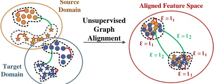
Figure 1: Basic idea of unsupervised graph alignment: Data are distributed with different structures in the source and target domains. Complete graphs are built in the source and target domains (edges are partially drawn) for align-ment. In the aligned feature space, nodes of source and tar-get data are closely located. The distribution structures are aligned across domains by constraining the values of source and target edges using the same criteria.

with structures (Tenenbaum, De Silva, and Langford 2000; Long et al. 2014a; Hou et al. 2016) that can be nicely re-produced by the mean and covariance. But this assumption is difficult to guarantee in real-world applications. When the assumption is invalid, data distributions in the source and target domains are failed to be aligned by merely shift-ing the means and/or covariances of the source and tar-get data. Other methods learned the cross-domain repre-sentations by subspace alignment (Fernando et al. 2013; Sun and Saenko 2015). Represented using the similar bases, source and target representations in the subspaces are re-garded as aligned. However, the source and target data in each subspace may be variously distributed with different distribution structures, resulting in a mismatch between dis-tributions of source and target data in the subspaces.

In this paper, we argue that data are distributed with different distribution structures (Tenenbaum, De Silva, and Langford 2000) in the source and target domains. That is, source/target data may be tightly or discretely located in the representation space without any prior geographic as-sumptions. Thus, the distribution alignment is insufficient in the existing methods that ignored the difference in distribu-tion structures. Instead, this paper proposes an unsupervised graph alignment method to explore cross-domain represen-tations, where source and target data have both similar rep-resentations and similar distribution structures. As shown in Figure 1, source data are linked to build a complete graph to represent the structural information of data distribution in the source domain. Similarly, a complete graph is built among target data. The values of edges in the source and tar-get graphs are the geometric distance (Wang and Mahadevan 2013) between each pairs of nodes (data representations) in each graph, and therefore, structural information of source and target distributions is recorded in the edges of source and target graphs, respectively. The distribution alignment across domains can then be modeled as the alignment between the source and target graphs. Domain-indiscrimination loss is adopted for node alignment. To achieve the edge alignment without target labels, unified criteria are designed for source and target edges in the feature space. The unified criteria constrain that values of source and target edges should be minimized or approach to a fixed distance. We also propose a consistency constraint to preserve the target structural in-formation among target features, so that arbitrary mapping of target data can be avoided with the guidance of the target structural information.

The contributions of this paper are listed as follows.

1. We propose an unsupervised graph alignment method to address the problem of structure difference in distribu-tion for unsupervised domain adaptadistribu-tion. The proposed method aligns representations of source and target data, while matching the distribution structures in the source and target domains.

2. We design unified criteria for edges in both source and target domains. Constrained by the unified edge criteria, edges that represent the structures of source and target distributions are aligned without target labels.

3. We develop an adversarial network to learn the graph-aligned representations with similar distribution struc-tures in the source and target domains. The graph-aligned representations not only are invariant to domains, but also preserve structural information in each domain.

2

Related Work

The problem of comparing distributions was addressed in (Gretton et al. 2007), and a statistic of Maximum Mean Discrepancy (MMD) was proposed to measure the proba-bility of two samples from different distributions. As unsu-pervised domain adaptation that aims to align distributions across the source and target domains has become popular in recent years, the technique of MMD has been applied in many unsupervised domain adaptation methods to ex-plore source and target features with similar distributions.

For example, source and target data are mapped to a domain-invariant feature space with the criterion of MMD in (Gong, Grauman, and Sha 2013; Long et al. 2014b); TSC (Long et al. 2013) and DsGsDL (Yang, Ma, and Yuen 2018) adopted MMD in dictionary learning models to obtain the aligned sparse representations; and (Long et al. 2015) formulated the criterion of MMD as a loss function in deep-learning models. However, (Sun, Feng, and Saenko 2016) found that merely matching the statistical measure of mean was not enough for distribution alignment, because the source and target data could also diverge in the covariance. Therefore, they proposed to align the second-order of statistics for un-supervised domain adaptation. Incorporating the convolu-tional network, (Sun and Saenko 2016) then extended this idea to a deep-learning version.

On the other hand, (Gopalan, Li, and Chellappa 2011) proposed a concept of domain shift that modeled the distri-bution alignment across the source and target domains as the shift of subspaces in the manifolds. The subspaces were also formulated as the bases in dictionary learning models in (Ni, Qiu, and Chellappa 2013), which aligned the source and tar-get domains by interpolating subspaces between the source and target domains. (Fernando et al. 2013) then summarized these methods as subspace alignment and represented the subspaces using eigenvectors extracted from PCA.

Besides, domain-indistinguishable features were pre-sented in (Ganin et al. 2016) to align distributions for un-supervised domain adaptation. (Ganin et al. 2016) believed that the source and target distributions were aligned in the domain-indistinguishable features. With the popularity of generative adversarial networks, adversarial adaptation net-works (Tzeng et al. 2017; Chen et al. 2018; Hu et al. 2018) were developed. These networks introduced a domain clas-sifier to adversary the mapping of domain-invariant features, so that the mapping networks were optimized while refining the domain classifier.

3

Proposed Method

Graph Alignment Source Domain Target Domain Training Target images Source images + Labels Source features Target features Spac e Alig

nmen t Source Domain Target Domain Domain -invaria_nt Features Domain-invariant Space Source Domain Target Domain Graph Alignment Domain-invariant Space Source CNN Target CNN Edge Alignment Node Alignment

Domain Discriminator Domain labels

Testing Target images Classifier Class label Target features Target CNN

Classifier Class label

Consistency loss Discrepancy

loss

Edges in target space Edges btw target features Edges btw source features

Similarity-based Edge Calculator

Source

Domain

Target

Domain

Graph

Alignment

Aligned Feature Space

Ɛ = Ɩ

Ɛ = Ɩ

Ɛ = Ɩ

2

1

Ɛ = Ɩ

Ɛ = Ɩ

Ɛ = Ɩ

Network for Unsupervised Graph Alignment Training Target Images Source Images + Labels Source features Target features Source CNN Target CNN Edge Alignment Node Alignment Domain

Discriminator Domain loss

Testing Target images Classifier Class label Target features Target CNN

Classifier Classification loss

Consistency loss Discrepancy loss

Edges in target space Edges btw target features Edges btw source features

Target CNN Classifier Source CNN Domain Discriminator Trained Network

Source

Domain

Target

Domain

Network for Unsupervised Graph Alignment Training Target Images Source Images + Labels Source Features Target Features Source CNN Target CNN Edge Alignment Node Alignment Domain

Discriminator Domain loss

Testing

Classifier

Class label Target

CNN

Classifier Classification loss

Consistency loss Discrepancy loss

Edges in target space Edges btw target features Edges btw source features

Target CNN Classifier Source CNN Domain Discriminator Trained Network

Target Images Source Images

Source CNN Matching score Matching Source Features Target Features

Figure 2: An overview of the proposed network

3.1

Graphs for Distribution Alignment

Denote source and target samples as Xs and Xt, respec-tively. We obtain the source and target features (represented as Zs andZt, respectively) by mapping source and target samples using source and target CNNs, respectively. In each domaind∈ {s, t}, the featuresZdare linked to build a com-plete graphGfd=< Zd,Efd>, where nodesZdare the fea-tures of samples from domaind, and the edgesEfdrepresent the distance between each pair of features. Therefore, the structural information of feature distribution in each domain

dis contained in the edge ofEfd in graphGfd. The edge values are calculated based on cosine similarity. For

exam-ple,E_fij

d= exp(−

zi d(z

j d)

0

kzi dkkz

j dk

)is the value of the edge between

nodes (features)z_di andz_dj. Similarly, we build a graph for target dataXt, to represent the structural information of dis-tribution for target data. The graph for target data is formed

asGt =< Xt,Et >, whereEtij = exp(−

xi t(x

j t)

0

kxi tkkx

j tk

)

repre-sents the edge between target samplesxi_tandxj_t.

3.2

Domain-indiscrimination Loss for Node

Alignment

To align the source and target distributions, we first con-sider the node alignment that aligns feature representations of source and target samples. However, directly learning the transformation between source and target samples is infea-sible, as the pair-wise information of the source and target samples is unknown without target labels. Motivated by the idea of domain indiscrimination (Ganin et al. 2016), we in-troduce a domain discriminator D to align source and tar-get features. Source featuresZs and target featuresZt are regarded as aligned if D cannot correctly predict the do-main labels for source and target features Z = {Zs, Zt}. We write the mapping of the source and target CNNs asMs andMt, i.e.,Zs = Ms(Xs),Zt = Mt(Xt). The domain-indiscrimination loss for node alignment is then formulated as a cross-entropy loss function,

LnM(Xs, Xt, Ms, Mt, D) =−EXt[logD(Mt(Xt))] −_EXs[log(1−D(Ms(Xs)))]

(1)

where domain labels of source and target samples are1and

0, respectively.

On the other hand, the domain discriminator D is de-signed as an adversary network, to ensure its discrimination during the alignment. The loss function for domain discrim-inatorDis written as

LnD(Xs, Xt, Ms, Mt, D) =−EXs[logD(Ms(Xs))] −_EXt[log(1−D(Mt(Xt)))]

(2)

The parameters of source CNN, target CNN, and domain discriminator are updated simultaneously. A discriminative discriminator is learned with the loss of Equation (2). Con-strained by Equation (1), even the discriminative discrimi-nator cannot correctly predict the domain labels for source and target features. In other words, source featuresZsand target featuresZtare aligned.

3.3

Edge Alignment with Unified Criteria Across

Domains

As discussed in Section 1, distribution structures in the source and target domains should also be aligned to match data distributions across domains. As the distribution struc-tural information in the source and target domains is recorded in the edges of graphsGfs andGft, respectively, the alignment of distribution structures can be modeled as the alignment between edges ofEfs andEft. A straightfor-ward method to achieve edge alignment involves regarding edge information as auxiliary features and directly aligning Efs andEft. However, expressed based on data similarity, edge information is indistinguishable and less representa-tive, especially in the target domain where labels are un-known. Therefore, direct alignment ofEfs andEft has lim-ited help for distribution alignment across domains.

To achieve these unified criteria, we first consider the for-mulation in the source domain. With label information, a classifier is introduced to preserve the discrimination in the feature space. Representing the classifier asC, the classifi-cation loss is formulated as

LeC(Xs, Ms, C) =−E(Xs,ys)[

X

k

1[ys=k]logC(Ms(Xs))] (3)

whereysdenotes labels of source dataXs andkis the in-dex of class.C(Ms(Xs))∈ RK×nis a probability matrix, whereK is the number of classes andnis the number of source samples.1[ys=k] represents a unit vector with non-zero value in thek-th element.

In the source domain, the edgeE_fsij between source fea-tureszsi andzjscan be allocated as internal edges or inter-acted edges based on the labels ofzi

sandzsj. Thus, the val-ues of edges between source features from the same class needs to be minimized, while the values of edges between samples from different classes should be approached to the value of`. That is to minimize the following loss function.

LeDs(Efs) = X

yi s=y

j s

k E_fij sk

2 2+

X

yi s6=y

j s

k`− E_fij sk

2 2 (4)

With Equations (3) and (4), source features Zs are clus-tered into K groups, where K is the number of classes. Features within the same group have the same label and are closely distributed. Conversely, features from different groups have different labels, and the distances between sam-ples from different groups are unified as`. In specific, we set

`=µfs+ 2σfs, whereµfs andσfsare the mean and stan-dard deviation ofEfs, respectively.

However, unlike the source domain, labels are unavailable in the target domain. Thus, target feature edgesEft cannot be categorized according to labels of feature pairs. In this paper, we propose obtaining the unified criteria forEftby re-stricting target samples to be mapped to one group of source features. Each target feature is thus of high probability for one class. Introducing the above-mentioned classifierC, the probability of the target featureZi

tfor different classes can be represented asPi=C(Mt(Xti))∈RK×1.Pikdenotes thek-th element inPi_{, which records the probability ofZ}i t for classk. We minimizeZtiof high probability for two dif-ferent classes, i.e.,Pik1 _∗Pik2_{, wherek1 6= k2. Summing} Pik1_∗Pik2_{for all samples and classes, the loss function can}

then be formulated as

Le_Dt(Xt, Mt, C) = (C(Mt(Xt)))0C(Mt(Xt))

−tr((C(Mt(Xt)))0C(Mt(Xt))) (5)

With Equation (4) and (5), each target feature is distributed close to source samples from a certain classk, and away from samples from other classes with a fixed distance of`. In other words, the values of edges inEft are minimized or optimized to`. Hence, edgesEfs andEft are unified in the feature space.

But without constraints from target labels, the mapping of each target sample is independent, and therefore target data are arbitrarily mapped close to source features from a ran-dom class. Consequently, the target structural information in the graph of target data (Gt) is likely to be broken among

target features. To avoid arbitrary alignment and preserve target structural information in the feature space, we pro-pose a consistency loss for target features. Given the edges of target data (Et) and the edges of target features (Eft), the consistency loss is designed as

LeT(Eft,Et) = X

i,j

k H(E_ftij, µft)− H(E ij

t , µt)k22 (6)

whereH(E, µ) = 1/(1+e−(E−µ)_{)is a logistic function with}

sigmoid’s midpointµ, and µtand µft are the mean ofEt andEft, respectively. Constrained by Equation (6), similar (dissimilar) target samples remain closely (distantly) located in the feature space. Thus, the structural information in the target domain is preserved among the aligned target features. Combining node and edge alignments, the graph-aligned representations are obtained by solving the following opti-mizations,

min Ms

LnM(Xs, Ms, D) +LeC(Xs, Ms, C) +LeDs(Efs)

=−EXs[log(1−D(Ms(Xs)))]

−E(Xs,ys)[ X

k

1[ys=k]logC(Ms(Xs))]

+ X

yi s=y

j s

k E_fsij k2 2+

X

yi s6=y

j s

k`− E_fsij k2 2

(7)

min Mt

LnM(Xt, Mt, D)+LeDt(Xt, Mt, C)+LeT(Eft,Et)

=−EXt[log(D(Mt(Xt)))]

+X

i,j

k H(E_fij

t, µft)− H(E ij t , µt)k22

+ (C(Mt(Xt)))0C(Mt(Xt))

−tr((C(Mt(Xt)))0C(Mt(Xt)))

(8)

min

D LnD(Xs, Xt, Ms, Mt, D)

=−EXs[log(D(Ms(Xs)))]−EXt[log(1−D(Mt(Xt)))] (9)

min

C LeC(Xs, Ms, C) +LeDt(Xt, Mt, C)

=−E(Xs,ys)[ X

k

1[ys=k]logC(Ms(Xs))]

+ (C(Mt(Xt)))0C(Mt(Xt))

−tr((C(Mt(Xt)))0C(Mt(Xt)))

(10)

3.4

Optimization

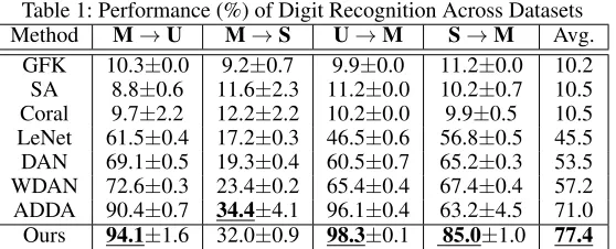
Table 1: Performance (%) of Digit Recognition Across Datasets

Method M→U M→S U→M S→M Avg.

GFK 10.3±0.0 9.2±0.7 9.9±0.0 11.2±0.0 10.2

SA 8.8±0.6 11.6±2.3 11.2±0.0 10.2±0.7 10.5

Coral 9.7±2.2 12.2±2.2 10.2±0.0 9.9±0.5 10.5

LeNet 61.5±0.4 17.2±0.3 46.5±0.6 56.8±0.5 45.5

DAN 69.1±0.5 19.3±0.4 60.5±0.7 65.2±0.3 53.5

WDAN 72.6±0.3 23.4±0.2 65.4±0.4 67.4±0.4 57.2

ADDA 90.4±0.7 34.4±4.1 96.1±0.4 63.2±4.5 71.0

Ours 94.1±1.6 32.0±0.9 98.3±0.1 85.0±1.0 77.4

Table 2: Performance (%) of Object Recognition Across Datasets onOffice-10+Caltech-10Dataset

Method D→C W→C A→C C→D C→W C→A Avg.

GFK 36.4±0.0 26.4±0.0 41.4±0.0 42.0±0.0 43.7±0.0 56.2±0.0 41.0

SA 34.4±0.0 32.3±0.0 40.6±0.0 43.7±0.0 40.6±0.0 45.4±0.0 39.5

Coral 33.8±0.0 33.8±0.0 45.1±0.0 45.9±0.0 46.4±0.0 52.1±0.0 42.8

LeNet 61.2±3.6 60.5±2.2 74.6±2.1 77.7±2.2 69.9±5.1 86.6±1.4 71.8

ADDA (LeNet) 74.7±3.9 75.9±2.9 78.4±1.5 28.0±5.1 47.1±5.3 77.7±3.5 66.0

Ours (LeNet) 80.6±0.0 81.7±0.0 82.7±0.1 81.4±0.7 80.0±0.2 91.2±0.1 82.9

AlexNet 80.8±0.4 76.1±0.5 83.8±0.3 89.0±0.3 83.1±0.3 91.1±0.2 84.0

DDC (AlexNet) 80.5±0.2 76.9±0.4 84.3±0.5 89.1±0.3 85.5±0.3 91.3±0.3 84.6

DAN (AlexNet) 82.0±0.4 81.5±0.3 86.0±0.5 90.5±0.1 92.0±0.4 92.0±0.3 87.3

Ours (AlexNet) 85.8±0.1 85.6±0.2 86.8±0.4 91.6±0.4 89.1±0.5 92.7±0.2 88.6

Gradients for θD and θC Equations (9) and (10) are

derivable, becauseLnD andLeC are typical cross-entropy losses, andLe_Dt is a quadratic loss. Thus, the gradients for

θDandθCcan be obtained by simply computing the deriva-tives of∂LnD/∂θDand∂(LeC +Le_Dt)/∂θC, respectively. The formulations are not detailed presented in this paper due to the limited space.

Gradient forθs The gradients ofLnM andLeC forθsin

Equation (7) can also be computed by derivation. On the other hand, Le_Ds in Equation (7) is a formulation based on the pair-wise similarityE_fij

s. This formulation causes a complexity of O(n2), where n is the number of source data. However, the complexity ofO(n2_{)is undesirable in}

deep-learning networks learned from large-scale datasets. Inspired by the unbiased estimation (Gretton et al. 2012), we adopt the strategy of sub-sampling without replacement to reduce the complexity ofLe_Ds toO(n). In particular, the unbiased estimator forLeDs is written as

2

n

n/2

X

i (1_[ya

s=ybs]ku i fs k

2

2 + 1[ya

s6=ybs]k`−u i fs k

2 2) (11)

whereui

fs = E

ab

fs = exp(−

za_s(z_sb)0

kza skkzsbk

), a = 2i−1 and

b= 2i. In deep-learning networks, normalization losses are used for source featuresza

s andzbs, and therefore,uifs can be approximated asui

fs = exp(−Ms(xas)(Ms(xbs))0). In the mini-batch SGD, we only need to consider the gra-dient with respect to each ui_f

s, so that we only introduce

the computation of gradient forLe_Ds(uifs). The gradient of Le_Ds can then be calculated by the combination of the gra-dients from eachui_f

s. We have

∂Le_Ds(uifs)

∂θs

=∂LeDs(u i fs)

ui fs

∂ui_f

s

∂θs

= 2(ui_f

s−1[yas6=ysb]`)

∂ui fs

∂θs

(12)

In summary, the gradient forθsin Equation (7) is the sum-mation of the gradients ofLnM,LeC andLeDs.

Gradient for θt Similarly, unbiased estimation (Gretton

et al. 2012) is adopted to reduce the complexity ofLeT in Equation (8). We write unbiased estimator forLeT as

2

n

n/2

X

i

(k H(ui_f

t, µft)− H(u i

t, µt)k22) (13)

whereui

ft =E

ab

ft ≈exp(−Mt(xat)(Mt(xbt))0),uit =Etab,

a= 2i−1andb= 2i. For eachui

fs, we have

∂LeT(uift,u i t)

∂θt

=∂LeT(u i ft)

∂B

∂B ∂ui ft

∂ui_ft

∂θt

= 2(B− H(ui_t, µt))B(1−B)

∂ui ft

∂θt (14)

whereB =H(ui ft, µft).

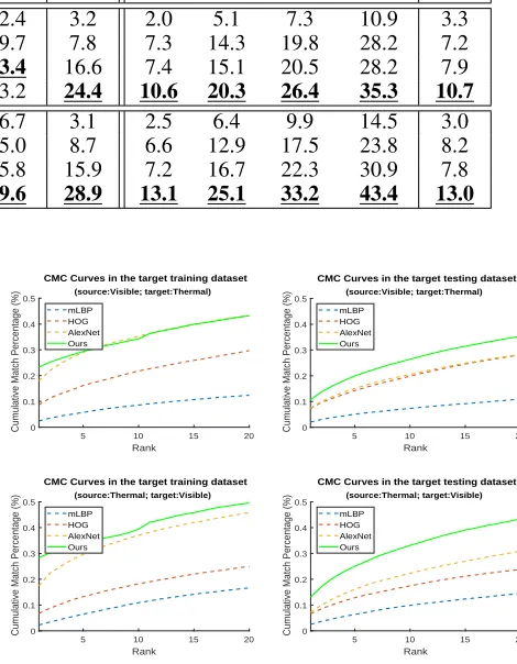
Table 3: Performance (%) of Cross-modal Person Re-identification on RegDB Dataset

Dataset Method Target-domain Training Dataset Target-domain Testing Dataset

r = 1 r = 5 r = 10 r = 20 mAP r = 1 r = 5 r = 10 r = 20 mAP

Visible→Thermal

mLBP 2.5 5.8 8.6 12.4 3.2 2.0 5.1 7.3 10.9 3.3

HOG 8.7 16.2 21.8 29.7 7.8 7.3 14.3 19.8 28.2 7.2

AlexNet 18.0 27.3 35.3 43.4 16.6 7.4 15.1 20.5 28.2 7.9

Ours 23.4 29.4 34.3 43.2 24.4 10.6 20.3 26.4 35.3 10.7

Thermal→Visible

mLBP 2.3 6.5 10.9 16.7 3.1 2.5 6.4 9.9 14.5 3.0

HOG 6.8 13.3 18.3 25.0 8.7 6.6 12.9 17.5 23.8 8.2

AlexNet 17.5 29.6 37.1 45.8 15.9 7.2 16.7 22.3 30.9 7.8

Ours 28.4 33.9 39.5 49.6 28.9 13.1 25.1 33.2 43.4 13.0

4

Experimental Results

In this section, we evaluate the proposed method on cross-dataset digit and object recognition. Evaluations are also performed on cross-modal re-identification. For each pair of datasets, experiments are conducted 10 times, and the aver-aged results in the target domains are reported. In Section 4.4, we visualize the aligned source and target features to further analyze the performance of the proposed unsuper-vised graph alignment method.

4.1

Cross-dataset Digit Recognition

Experiments of cross-dataset digit recognition are done across the full training set of three benchmarks (MNIST (Le-Cun et al. 1998), USPS and SVHN (Netzer et al. 2011) datasets). Ten classes of digits are contained in each dataset. In short, charactersM,UandSare used to represent MNIST, USPS, and SVHN datasets, respectively. Four adaptation di-rections (i.e.,M→U,M→S,U→M, andS→M) are used for evaluation. Following the network settings in (Tzeng et al. 2017), the source and target CNNs are implemented with the LeNet (LeCun et al. 1998), and the domain discrimina-tor is implemented with three fully connected layers: two layers with 500 hidden units followed by the final discrimi-nator output. Results are compared with statistical measure alignment methods (DAN (Long et al. 2015), WDAN (Yan et al. 2017), Coral (Sun, Feng, and Saenko 2016)), subspace alignment methods (GFK (Gong et al. 2012), SA (Fernando et al. 2013)), and ADDA (Tzeng et al. 2017) that learned the domain-indistinguishable features.

As shown in Table 1, the proposed method performs well among these four digit recognition experiments. The av-eraged accuracy of the proposed method is77.4%, which is the highest among all unsupervised domain adaptation methods. We achieve more than6%improvement over the second-best result. The proposed method also achieves the best results in the datasets ofM→ U,U→M, andS →

M. However, our result in theM→Sdataset is not as good as that of other datasets. This may be because the SVHN dataset is not well segmented, resulting in extensive noises contained in the structural information. These noises can spread to the aligned features via the consistency loss in the proposed adversarial network. Consequently, the recog-nition accuracy in the SVHN dataset is relatively low, but we

5 10 15 20

Rank

0 0.1 0.2 0.3 0.4 0.5

Cumulative Match Percentage (%)

CMC Curves in the target training dataset (source:Visible; target:Thermal) mLBP

HOG AlexNet Ours

5 10 15 20

Rank

0 0.1 0.2 0.3 0.4 0.5

Cumulative Match Percentage (%)

CMC Curves in the target testing dataset (source:Visible; target:Thermal) mLBP

HOG AlexNet Ours

5 10 15 20

Rank

0 0.1 0.2 0.3 0.4 0.5

Cumulative Match Percentage (%)

CMC Curves in the target training dataset (source:Thermal; target:Visible) mLBP

HOG AlexNet Ours

5 10 15 20

Rank

0 0.1 0.2 0.3 0.4 0.5

Cumulative Match Percentage (%)

CMC Curves in the target testing dataset (source:Thermal; target:Visible) mLBP

HOG AlexNet Ours

Figure 3: Cumulated matching characteristics (CMC) curves

still obtain the second best result inM→Sdataset.

4.2

Cross-dataset Object Recognition

Cross-dataset object recognition experiments are conducted across the Office-10 and Caltech-10 (Gong et al. 2012) datasets. In theOffice-10dataset, 10 classes (e.g., bike, bag, keyboard) of object images are captured from three differ-ent conditions: theAmazondataset consists of images down-loaded from websites, and theDslrandWebcamdatasets in-clude images taken by SLR and web cameras, respectively. Ten common categories of images that are shared with the

Office-10dataset are extracted from theCaltech-256dataset

to form theCaltech-10dataset. In Table 2, characterA,D,

WandCare used as the abbreviations to representAmazon,

Dslr, Webcam, and Caltech-10 datasets, respectively. Six

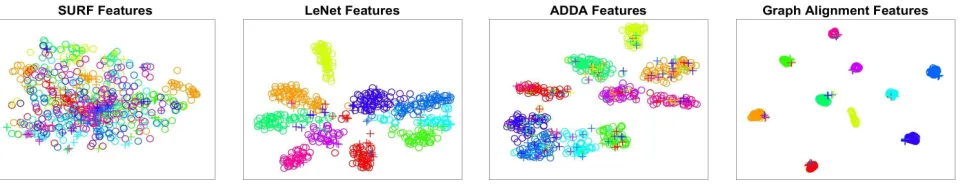
Figure 4: Spacial distributions of source (C) and target (D) features (◦: source-domain samples;+: target-domain samples)

2015))) domain adaptation methods. As discussed in (Long et al. 2015), features extracted by the lower convolutional layers are general. Thus, we initialize the AlexNet using the pre-trained ImageNet and only update the last three layers for adaptation. The implementation of domain discriminator is the same as that introduced in Section 4.1.

Table 2 presents the results of object recognition across

theOffice-10+Caltech-10datasets. It is shown that the

pro-posed method improves the recognition performance in the target domain by11.1% and4.6% with LeNet and AlexNet, respectively. Our method also outperforms other LeNet-based and AlexNet-LeNet-based unsupervised domain adaptation methods in almost all (expect one) datasets. We obtain an average accuracy of 82.9% and 88.6% with LeNet and AlexNet, respectively, which are the best results in Table 2.

4.3

Cross-modal Re-identification

The graph-aligned representations are validated across modality on RegDB (Nguyen et al. 2017) dataset that con-tains images of 412 persons captured by dual camera sys-tems. Two sub datasets are included in RegDB dataset: 1) Visible dataset with 10 visible light images of each per-son, and 2) Thermal dataset with 10 different thermal im-ages of each person. Following the experimental protocol in (Ye et al. 2018), we randomly split the Visible and Ther-mal datasets into two halves for training and testing. In the training phase, training images from one modality with la-bels (source domain) and the training images from the other modality without labels (target domain) are used. For test-ing, images in the target domain are used as the probe set while images in the source domain with the other modality as the gallery set. The verifications are performed on both target-domain training and testing datasets. To indicate the performance, the standard cumulated matching characteris-tics (CMC) curves are plotted in Figure 3, and mean average precision (mAP) is listed in Table 3.

As shown in Table 3, the deep-learning (AlexNet) features obtain better performance than the hand-craft features (HOG (Dalal and Triggs 2005) and mLBP (Moore and Bowden 2011)) in the target-domain training dataset. But the per-formance of AlexNet features in the target-domain testing dataset is as poor as the HOG and mLBP features. In con-trast, the proposed method achieves the highest average pre-cision in both training and testing datasets in the target do-main, which shows the better generalization ability of the proposed graph-aligned representations. Moreover, it is

dis-played in Figure 3 that the proposed method gets the highest matching scores at almost all ranks compared to other meth-ods in each experiment.

4.4

Visualization

In this section, we visualize graph-aligned representations in the source and target domains to qualitatively show the per-formance of the proposed method. T-SNE (Maaten and Hin-ton 2008) is employed, and the dataset ofC→Dis selected for visualization. SURF (Bay, Tuytelaars, and Van Gool 2006) features, features extracted from LeNet (LeCun et al. 1998) and ADDA (Tzeng et al. 2017) are also shown in Fig-ure 4 for comparison. Symbols◦and+are used to mark the features from source and target domains, respectively. Fea-tures of different classes are presented in different colors.

As shown in Figure 4, samples fromCaltech-10(source) and Dslr(target) datasets are disorderly distributed in the SURF feature space. This indicates that the hand-crafted fea-tures of SURF are not strongly discriminative toward class labels in both theCaltech-10andDslrdatasets. On the other hand, LeNet features are learned from source images and their labels, and therefore the source-domain LeNet features are more distinguishable for the class labels. But the dis-crimination is not extended to the Dslr dataset (target do-main), as the distributions of LeNet features from Caltech-10andDslrdatasets are not nicely matched. Compared to LeNet features, the marginal distributions of ADDA features from the Caltech-10 and Dslr datasets are better aligned. However, it can be found that each target sample is arbi-trarily aligned to one cluster of source samples. In addi-tion, some samples from different categories are closely dis-tributed in the ADDA feature space, which results in a diffi-culty of classification for samples from these classes.

fea-ture space. Therefore, the graph-aligned feafea-tures from the Dslrdataset are more discriminative toward class labels.

5

Conclusion

This paper proposes an unsupervised graph alignment method to address the problem of structural difference be-tween the source and target distributions in unsupervised do-main adaptation. An adversarial network is developed to ex-plore the cross-domain visual representations with losses of the node and edge alignments. Unified criteria are designed for edge alignment and used as loss functions for propaga-tion in the adversarial network. Experimental results show that the proposed method achieves promising results in the tasks of cross-domain recognition and re-identification.

Acknowledgments

This work was partially supported by the Science Faculty Research Grant of Hong Kong Baptist University, Hong Kong Research Grants Council General Research Fund:

RGC/HKBU12200518.

References

Bay, H.; Tuytelaars, T.; and Van Gool, L. 2006. Surf: Speeded up robust features. InECCV.

Chen, Q.; Liu, Y.; Wang, Z.; Wassell, I.; and Chetty, K. 2018. Re-weighted adversarial adaptation network for un-supervised domain adaptation. InCVPR.

Dalal, N., and Triggs, B. 2005. Histograms of oriented gra-dients for human detection. InIEEE Computer Society

Con-ference on Computer Vision and Pattern Recognition.

Fernando, B.; Habrard, A.; Sebban, M.; and Tuytelaars, T. 2013. Unsupervised visual domain adaptation using sub-space alignment. InICCV.

Ganin, Y.; Ustinova, E.; Ajakan, H.; Germain, P.; Larochelle, H.; Laviolette, F.; Marchand, M.; and Lempitsky, V. 2016. Domain-adversarial training of neural networks.JMLR. Gong, B.; Shi, Y.; Sha, F.; and Grauman, K. 2012. Geodesic flow kernel for unsupervised domain adaptation. InCVPR. Gong, B.; Grauman, K.; and Sha, F. 2013. Connecting the dots with landmarks: Discriminatively learning domain-invariant features for unsupervised domain adaptation. In

ICML.

Gopalan, R.; Li, R.; and Chellappa, R. 2011. Domain adap-tation for object recognition: An unsupervised approach. In

ICCV.

Gretton, A.; Borgwardt, K. M.; Rasch, M.; Sch¨olkopf, B.; and Smola, A. J. 2007. A kernel method for the two-sample-problem. InNIPS.

Gretton, A.; Borgwardt, K. M.; Rasch, M. J.; Sch¨olkopf, B.; and Smola, A. 2012. A kernel two-sample test. JMLR. Hou, C.-A.; Tsai, Y.-H. H.; Yeh, Y.-R.; and Wang, Y.-C. F. 2016. Unsupervised domain adaptation with label and struc-tural consistency. IEEE Transactions on Image Processing. Hu, L.; Kan, M.; Shan, S.; and Chen, X. 2018. Duplex gen-erative adversarial network for unsupervised domain adap-tation. InCVPR.

Krizhevsky, A.; Sutskever, I.; and Hinton, G. 2012. Im-agenet classification with deep convolutional neural net-works. InNIPS.

LeCun, Y.; Bottou, L.; Bengio, Y.; and Haffner, P. 1998. Gradient-based learning applied to document recognition.

Proceedings of the IEEE.

Long, M.; Ding, G.; Wang, J.; Sun, J.; Guo, Y.; and Philip, S. Y. 2013. Transfer sparse coding for robust image repre-sentation. InCVPR.

Long, M.; Wang, J.; Ding, G.; Shen, D.; and Yang, Q. 2014a. Transfer learning with graph co-regularization. TKDE. Long, M.; Wang, J.; Ding, G.; Sun, J.; and Yu, P. S. 2014b. Transfer joint matching for unsupervised domain adaptation. InCVPR.

Long, M.; Cao, Y.; Wang, J.; and Jordan, M. 2015. Learn-ing transferable features with deep adaptation networks. In

ICML.

Maaten, L. v. d., and Hinton, G. 2008. Visualizing data using t-sne. JMLR.

Moore, S., and Bowden, R. 2011. Local binary patterns for multi-view facial expression recognition. CVIU.

Netzer, Y.; Wang, T.; Coates, A.; Bissacco, A.; Wu, B.; and Ng, A. Y. 2011. Reading digits in natural images with un-supervised feature learning. InNIPS workshop.

Nguyen, D.; Hong, H. G.; Kim, K. W.; and Park, K. R. 2017. Person recognition system based on a combination of body images from visible light and thermal cameras. Sensors. Ni, J.; Qiu, Q.; and Chellappa, R. 2013. Subspace interpola-tion via dicinterpola-tionary learning for unsupervised domain adap-tation. InCVPR.

Sun, B., and Saenko, K. 2015. Subspace distribution align-ment for unsupervised domain adaptation. InBMVC. Sun, B., and Saenko, K. 2016. Deep coral: Correlation align-ment for deep domain adaptation. InECCV.

Sun, B.; Feng, J.; and Saenko, K. 2016. Return of frustrat-ingly easy domain adaptation. InAAAI.

Tenenbaum, J. B.; De Silva, V.; and Langford, J. C. 2000. A global geometric framework for nonlinear dimensionality reduction. science.

Tzeng, E.; Hoffman, J.; Zhang, N.; Saenko, K.; and Darrell, T. 2014. Deep domain confusion: Maximizing for domain invariance. arXiv preprint arXiv:1412.3474.

Tzeng, E.; Hoffman, J.; Saenko, K.; and Darrell, T. 2017. Adversarial discriminative domain adaptation. InCVPR. Wang, C., and Mahadevan, S. 2013. Manifold alignment preserving global geometry. InIJCAI.

Yan, H.; Ding, Y.; Li, P.; Wang, Q.; Xu, Y.; and Zuo, W. 2017. Mind the class weight bias: Weighted maximum mean discrepancy for unsupervised domain adaptation. InCVPR. Yang, B.; Ma, J.; and Yuen, P. 2018. Domain-shared group-sparse dictionary learning for unsupervised domain adapta-tion. InAAAI.