An Efficient Two Step Algorithm for High Dimensional
Change Point Regression Models Without Grid Search
Abhishek Kaul [email protected]
Department of Mathematics and Statistics Washington State University
Pullman, WA 99164, USA.
Venkata K. Jandhyala [email protected]
Department of Mathematics and Statistics Washington State University
Pullman, WA 99164, USA.
Stergios B. Fotopoulos [email protected]
Department of Finance and Management Science Washington State University
Pullman, WA 99164, USA.
Editor:Ryan Tibshirani
Abstract
We propose a two step algorithm based on`1/`0 regularization for the detection and
esti-mation of parameters of a high dimensional change point regression model and provide the corresponding rates of convergence for the change point as well as the regression parameter estimates. Importantly, the computational cost of our estimator is only 2·Lasso(n, p), where Lasso(n, p) represents the computational burden of one Lasso optimization in a model of size (n, p). In comparison, existing grid search based approaches to this problem require a computational cost of at least n·Lasso(n, p) optimizations. Additionally, the proposed method is shown to be able to consistently detect the case of ‘no change’, i.e., where no finite change point exists in the model. We allow the true change point parameterτ0 to possibly
move to the boundaries of its parametric space, and the jump sizekβ0−γ0k2 to possibly
diverge asnincreases. We then characterize the corresponding effects on the rates of con-vergence of the change point and regression estimates. In particular, we show that, while an increasing jump size may have a beneficial effect on the change point estimate, however the optimal rate of regression parameter estimates are preserved only upto a certain rate of the increasing jump size. This behavior in the rate of regression parameter estimates is unique to high dimensional change point regression models only. Simulations are per-formed to empirically evaluate performance of the proposed estimators. The methodology is applied to community level socio-economic data of the U.S., collected from the 1990 U.S. census and other sources.
Keywords: Change point regression, High dimensional models,`1, `0regularization, Rate
of convergence, Two phase regression
c
1. Introduction
Regression models are fundamental to supervised learning and statistical modelling of data collected from scientific phenomena. While applying regression models, one often assumes the regression parameters to be stable over time. However, this assumption may be rigid and may not hold in several environmental, biological and economic models, particularly when data is collected over an extended period of time. There are several approaches to model this dynamic phenomenon in regression parameters. One approach is to let the parameters change at certain unknown time points of the sampling period (Hinkley (1970), Hinkley (1972), Jandhyala and MacNeill (1997), Bai (1997), Jandhyala and Fotopoulos (1999), Fo-topoulos et al. (2010) and Jandhyala et al. (2013)). Another closely related approach is to formulate the change point based on one or more covariate thresholds (Hinkley (1969), Koul and Qian (2002) and Koul et al. (2003)). In the literature, it is common to broadly call both as change point regression models. Such dynamic models have been found to have wide ranging applications in all areas of scientific inquiry (Reeves et al. (2007), Lund et al. (2007), and Liu et al. (2013)).
Technological advances in the past two decades have led to the wide availability of large scale/high dimensional data sets in several areas of applications such as genomics, social networking, empirical economics, finance etc. This has led to rapid development of high dimensional statistical methods. A large body of literature has now been developed pertaining to the study of regression models capable of allowing a vastly larger number of parameterspthan the sample sizen.One of the most successful methods for analysing high dimensional regression models is the Lasso, which is based on the least squares loss and`1 regularization (Tibshirani (1996)). Innumerable investigations have since been carried out to study the behavior of the Lasso estimator and its various modifications in many different settings (see e.g., Zou (2006), Zhao and Yu (2006), Bickel et al. (2009), Belloni et al. (2011), Belloni et al. (2017a), Kaul (2014), Kaul and Koul (2015), and the references therein). For a general overview on the developments of Lasso and its variants we refer to the monograph of B¨uhlmann and Van De Geer (2011) and the review article of Tibshirani (2011). All aforementioned articles provide results in a regression setting where the parameters are dynamically stable. In the recent past, work has also been carried out in the context of high dimensional change point models in an ‘only means’ setup, where change occurs in only the mean of time ordered independent random vectors, with the dimension of the observation vector being larger than the number of observations (Cho and Fryzlewicz (2015), Fryzlewicz (2014), and Wang and Samworth (2018) among others). Here the change is characterized in the sense of a dynamic mean vector. Another context in which high dimensional change point models have been investigated is that of a dynamic covariance structure which is related to the study of evolving networks (Gibberd and Roy (2017), and Atchade and Bybee (2017)). In contrast, change point methods for high dimensional linear regression models have received much less attention and only a select few articles have considered this problem in the recent literature (Ciuperca (2014), Zhang et al. (2015), Leonardi and B¨uhlmann (2016), Lee et al. (2016), and Lee et al. (2018)).
In this paper, we consider a high dimensional linear regression model with a potential change point,
The observed variables in model (1.1) are,yi ∈R,thep-dimensional predictorsxi∈Rp,and change inducing variable wi ∈R, i = 1, .., n. The unknown parameters of interest are the regression parametersβ0, γ0∈Rp,and the change pointτ0 ∈R¯? :=R∪ {−∞}.The change point τ0 represents a threshold value of the variable w subsequent to which the regression parameter changes from its initial value β0 to a new value γ0.Note that, the ‘no change’ case is allowed by the model (1.1), since we allow τ0 = −∞, in its parametric space. In this case, model (1.1) reduces to an ordinary high dimensional linear regression model. The parametric space ¯R? of τ is restricted to only contain−∞,and not∞,since both of these points characterize the ‘no change’ scenario and are unidentifiable from each other. This differs from the usual characterization of the ‘no change’ case, which is typically defined by β0 =γ0 and τ0 ∈R,for e.g. in Lee et al. (2016) and Lee et al. (2018). However it should be understood that this difference is only notational and both are characterizing the same null model. It should also be noted that the change point τ0 ∈R¯∗, may itself depend on
n, i.e., as the sample size increases, the change point may shift its location. However, for clarity of exposition, this dependence is notionally suppressed in the rest of this article. Furthermore, we letp >> n,so that model (1.1) corresponds to a high dimensional setting. Also, consistent with current literature, we assume that only a total ofscomponents of β0 and γ0 are non-zero, i.e.,kβ0k0+kγ0k0≤s,where s < n.
Recently, models similar to (1.1) have been studied by Ciuperca (2014), Zhang et al. (2015), Leonardi and B¨uhlmann (2016), Lee et al. (2016) and Lee et al. (2018). Similar to model (1.1), Lee et al. (2016) and Lee et al. (2018) consider a high dimensional model with only a single unknown change point, whereas, Zhang et al. (2015), and Leonardi and B¨uhlmann (2016) consider a model where multiple change points may be present in the model. The articles Zhang et al. (2015) and Ciuperca (2014) consider a multiple change point setting where the dimension p of the regression parameters is fixed. The common thread in these articles is to provide regularized estimators for the parameters β, γ, τ and study their rates of convergence under different norms. In an earlier work, Wu (2008) provided an information-based criterion for carrying out change point analysis and variable selection in the fixed p setting; this methodology, however is not extendable to the high dimensional case. While these articles make important contributions to this fast emerging area, many aspects of this problem remain to be understood. For example, existing methods may be unable to satisfactorily detect the ‘no change’ case, these estimation methods may be computationally challenging to implement, and the underlying technical assumptions required for their theoretical validity may be restrictive.
The most commonly applied approach to estimating parameters of models such as (1.1) with a single change point is to consider,
( ˆβ,ˆγ,ˆτ) = arg min
β,γ∈Rp,τ∈T (
1 n
n X
i=1
loss(data, β, γ, τ) + pen(β, γ, τ)
)
, (1.2)
where loss(data, β, γ, τ) is an appropriately chosen loss function, and pen(β, γ, τ) is a suit-ably defined penalty function on the parameters β, γ, τ e.g., Lee et al. (2016), Lee et al. (2018) and (5.1)
is usually broken into a grid of points T∗, and ˆβ(τ),γˆ(τ) are computed for each τ ∈ T∗.
The estimate ˆτ of the change point τ0 is then obtained as thatτ ∈ T∗ which minimizes the objective function in (1.2) over ˆβ(τ),γˆ(τ).When the loss function is least squares and the penalty is of an`1-type, the computational cost of the above grid search is |T∗|Lasso(n, p), where|T∗|is typically of ordern. Note that this grid search mechanism becomes computa-tionally intensive asn, pincrease. In the case of multiple change points, Zhang et al. (2015), and Leonardi and B¨uhlmann (2016) provide dynamic programming approaches that can es-timate the number and locations of change points with the samenLasso(n, p) computational cost.
In this article we develop a two step algorithm for detection and estimation of parameters of model (1.1), so that a full grid search is avoided even as the near optimal rates of all parameter estimates are preserved. The idea for developing such an algorithm originates from the following simple and yet surprising numerical observation. Suppose we first choose virtually any initial valueτ(0) ∈Supp(w),separated from its boundaries and then compute regression coefficients ˆβ(0), γˆ(0) on the binary partition i;i ∈ {1, .., n}, wi ≤ τ(0) and
i;i∈ {1, .., n}, wi > τ(0) respectively. Then a single update of the change point estimate
obtained by optimization of the least squares loss over the change point parameter, using the previously obtained regression parameter estimates ˆβ(0),γˆ(0),yields a very precise estimate of the unknown change point, where the precision of this estimate is indistinguishable from existing full grid search approaches in any uniform sense. This simple numerical observation is very surprising, since it suggests that any initial τ(0) which carries even a ‘fractional amount of information’ on the unknown τ0 (this notion is described precisely later in Section 2), can be utilized to obtain an updated estimate ˆτ(1) in a single step, which lies in a near optimal neighborhood of τ0. In other words, the single step update process pulls in the initial guessτ(0) from a much wider (nearly arbitrary) neighborhood of τ0,to a near optimal neighborhood ofτ0.The usefulness of this process is immediate, as it removes the necessity of a grid search. The main contribution of this article is to develop a mathematical treatment of this two step algorithm. In doing so we also allow the possibility of ‘no change’ in the model (1.1).
More precisely, in this article we propose estimators based on `1/`0 regularization for the parametersτ0, β0,andγ0of model (1.1). The proposed methodology completely avoids a grid search approach for locating the unknown change point, consequently has a com-putational cost of only 2Lasso(n, p), significantly below the nLasso(n, p) cost of existing methods. A second important novelty of the proposed method, is its ability to detect the ‘no change’ case, which is achieved by a `0 regularization in the change point estimator. From a technical perspective, the rates of convergence associated with the proposed estima-tors are such that they are optimal for the regression parameter estimates and match the best rate of convergence available in the literature for estimating the change point. Before we describe our proposed methodology in Section 2, we outline below the notations used in this paper.
Notation: Throughout the paper, for any vector δ ∈Rp,kδk0 represents the number of non-zero components in δ.The normskδk1 and kδk2 represent the standard 1-norm and Euclidean norm, respectively. The normkδk∞ represents the sup norm, i.e., the maximum
of absolute values of all elements. For any set of indices T ⊆ {1, ...., p},let δT = (δj)j∈T
we let |T| represent the cardinality of the set T. The notation 1[·] represents the usual indicator function. We denote bya∧b= min{a, b},anda∨b= max{a, b},for anya, b∈R. In the following, let Supp(w) represent the support of the distribution ofwand Φ(·) be its cdf. Also denote by Φmin(τ0) = Φ(τ0)∧(1−Φ(τ0)).We shall use the following notation to represent generic constants that may be different from one term to the next. For example, 0< cu <∞ represent universal constants, whereas 0< cm <∞ are constants that depend
on model parameters such as variance parameters of underlying distributions. The generic constants 0< c1, c2 <∞are used to denote constants that may depend on bothcu,andcm.
Lastly, we shall denote by ¯R? :=R∪ {−∞},as the extended Euclidean space with negative infinity included. In the following, without loss of generality we assume that Supp(w) =R.
2. Methodology and Related Work
We begin this section by describing the proposed methodology for the detection and esti-mation of parameters of model (1.1). For this purpose we require the following notation. Let for anyτ ∈R¯?, β, γ ∈
Rp,
Q(τ, β, γ) = 1 n
n X
i=1
(yi−xTi β)21[wi ≤τ] +
1 n
n X
i=1
(yi−xTi γ)21[wi> τ].a (2.1)
Additionally define the following Condition I that shall serve as an initializing condition required for the construction of our proposed algorithm.
Condition I: Letu(0)n be a non-negative sequence defined as, u(0)n = 1∧cu
slogp
nl2
n 1
k
, for any constants, k∈[1,∞), andcu >0,b (2.2)
where 0 < ln ≤ 1/2 is any non-negative sequence. Then, assume that the initializer τ(0)
satisfies,
Φmin(τ(0))≥culn, and |Φ(τ(0))−Φ(τ0)| ≤u(0)n . (2.3)
In the above Condition I, the sequence ln and the constant k are arbitrary, subject to
satisfying Condition A(iii) to follow. The rate of the sequenceln shall control the ability of
Algorithm 1 to detect a finite change point near the boundaries ofR.Specifically Algorithm 1 shall be able to detect a finite change point (when it exists), such that Φmin(τ0) is of order at least that ofln.In the case where it is assumed that, either Φ(τ0) = 0 or Φmin(τ0)≥cu >0,
then we can set ln ≥ cu. Here, Algorithm 1 will be able to distinguish between the two
cases, whether (a) there is no change point, Φ(τ0) = 0 or (b) there is a finite change point τ0 ∈R such that Φ(τ0) is bounded below.c
Then, the two step algorithm which we propose to obtain change point and regression coefficient estimates is described in Algorithm 1 below.
a. Here, define1[wi≤τ] = 0,forτ =−∞.
b. Note here that the constantkis arbitrary, hence it can itself depend on initialτ(0),i.e., the farther the guessτ(0) is fromτ0 the largerkcan be chosen in order to satisfy Condition I.
Algorithm 1: Detection and estimation of change point and regression parameters
Step 0 (Initialize): Choose any initial valueτ(0)∈Rsatisfying Condition I. Compute the initial regression parameter estimates,
ˆ
β(0),γˆ(0)= arg min
β,γ∈Rp
n
Q(τ(0), β, γ) +λ1k(βT, γT)Tk1
o
, λ1 >0. Step 1: Updateτ(0) to obtain the change point estimate ˆτ(1) whered,
ˆ
τ(1) = arg min
τ∈R¯?
n
Q(τ,βˆ(0),ˆγ(0)) +µkΦ(τ)k0
o
, µ >0. (2.4)
Step 2: Update ( ˆβ(0),γˆ(0)) to obtain regression parameter estimates ( ˆβ(1),ˆγ(1)) where, ˆ
β(1),γˆ(1)
= arg min
β,γ∈Rp
n
Q(ˆτ(1), β, γ) +λ2k(βT, γT)Tk1
o
, λ2 >0.
A first concern that may arise to reader regarding Step 0 of Algorithm 1 pertains to the initializing conditions in (2.3) of Condition I. The first of these conditions is clearly innocuous, all it requires is the initial user chosen τ(0) to be marginally away from the boundaries of R. The second condition in (2.3) requires that the initial value τ(0) be in an u(0)n -neighborhood of τ0. While at first, this might come across as a limitation of the algorithm, however the following discussion shall show how broad this u(0)n -neighborhood
truly can be. First note that the constantk∈[1,∞) is arbitrarily large, subject to Condition A(iii), i.e., this condition is adaptable to the user chosen value of the initializerτ(0).In other words, the farther the user chosenτ(0) is from the true change pointτ0,the larger the value of k can be, in order to satisfy this condition. Additionally, note that the largest possible distance (in the cdf scale) between any twoτ1, τ2 ∈R,is such that|Φ(τ1)−Φ(τ2)| ≤1.Now forcu= 1,consider first the disallowed case ofk=∞,then the initial condition is trivially
satisfied, since |Φ(τ(0))−Φ(τ0)| ≤ 1. Thus, virtually any initial value in the parametric space of τ0, separated from its boundaries, will satisfy the required initial condition for a large enough k∈[1,∞), thereby illustrating that this initial condition is infact very mild. Remarkably, one of our main results shows that, under suitable conditions, the updated change point estimate ˆτ(1) of Step 1 of Algorithm 1, will satisfy optimal error bounds, irrespective of the value of k. Simply stated, the update in Step 1 sharpens the initial change point guess from any arbitrary fractional rate to a near optimal rate. The condition (2.3), also provides a precise description of the notion of ‘fractional information’ mentioned in the introduction section. The sequence u(0)n forms a metric measuring the amount of
information in the guess τ(0) about τ0,and the existence of a finite k <∞ provides a way of saying that the guessτ(0) possesses some fractional amount of information on τ0.
To numerically illustrate this surprising phenomenon, in Section 5 we use the ‘no in-formation’ initializer τ(0) = w(0.5), i.e. the 50th percentile of w.e Note that this choice is
d. Note that while the initializing τ(0) inStep 0 is chosen in
R, however the optimization inStep 1 is
performed over the extended Euclidean space ¯R?=R∪ {−∞}.
the most sensible value of the initializer in the absence of any information about τ0.These numerical results provide strong evidence to support Algorithm 1 by showing that the pre-cision of the estimates obtained from the proposed method are infact indistinguishable from existing grid search type approaches, and are obtained with a small fraction of the com-putational burden. Another equivalent way of viewing the above discussion is that, if we pick two distinct initializers τ1(0) and τ2(0) carrying some fractional information about τ0, i.e., they satisfy the initializing condition for some 1 ≤k1 < k2 < ∞, respectively (τ1(0) is closer to τ0 than τ2(0)), then, the corresponding updated change point estimates ˆτ
(1) 1 , τˆ
(1) 2 will both be in a near optimal neighborhood ofτ0.This basically implies that the quality of the guess does not influence the updated estimate in its eventual rate of convergence. This observation is also numerically illustrated in Section 5.
Finally, we also mention that a slight relaxation of Condition I is also possible, specifi-cally, the sequence u(0)n in this condition can instead be relaxed to u(0)n = 1∧cu(1n)1/k,for
any constants k ∈[1,∞) and anycu >0,while preserving all results to follow. However,
Condition I in its current form provides a coherence with other noise bounds that show up in the statement and proof of our results, and thus is a notationally convenient representa-tion. Furthermore, this relaxation of Condition I shall not yield error bounds that are any sharper than those to follow.
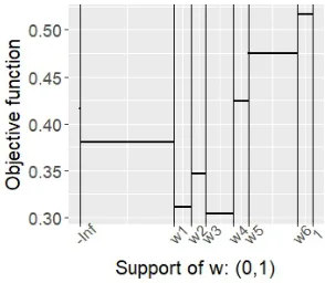
A second concern that may arise to the reader regarding implementation of Algorithm 1 is the feasibility of implementing Step 1. At first, this optimization seems intractable owing to its nonsmooth, nonconvex (with no apparent convex relaxations) construction. However, upon closer inspection, it is observed that the loss function Q(·,βˆ(0),γˆ(0)) in Step 1 is a step function with step changes occurring at any point on the one-dimensional grid (−∞, w1, w2, ..., wn)T.Secondly, the `0 term in the objective function only depends on whether Φ(τ) is zero or non zero. This implies that the distance between any twoτ1 and τ2 does not influence the value of the`0 norm (note that this will not be the case if instead an `1 norm is used). These two observations together imply that any global optimum achieved in the extended Euclidean space ¯R? will also be attained at some point on the finite grid (−∞, w1, w2, ..., wn)T.An illustration of this step behavior is provided in Figure 1.
A final concern in implementing Step 1 is that it requires knowledge of the distri-bution function Φ(·), which is typically unknown. This concern is also easily overcome upon observing that the objective function in Step 1 is a step function over the grid (−∞, w1, w2, ..., wn)T.Specifically, on this grid, the term kΦ(τ)k0=kτk∗0,where kτk∗0 = 1, ifτ ∈ {w1, ..., wn} and kτk∗0 = 0,ifτ =−∞.
In view of the above discussion,Step 1of Algorithm 1 can be replaced by the following optimization,
ˆ
τ(1) = arg min
τ∈{−∞}∪{w1,...,wn}
n
Q(τ,βˆ(0),γˆ(0)) +µkτk∗0o, µ >0. (2.5)
Figure 1: Step behavior of the functionQ(·,β,ˆ ˆγ) +µkΦ(τ)k0,withµ= 0.1,evaluated over grid of points
{−∞}∪{0,0.01, ...,1}.Herewi∼ U(0,1), n= 6, τ0= 0.25, p= 3, β0= (1,0,0)T, γ0= (0,1,0)T,
and we use ˆβ= (0.41,0,0)T,ˆγ= (0.13,0.92,0)T.The realizations{w1, .., wn}have been sorted (ascending) in the illustration. Observe that step changes occur at−{∞} ∪ {w1, w2, ..., wn}.
Another note of interest is the convenience of separability in computing the optimizers ˆ
β,γˆ inStep 0and Step 2, i.e., for any fixedτ,we can obtain
ˆ
β(τ) = arg min
β∈Rp
n1
n
X
i;wi≤τ
(yi−xTi β)2+λ1kβk1
o
, (2.6)
ˆ
γ(τ) = arg min
β∈Rp
n1
n
X
i;wi>τ
(yi−xTi γ)2+λ1kγk1
o
. (2.7)
These are ordinary Lasso optimizations and can be carried out by any one of the several methods available in the literature. Some of these methods include, coordinate or gradient descent algorithms (see, e.g. Hastie et al. (2015)), or via interior point methods for linear optimization under second order conic constraints (see, e.g., Koenker and Mizera (2014)).
The main results of this article establish selection consistency of the unknown change point and provide finite sample bounds for the error in estimates obtained from Algorithm 1 under suitable conditions. Let ξn := kβ0 −γ0k2 be the jump size between the pre and post regression parameters. Then the specific results we derive are,
(i) If Φ(τ0) = 0, then Φ(ˆτ(1)) = 0, (2.8) (ii) If Φmin(τ0)≥culn, then|Φ(ˆτ(1))−Φ(τ0)| ≤tn:=cucmmax
nslogp
n , 1 (1∨ξ2
n)l2n slogp
n
o
,
(iii) βˆ(1)−β0
q ≤cucms
1/q 1
Φmin(τ0)max
n r
logp n , ξntn
o
, q= 1,2,
(iv) ˆγ(1)−γ0
q≤cucms
1/q 1
Φmin(τ0)max
n r
logp n , ξntn
o
, q = 1,2,
with probability at least 1−c1exp(−c2logp),fornsufficiently large.
the following special case. Upon letting ξns p
logp/n → 0, and ln ≥ cu, in (2.8), the last
three results of (2.8) reduce to,
(i) If Φmin(τ0)≥culn, then|Φ(ˆτ(1))−Φ(τ0)| ≤cucm slogp
n , (2.9)
(ii) βˆ(1)−β0
q ≤cucms 1
q
r
logp
n , q= 1,2,
(iii) ˆγ(1)−γ0
q≤cucms 1
q
r
logp
n , q= 1,2,
with probability at least 1−c1exp(−c2logp),fornsufficiently large.
In an ordinary high dimensional linear regression model without change points, it has been shown that the optimal rate of convergence for regression estimates ispslogp/n un-der the `2 norm (see, e.g.,Ye and Zhang (2010), Raskutti et al. (2011), and Belloni et al. (2017b)). This implies that the rate of convergence of the regression estimates from Algo-rithm 1 (which stops after one iteration) cannot be uniformly improved upon by carrying out further iterations (over subgaussian distributions). Also, the rate of convergence of the change point estimate in (2.9) is the fastest available rate in the literature. We shall now state the conditions under which the results of this article are derived.
Condition A (assumptions on model parameters):
(i) Let S = S1 ∪S2, where S1 = {j;β0j 6= 0} and S2 = {j;γ0j 6= 0}. Then for some s=sn≥1,we assume that|S| ≤s.
(ii) The model dimensions s, p, n, satisfy slogpn → 0. Additionally, the sequence ln of
Condition I satisfiesslogpnl2n→0.
(iii) If a finite change point exists, i.e., Φmin(τ0) > 0, then the sequence ln and constant k∈[1,∞) of Condition I satisfy
s l2
n
slogp
nl2
n 1k
→0.
Additionally, in this case Φmin(τ0)≥culn.
(iv) If Φmin(τ0) > 0,then the jump size is bounded below by a constant, i.e, ξn := kβ0− γ0k2> c >0.
Condition B (assumptions on model distributions):
(i) The vectors xi = (xi1, ..., xip)T, i = 1, .., n, are i.i.d subgaussianf with mean vector
zero, and variance parameterσ2x≤C.Furthermore, the covariance matrix Σ :=ExixTi has
bounded eigenvalues, i.e., 0< κ≤mineigen(Σ)<maxeigen(Σ)≤φ <∞.
(ii) The errorsεi’s are i.i.d. subgaussian with mean zero and variance parameter σε2≤C.
(iii) The variableswi, i= 1, ..., nare i.i.d r.v.’s (continuous or discrete), with its cdf Φ(a) = P(wi≤a), a∈R.
f. Recall that forα >0,the random variableηis said to beα-subgaussian if, for allt∈R, E[exp(tη)]≤
exp(α2t2/2).Similarly, a random vectorξ∈Rpis said to beα-subgaussian if the inner productshξ, vi
(iv) The r.v.’sxi, wi, εi are independent of each other.
Conditions A(i) and A(ii) together form the usual sparsity assumption of high dimen-sional models. Conditions A(ii) and A(iii) are both restrictions on the model dimensions and in fact A(ii) is implied by A(iii) when it is applicable. However, both conditions are stated here since some of our results in Sections 3 and 4, hold under the weaker Condition A(ii). The Condition A(iii) is on the model parameters and also related to the initial condi-tion of Condicondi-tion I, via the sequencelnand the constantk∈[1,∞).This condition assumes
the only additional control on how large a constantkand how small the sequenceln,can be
tolerated by Algorithm 1, given the model dimensions. Heuristically, this condition ensures that the fractional information possessed by the initial guess τ(0),is not dominated by the noise induced in the linear system due to its large dimensions. Note that Condition A(iii) is only assumed if a change point exists, i.e., Φmin(τ0) > 0. In the case of ‘no change’ in model (1.1), i.e., Φ(τ0) = 0, any initial value τ(0) satisfying Φ(τ(0)) ≥culn, i.e., separated
from the boundaries of R, can be used to initialize Algorithm 1. A secondary purpose that Condition A(iii) serves is to ensure that if a finite change point exists, then, to keep Φmin(τ0) ≥culn away from the boundaries of (0,1),whenever a finite change point exists
in the model. Note that, this condition does not assume lower boundedness of Φmin(τ0) as is commonly the case in the literature, since the sequenceln may converge to zero. Finally,
Condition A(iv) requires that if a finite change point exists, then the corresponding jump sizeξn is bounded below. We also mention here that we do not make any assumptions on
the upper bound ofξn,and this jump size is allowed to possibly diverge withn.
The subgaussian assumptions in Conditions B(i) and B(ii) are now standard in high dimensional linear regression models and are known to accommodate a large class of random designs. In ordinary high dimensional linear regression, these assumptions are used to establish well behaved restricted eigenvalues of the Gram matrixP
xixTi /n(Raskutti et al.
(2010), and Rudelson and Zhou (2012)), which are in turn used to derive convergence rates of`1 regularized estimators (Bickel et al. (2009), and several others). These conditions play a similar role in our change point setup.
One main advantage of the proposed Algorithm 1 over existing methods is its ability to provide near optimal estimates without a grid search. As mentioned earlier in the article, the computational cost of Algorithm 1 is 2Lasso(n, p), significantly below the nLasso(n, p) cost of existing methods and is thus scalable to deal with large data. A novelty of Algorithm 1 in comparison to those proposed in Leonardi and B¨uhlmann (2016), Lee et al. (2016) and Lee et al. (2018) is its ability to detect the case where Φ(τ0) = 0.This is relevant since it removes the necessity to pre-test for the existence of a change point. In contrast, while the methods of Lee et al. (2016), and Lee et al. (2018) are implementable in the case of no change point, they are however unable to detect the absence of the change point. Instead, in this case of Φ(τ0) = 0,these methods return a valid 2p dimensional estimate (ˆγT,αˆT)T,where α0 = β0−γ0,that can be used for predictive purposes using the model (1.1). Note that, the ability to detect the absence of a change point is a stronger statement and may provide additional relevant information, while also preserving the interpretablepdimensional linear regression model in the case where Φ(τ0) = 0.
given in Appendix A, while Appendix B consists of some relevant auxiliary results from the literature, stated without proofs. The performance of Algorithm 1 is empirically evaluated in Section 5. In this numerical section, the implementation of Algorithm 1 assumes no prior information of the unknown change point τ0, additionally we numerically illustrate that the quality of the initial guess has no discernible impact on the final estimates and finally, we also show that the precision of the proposed estimates is indistinguishable from grid search approaches. Section 6 consists of an application of the proposed methodology to socio-economic data of U.S. collected from the 1990 U.S. census, and other sources.
3. Preliminary Results
In this section we present preliminary results that are important for stating and proving our main results in Section 4. First, for any fixedτ, we define
ζi(τ) = (
1[τ0< wi ≤τ], if τ > τ0 1[τ ≤wi < τ0], if τ ≤τ0.
Then clearly, for any fixed τ ∈R, Eζi(τ) := Φ∗(τ0, τ) =|Φ(τ)−Φ(τ0)|.We shall now state a key result that uniformly controls (over τ) the quantityn−1Pn
i=1ζi(τ).
Lemma 3.1 Let un, and vn be any non-negative sequences such that vn ≥clogp/n, c >0 and letT(τ0, un) =
τ : Φ∗(τ0, τ)≤un be aun-neighborhood ofτ0.Then under Condition
B(iii), we have,
(i) sup
τ∈T(τ0,un)
1 n
n X
i=1
ζi(τ)≤cumax nlogp
n , un
o
, (ii) inf
τ∈R; Φ∗(τ0,τ)≥vn
1 n
n X
i=1
ζi(τ)≥cuvn,
with probability at least 1−c1exp(−c2logp).
To proceed further, define for any τ the following set of random indices,
nw :=nw(τ0, τ) =
(
i∈ {1, ..., n}; τ0< wi ≤τ, if τ ≥τ0, i∈ {1, ..., n}; τ ≤wi < τ0, if τ ≤τ0.
(3.1)
Note that the cardinality of the random setnw is precisely the stochastic term controlled in
Lemma 3.1, i.e., |nw|=Pin=1ζi(τ).This relation serves to provide bounds on several other
stochastic terms considered in subsequent lemmas. The relationship between the cardinality of the random index setnw and the r.v.’sζi(τ), i= 1, ..., nhas also been used by Kaul et al.
(2017) in the context of graphical models with missing data.
Then under Condition B, we have for any fixed δ ∈Rp that,
(i) sup
τ∈T(τ0,un)
1 n
X
i∈nw
δTxixTi
∞≤cucm1kδk2max nlogp
n , un
o
,
(ii) sup
τ∈T(τ0,un)
1 n
X
i∈nw
δTxixTi δ≤cucm1kδk22max
nlogp
n , un
o
,
(iii) sup
τ∈T(τ0,un)
1 n
X
i∈nw εixTi
∞≤cucm2 r
logp n max
n r
logp n ,
√ un
o
,
with probability at least 1 −c1exp(−c2logp). Here cu > 0 is a universal constant, and cm1 = (φ+σx+σx2), cm2 = (
√
σεσx+σεσx) are model constants.
Finally in order to obtain the desired error bounds (2.8) and (2.9) we require re-stricted eigenvalue conditions on the gram matrix Pn
i=1xixTi . For any deterministic set S ⊂ {1,2, ..., p},define the collectionA as,
A=
n
δ∈Rp;kδSck1 ≤3kδSk1,
o
. (3.2)
Then, Bickel et al. (2009) define the lower restricted eigenvalue condition as,
inf
δ∈A
1 n
n X
i=1
δTxixTi δ ≥cuκkδk22, for some constantκ >0. (3.3)
Other slightly weaker versions of this condition are also available in the literature such as the compatibility condition of B¨uhlmann and Van De Geer (2011), and the `q sensitivity
of Gautier and Tsybakov (2011). In the setup of common random designs, it is also well established that condition (3.3) holds with probability converging to 1,see for e.g. Raskutti et al. (2010), and Rudelson and Zhou (2012), for Gaussian designs. In the subgaussian case, the plausibility of this condition is a consequence of a general result stated as Lemma B.2 in Appendix B. Under our high dimensional change point setup, we shall require versions of the restricted eigenvalue condition (3.3). In the following lemma, we shall show that all required conditions hold with probability converging to 1.Among other arguments, the proof of these conditions shall rely on Lemma B.2. In Lemma 3.3 below, the collection A in (3.2) applies for the set S in Condition A.
Lemma 3.3 (Restricted Eigenvalue Conditions): Let un, and vn be any non-negative se-quences such that vn ≥clogp/n, c > 0. Let T(τ0, un) be as in Lemma 3.1 and the set A
as defined in (3.2) for S given in Condition A. Furthermore, define the set A2 =
n
δ ∈
Rp;kδSck1≤3kδSk1+ 3kβ0−γ0k1
o
,and let anyτ ∈Rbe such that Φ−min1 (τ)slogp/n=o(1).
re-stricted eigenvalue conditions hold with probability at least 1−c1exp(−c2logp), (i) inf
δ∈A
1 n
X
i;wi≤τ
δTxixTi δ≥cuκΦ(τ)kδk22,
(ii) inf
δ∈A
1 n
X
i;wi>τ
δTxixTi δ≥cuκ(1−Φ(τ))kδk22,
(iii) sup
τ∈T(τ0,un)
sup
δ∈A
1 n
X
i∈nw
δTxixTi δ≤cucmkδk22max
nslogp
n , un
o
,
(iv) inf
τ∈R; Φ∗(τ0,τ)≥vn
inf
δ∈A2
1 n
X
i∈nw
δTxixTi δ ≥cucmvnkδk22−cucm slogp
n
kδk22+ξ2n
.
Before moving on to state our main results in the next section, we make the following remark regarding the role of the setA2.
Remark 3.1 Note that if β −β0 ∈ A, i.e., kβSc −β0Sck1 ≤ 3kβS−β0Sk1, then for δ = β0−γ0+β−β0,we have,
kδSck1≤ kβSc−β0Sck1 ≤3kβS−β0Sk1 ≤3kδSk1+ 3kβ0−γ0k1.
Thus β−β0 ∈ A,implies the vector δ ∈A2.This relation is useful in proving Lemma 4.1 and Theorem 4.2 of the next section.
4. Main Results
We are now ready to state our first main result pertaining to the rate of convergence of the regression estimates obtained from (2.6) and (2.7) when τ(possibly random) is in a un-neighborhood of τ0.
Theorem 4.1 Suppose Conditions A(i), A(ii), and B hold, and consider any τ ∈R, satis-fying Φ−min1 (τ)slogp/n=o(1). Let βˆ(τ) andγˆ(τ) be solutions to (2.6) and (2.7). Then, (i) When Φ(τ0) = 0 and λ1≥cucm
p
logp/n, for nsufficiently large, we have for q= 1,2,
kβˆ(τ)−γ0kq≤cucm
1 Φmin(τ)
s1/q
r
logp n ,
with probability at least1−c1exp(−c2logp).The same bound holds forkγˆ(τ)−γ0kq, q = 1,2. (ii) When Φmin(τ0) >0, let un be any non-negative sequence satisfying un =o Φmin(τ0)
.
Also, letT(τ0, un) be as defined in Lemma 3.1 andλ1=cucmmax{ p
logp/n, ξnun}.Then for n sufficiently large, and q= 1,2,the following uniform bound holds,
sup
τ∈T(τ0,un)
kβˆ(τ)−β0kq≤cucm
1 Φmin(τ0)s
1/qmaxn r
logp
n ,kβ0−γ0k2un
o
,
Remark 4.1 As a direct consequence of Theorem 4.1, we obtain the rates of convergence of the regression estimates ˆβ(0),γˆ(0) from Step 0of Algorithm 1. Specifically, under the conditions of Theorem 4.1,
(i) When Φmin(τ0) = 0,
kβˆ(0)−γ0kq≤cucm
1 Φmin(τ(0))s
1/q r
logp
n , q= 1,2,
with probability at least 1 −c1exp(−c2logp). The same bound holds for kγˆ(0) −γ0kq, q= 1,2.
(ii) When Φmin(τ0)>0,and
Φ(τ
(0))−Φ(τ0) ≤u
(0)
n ,we have,
kβˆ(0)−β0kq ≤cucm
1 Φmin(τ0)s
1/qmaxn r
logp n , ξnu
(0)
n o
, q = 1,2,
(4.1)
with probability at least 1−c1exp(−c2logp).The same bound holds forkˆγ(0)−γ0kq, q= 1,2.
In this case, sinces1/qξnu(0)n .
Φ(τ0) may diverge, these estimates are not guaranteed to be consistent. Nevertheless, (i) and (ii) above play an important role in deriving convergence rates of estimators from subsequent steps of Algorithm 1.
We now turn our attention to establishing selection and estimation results for estimates obtained from Step 1 and Step 2 of Algorithm 1. To achieve this goal, we require the following notations. For any τ ∈R, β, γ ∈Rp,let
Rn(τ, β, γ) = Q(τ, β, γ)−Q(τ0, β, γ).
Sn(τ, β, γ) = Rn(τ, β, γ) +µ kΦ(τ)k0− kΦ(τ0)k0
Also, for any non-negative un,andvn,define the collection
H(un, vn) =
τ ∈R; vn≤ |Φ(τ)−Φ(τ0)| ≤un
Additionally, for any non-negative sequence un,we also define the function,
F(un) = (
0 if un
Φmin(τ0)→0
1 otherwise . (4.2)
Finally, in the following, we denote by rn:= max p
slogp/n,√sξnun(0) Φmin(τ0), in the case where Φmin(τ0)>0.Notice thatrnis the`2rate of estimation error provided in Part(ii) of Remark 4.1. The following lemma provides a uniform lower bound of the expression Sn(τ, β, γ),over the collectionH(un, vn),that holds with high probability. This result shall
lie at the heart of the argument used to obtain the main results of this article.
(i) When Φ(τ0) = 0, for anyvn>0,we have
inf
τ∈H(1,vn)Sn(τ, ˆ
β(0),γˆ(0))≥µ−cucm
slogp nΦ2
min(τ(0))
with probability at least 1−c1exp(−c2logp).
(ii) When Φmin(τ0)>0, for anyvn≥clogp/n, c >0,we have,
inf
τ∈H(un,vn)
Sn(τ,βˆ(0),ˆγ(0))≥ξ2n
cucmvn−cucm slogp
n −
cucm
1∨ξn r
slogp
n max
n r
logp n ,
√ un
o
−cucm rn2 1∨ξ2
n
max
nslogp
n , un
o
− cuµ
1∨ξ2
n F(un)
.
with probability at least 1−c1exp(−c2logp).
Our main result on rate of convergence of the estimates obtained from Algorithm 1 is stated in Theorem 4.2 below. While the complete proof of the theorem is given in the appendix, here we provide a sketch of the main idea behind the proof. We show that, for an appropriately chosen regularizer µ, for anyvn>0 (in the case where Φ(τ0) = 0), or for
any non-negative sequence vn slower in rate than those given in (2.8) (in the case where
Φmin(τ0)>0), we shall show that, inf
τ;vn≤Φ∗(τ0,τ)≤1
Sn τ,βˆ(0),γˆ(0)
>0, fornsufficiently large.
with probability at least 1−c1exp(−c2logp). Upon noting that the global optimizer ˆτ(1) by definition satisfies Sn(ˆτ(1),βˆ(0),γˆ(0))≤0,we would have shown that the corresponding
global optimizer ˆτ(1) satisfies the relations given in (2.8). Along the way a sequence of recursions are required in order to sequentially sharpen the bound for the change point estimate. Supportive arguments are also required to show that the eventual bound is satisfied with probability at least 1−c1exp(−c2logp).In this process, Remark .1 is quite helpful.
Theorem 4.2 Suppose Conditions A and B hold and chooseλ1=cucmmax{ p
logp/n, ξnu(0)n }, andµ=cucm slogp/nln2
1/k∗
,where k∗ = max{k,2}.Then for nsufficiently large, the op-timizer τˆ(1) of Step 1of Algorithm 1 satisfies the following relations.
(i) When Φ(τ0) = 0, thenΦ(ˆτ(1)) = 0,with probability at least 1−c1exp(−c2logp).
(ii) When Φmin(τ0)≥culn,then,
|Φ(ˆτ(1))−Φ(τ0)| ≤tn:=cucmmax
nslogp
n , 1 (1∨ξ2
n)l2n slogp
n
o
,
with probability at least 1−c1exp(−c2logp).
Theorem 4.3 Suppose the model (1.1) in the case where a finite change point exists, i.e.,
Φmin(τ0)>0.Assume the conditions of Theorem 4.2 and chooseλ2=cucmmax p
logp/n, ξntn , where tn is as defined in Theorem 4.2. Then, the estimatesβˆ(1) and γˆ(1) of Step 2 of Al-gorithm 1 satisfy,
(i) kβˆ(1)−β0kq≤cucms1/q
1
Φmin(τ0)max
n r
logp n , ξntn
o
, q= 1,2,
(ii) kγˆ(1)−γ0kq ≤cucms1/q
1 Φmin(τ0)
maxn
r
logp n , ξntn
o
, q = 1,2,
with probability at least 1−c1exp(−c2logp).
Remark 4.2 (Interpretation of the rates of Theorem 4.2 and Theorem 4.3) Note that under conditions of Theorem 4.2, and additionally assuming that ξnln ≥ c1 > 0, we have,
|Φ(ˆτ(1))−Φ(τ0)| ≤cucm slogp
n ,
with probability at least 1−c1exp(−c2logp).This observation provides an intuitive state-ment, saying that an increasing jump sizeξncan compensate for the location of the unknown
change point moving toward the boundaries of R, in effect allowing ˆτ(1) of Algorithm 1 to approximate the unknown change point (if it exists) at a near optimal rate. In this case, under conditions of Theorem 4.3, the regression estimates of Step 2become,
kβˆ(1)−β0kq≤cucms1/q
1
Φmin(τ0)max
n r
logp n , ξn
slogp n
o
, q = 1,2, (4.3)
with probability at least 1−c1exp(−c2logp).The same bound also holds for kˆγ(1)−γ0kq, q = 1,2,with the same probability. The bound in the statement (4.3) again provides an interesting observation, where an increasing jump is leading to potentially counteract the precision of the regression estimate ˆβ(1).First note that, the bound in (4.3) can tolerate an increasing jump sizeξnsuch thatξns
p
logp/n→0,while preserving optimality of the rate of convergence, i.e, yielding,kβˆ(1)−β0k2 ≤cucmΦ−1(τ0)
p
slogp/n, with high probability. It is only when ξn increases faster than
p
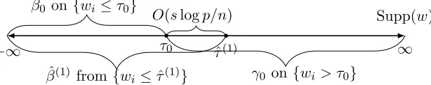
n/s2logp that it begins to harm the rate of convergence. This observation is surprising in that it suggests that an increasing jump size always benefits the change point estimate, whereas it benefits the regression coefficient estimates only when the jump size is increasing upto a certain rate. To the best of our knowledge, such a characterization of the effect of the jump size on parameter estimates, which holds only in the high dimensional case, has not been provided in the literature. The illustration in Figure 2 provides an intuitive understanding of this behavior,
−∞
Supp(w)
τ0 ˆτ(1) ∞
O(slogp/n)
ˆ
β(1) from {wi ≤τˆ(1)} γ0 on{wi > τ0} β0 on{wi ≤τ0}
From Figure 2, observe that for any finite jump size, the best approximation that our analysis can provide is wherein the error is of orderslogp/n.g Now the regression estimates ofStep 2are computed based on the binary partition yielded by the change point estimate ˆ
τ(1) of Step 1. Consequently, the data based on which the regression estimate ˆβ(1) of β0 is obtained, may be corrupted by as much as a fractionO(slogp/n) of observations where the true regression coefficient isγ0.Thereby, the higher the jump sizeξn,the more impact
this small corruption will have on the estimate ˆβ(1).The same argument also holds for the other binary partition. This provides an explanation of the rates observed in Theorem 4.3.
5. Implementation and Numerical Results
The three main objectives of this empirical study are, (i) to evaluate the overall performance of Algorithm 1, i.e., its ability to consistently estimateβ0, γ0,and a finite τ0,and compare its performance to a full grid search approach, (ii) to numerically support the theoretically claimed statement, that the estimate ˆτ(1) is insensitive to the quality of the initial guess τ(0), and (iii) to evaluate the numerical performance of Algorithm 1 in detecting the ‘no change’ case, i.e., when Φ(τ0) = 0.
5.1. Simulation setup
We consider the data generating process (1.1) whereεi, wi andxi are drawn independently
satisfying εi ∼ N(0, σε2), wi ∼ U(0,1),h and xi ∼ N(0,Σ). Here, Σ is a p×p matrix with
elements Σij =ρ|i−j|, i, j= 1, ..., p. We set,σε = 1 and ρ= 0.5.The regression parameters
of the model are set to beβ0 = (1,1,1,1, ...,0)Tp×1,andγ0 = (01×4,1,1,1,1,0, ...,0)Tp×1.The metrics of interest are bias and mean squared error of various estimates: For numerical experiments where Φmin(τ0)>0,bias( ˆβ) =kE( ˆβ−β0)k2, bias(ˆγ) =kE(ˆγ−γ0)k2, bias(ˆτ) =
|E(ˆτ −τ0)|, mse( ˆβ) = kE( ˆβ −β0)2k2, mse(ˆγ) = kE(ˆγ −γ0)2k2, mse(ˆτ) = E(ˆτ −τ0)2, mse(Φ(ˆτ)) = E(Φ(ˆτ)−Φ(τ0))2. For numerical experiments where Φ(τ0) = 0, we report P rM = E(1[ˆτ(1) = −∞]), i.e., the proportion of times where the ‘no change’ model is correctly identified. We shall report monte carlo approximations of these metrics based on 100 replications for each combination of model parameters. In the simulations where a finite change point, i.e., 0 < τ0 <1 is misidentified as ‘no change point’, i.e., ˆτ(1) =−∞,
observed to occur sometimes whenτ0 is near the boundaries of (0,1)
, we do the following operation to maintain fairness of comparisons of the above metrics. In case whereτ0 <0.5 and ˆτ(1)=−∞,then we set ˆτ(1) = 0,βˆ(1) = 0p×1,and whenτ0 >0.5 and ˆτ(1) =−∞,we set ˆ
τ(1) = 1,ˆγ(1) = 0p×1.Finally, we also report the metrictime: the average (over replications) computation timei. All computations are performed in the software R, R Core Team (2017). All lasso optimizations are performed with the R package ‘glmnet’, developed by Friedman et al. (2010). We perform two sets of simulations for all combinations of the parameters n ∈ {150,250,350}, p ∈ {25,150,250}. In the first simulation, we consider finite change points, with τ0 ∈ {0.169,0.264, ...,0.831}, (Equally spaced grid of 8 points between 0.169 to 0.831). This is referred to as Simulation A in the following. The second simulation considers the case of ‘no change’ in the model (1.1), i.e.,τ0 = 0.This simulation is referred
g. This rate matches the fastest available in the literature
h. Since wi∼ U(0,1),hence Φ(τ) =τ, τ ∈(0,1).
to as Simulation Bin the following. Due to the absence of any comparative method that is able to detect the ‘no change’ case (to the best of our knowledge), we report only the results of our method for this simulation. Note that for each fixed p, the total number of model parameters to be estimated is 2p+ 1.
Choice of tuning parameters: The regularizerλ1 andλ2 of the Lasso optimizations of Step 0 and Step 2 of Algorithm 1 are chosen via a 5-fold cross validation, which is performed internally by the R package ‘glmnet’. The regularizerµof Step 1of Algorithm 1 is chosen via the classical BIC criteria. Specifically, ˆτ(µ) is computed over a grid of values of µ.Then, the value of µof that minimizes the criteria,
BIC(µ) = logQ τˆ(µ),βˆ(µ),γˆ(µ)
+logn
n kΦ ˆτ(µ)
k0,
is chosen. Here Q(·,·,·) is the least squares loss, as defined in (2.1), and ˆβ(µ), γˆ(µ) represent regression coefficient estimates obtained on the binary partition given by ˆτ(µ).
In the following, we consider two schemes to choose the initializerτ(0) ofAlgorithm 1. The first is to set tow(0.5),i.e., the 0.5thempirical quantile ofw= (w1, .., wn)T.This is done
to make the initializer equidistant from the two extremes of the support ofw.Note that, in the absence of any information on the unknownτ0,the choiceτ(0) =w(0.5)is a sensible choice for the initializer. This approach is represented as ‘Algorithm 1A’. As a second scheme, we choose the initializer τ(0) by setting it to one of values {w(m); m = 0.25,0.50,0.75}, wherew(m) represents themth empirical quantile ofw= (w1, ..., wn)T.This is done by first
computing ˆβ(τ) and ˆγ(τ) in (2.6) and (2.7) for each τ =w(0.25), w(0.50), w(0.75),and finally selecting τ(0) as the value that minimizes the least squares loss over these three choices. Note that the latter approach has an additional computational burden of two Lasso(n, p) optimizations in comparison to the former. This approach is represented as ‘Algorithm 1B’. Clearly, the initializer in Algorithm 1B will be a closer value to the unknown τ0 in comparison to the initializer of Algorithm 1A. This shall also help us numerically support our theoretical finding that Algorithm 1 is insensitive to the ‘quality’ of the initializer. Finally, we also implement the full grid search approach of Lee et al. (2016) in order to serve as a benchmark to compare the performance of the proposed estimates and also to illustrate the dramatic gains in computation time provided by our method. This approach is referred to asFull grid searchin the following. For completeness, theFull grid search estimator of Lee et al. (2016) is described in the notation of this article in the following. The article of Lee et al. (2016) assumes the modelyi =xiδ0+xiTη01[wi ≤τ0],which is equivalent
to the model (1.1) whenδ0 =γ0 andη0 =β0−γ0.Now, let ˜xi(τ) = xTi , xTi1(wi ≤τ) T
2p×1, and the parameter α = (γ, β−γ), where β0, γ0 are the true parameter coefficients of the model (1.1), then
ˆ
α(τ) = arg min
α∈R2p
n1
n n X
i=1
(yi−x˜Ti (τ)α)2+λkD(τ)αk1
o
, for eachτ ∈ T∗,
ˆ
τ = arg min
τ∈T∗
n1
n n X
i=1
yi−x˜Ti (τ) ˆα(τ) 2
+λkD(τ) ˆα(τ)k1
o
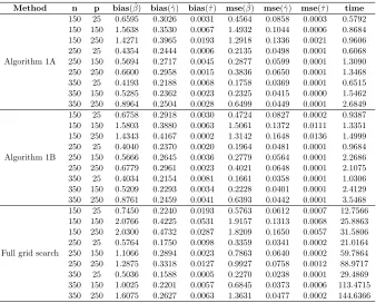
Table 1: Numerical results ofAlgorithm 1A and 1B, and Full grid searchforn ∈ {150,250,350}, p∈ {25,150,250},andτ0= 0.169.
Method n p bias( ˆβ) bias(ˆγ) bias(ˆτ) mse( ˆβ) mse(ˆγ) mse(ˆτ) time
Algorithm 1A
150 25 0.6595 0.3026 0.0031 0.4564 0.0858 0.0003 0.5792 150 150 1.5638 0.3530 0.0067 1.4932 0.1044 0.0006 0.8684 150 250 1.4271 0.3965 0.0193 1.2918 0.1336 0.0021 0.9606 250 25 0.4354 0.2444 0.0006 0.2135 0.0498 0.0001 0.6068 250 150 0.5694 0.2717 0.0045 0.2877 0.0599 0.0001 1.3090 250 250 0.6600 0.2958 0.0015 0.3836 0.0650 0.0001 1.3468 350 25 0.4193 0.2188 0.0068 0.1758 0.0369 0.0001 0.6515 350 150 0.5285 0.2362 0.0023 0.2325 0.0415 0.0000 1.5462 350 250 0.8964 0.2504 0.0028 0.6499 0.0449 0.0001 2.6849
Algorithm 1B
150 25 0.6758 0.2918 0.0030 0.4724 0.0827 0.0002 0.9387 150 150 1.5803 0.3880 0.0063 1.5061 0.1372 0.0111 1.3351 150 250 1.4343 0.4167 0.0002 1.3142 0.1648 0.0136 1.4999 250 25 0.4040 0.2370 0.0020 0.1964 0.0481 0.0001 0.9684 250 150 0.5666 0.2645 0.0036 0.2779 0.0564 0.0001 2.2686 250 250 0.6779 0.2961 0.0023 0.4021 0.0648 0.0001 2.1075 350 25 0.4034 0.2154 0.0081 0.1661 0.0358 0.0001 1.0306 350 150 0.5209 0.2293 0.0034 0.2228 0.0401 0.0001 2.4129 350 250 0.8761 0.2459 0.0041 0.6393 0.0442 0.0001 3.5468
Full grid search
150 25 0.7450 0.2240 0.0193 0.5763 0.0612 0.0007 12.7566 150 150 2.0766 0.4225 0.0531 1.9157 0.1313 0.0068 25.8863 150 250 2.0300 0.4732 0.0287 1.8209 0.1650 0.0057 31.5806 250 25 0.5764 0.1750 0.0098 0.3359 0.0341 0.0002 21.0164 250 150 1.1066 0.2894 0.0023 0.7863 0.0640 0.0002 59.7864 250 250 1.2875 0.3318 0.0127 0.9927 0.0758 0.0012 88.9717 350 25 0.5036 0.1588 0.0005 0.2270 0.0238 0.0001 29.4869 350 150 1.0025 0.2201 0.0057 0.6845 0.0373 0.0006 113.4715 350 250 1.6075 0.2627 0.0063 1.3631 0.0477 0.0002 144.6366
where D(τ) = diag
kx˜(j)(τ)kn, j = 1, ...,2p , with ˜x(j)(τ) representing the jth column of the design matrix ˜x(τ) = x˜1(τ), ...,x˜n(τ)
T
n×2p. In implementation of this estimator, the
search space of the change point is restricted toτ ∈ T∗ ={w1, ..., wn} ∩(0.1,0.9).
5.2. Results and discussion
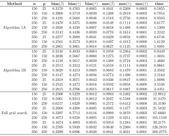
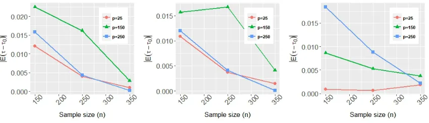
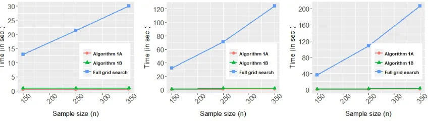
The bias and mean squared error (mse) of estimates obtained from Algorithms 1A, 1B, and Full grid search for Simulation A, for all combinations of n ∈ {150,200,250}, p ∈ {25,150,250}, and Φ(τ0) ∈ {0.169,0.67} are presented in Table 1 and Table 2. All results provided are truncated at 10−4.Complete results of the simulation study including all cases for τ0 ∈ {0.169,0.264, ...,0.831}, are available in the supplementary materials of this article. To aid in interpretation, the results on bias are illustrated through Figures 3, 4, 5, 6 and 7. In particular, Figure 3 illustrates bias associated with the change point estimate, Figure 4 and Figure 5 illustrate the bias in ˆβ(1),and ˆγ(1) respectively. In Figure 6 we illustrate the consistency of the proposed methodology and finally, in Figure 7 we depict the average computation time for the methods implemented in this simulation study. The results ofSimulation Bare reported in Table 3. This table reports the proportion of times the ‘no change’ model is correctly identified via the metricP rM as described above.
indis-Table 2: Numerical results ofAlgorithm 1A and 1B, and Full grid searchforn ∈ {150,250,350}, p∈ {25,150,250},andτ0= 0.642.
Method n p bias( ˆβ) bias(ˆγ) bias(ˆτ) mse( ˆβ) mse(ˆγ) mse(ˆτ) time
Algorithm 1A
150 25 0.3170 0.4765 0.0065 0.1041 0.2308 0.0003 0.5855 150 150 0.3900 0.5719 0.0039 0.1309 0.2819 0.0002 0.7854 150 250 0.4191 0.5668 0.0046 0.1510 0.2756 0.0004 0.8583 250 25 0.2470 0.3375 0.0088 0.0548 0.1114 0.0002 0.6177 250 150 0.2926 0.4248 0.0007 0.0658 0.1486 0.0001 1.1309 250 250 0.3142 0.4436 0.0039 0.0770 0.1614 0.0001 1.3242 350 25 0.2277 0.3098 0.0041 0.0429 0.0858 0.0001 0.6748 350 150 0.2501 0.3573 0.0018 0.0497 0.1012 0.0000 1.6129 350 250 0.2861 0.3861 0.0018 0.0627 0.1135 0.0001 1.8991
Algorithm 1B
150 25 0.3148 0.4833 0.0064 0.1059 0.2364 0.0002 0.9449 150 150 0.3826 0.5667 0.0060 0.1275 0.2737 0.0002 1.3024 150 250 0.4138 0.5617 0.0039 0.1489 0.2724 0.0004 1.4660 250 25 0.2512 0.3312 0.0121 0.0558 0.1114 0.0003 0.9661 250 150 0.3029 0.4213 0.0005 0.0683 0.1470 0.0001 2.3502 250 250 0.3147 0.4274 0.0056 0.0773 0.1490 0.0001 2.2163 350 25 0.2318 0.3071 0.0043 0.0436 0.0847 0.0001 1.0086 350 150 0.2525 0.3472 0.0016 0.0502 0.0958 0.0000 2.5538 350 250 0.2815 0.3766 0.0015 0.0617 0.1087 0.0000 3.4451
Full grid search
150 25 0.2506 0.5229 0.0012 0.0983 0.2482 0.0002 12.9812 150 150 0.5061 0.9313 0.0012 0.2037 0.5588 0.0009 31.2470 150 250 0.6217 1.0329 0.0065 0.2572 0.6412 0.0008 35.3190 250 25 0.2000 0.4208 0.0005 0.0505 0.1477 0.0003 21.5832 250 150 0.3397 0.7712 0.0116 0.0909 0.3870 0.0003 67.6660 250 250 0.4072 0.8228 0.0005 0.1229 0.4251 0.0001 105.1549 350 25 0.1674 0.4083 0.0045 0.0353 0.1284 0.0001 30.2175 350 150 0.2769 0.5949 0.0032 0.0640 0.2360 0.0001 126.2810 350 250 0.3299 0.6896 0.0030 0.0841 0.3031 0.0001 200.2775
Table 3: Numerical results ofSimulation B, where the underlying model isyi=xTiγ0+εi,i.e., the ‘no change’ case where Φ(τ0) = 0.The metricP rM is reported for each combination ofn, p.
n Algorithm 1A Algorithm 1B
p= 25 p= 150 p= 250 p= 25 p= 150 p= 250 150 0.76 0.87 0.88 0.76 0.87 0.88 250 0.80 0.93 0.91 0.80 0.93 0.91 350 0.85 0.93 0.94 0.85 0.93 0.94
Figure 3: Comparison of bias(ˆτ) forAlgorithm 1A and 1Band Full grid searchacross values of τ0
Figure 4: Comparison of bias( ˆβ) forAlgorithm 1A and 1B, andFull grid searchacross values ofτ0
forp= 250.Left panel: n= 150,Center panel: n= 250,Right panel: n= 350.
Figure 5: Comparison of bias(ˆγ) forAlgorithm 1A and 1B, andFull grid searchacross values ofτ0
forp= 250.Left panel: n= 150,Center panel: n= 250,Right panel: n= 350.
Figure 6: Illustration of consistency of implemented methods withτ0 = 0.264. Left panel: Algorithm
Figure 7: Comparison of computation time (in seconds) for Algorithm 1A and 1B, and Full grid searchacross values ofnforτ0= 0.547 Left panel: p= 25,Center panel:p= 150,Right panel:
p= 250.Note that, these times are computed as averages over 100 replications of each method running in parallel over 12 cores. Running a single instance of any method is two to three times faster. Reported computation times include time taken to choose tuning parameters.
tinguishable from the Full grid search approach of Lee et al. (2016). Second, it is also observed that the proposedAlgorithms 1A and 1Bare indistinguishable from each other in terms of the bias in the change point estimate. Recall that, Algorithm 1B was designed in a way so that the starting value is always closer to τ0 in comparison to Algorithm 1A. Despite a better initial value, no uniform improvement is observed in Algorithm 1B. This supports our theoretical result, that the quality of the initial value does not impact Algorithm 1, and it yields near optimal estimates with any initializing value containing any fractional information on the unknown change point. The bias results for the regression co-efficient estimates depicted in Figures 4 and Figure 5 suggest that the proposed methodology yields a uniformly lower bias at all considered cases of τ0.One possible reason for this be-havior is that the design variable in our methodology are constructed aszi= (zi(1)T, z
(2)T i )T
where zi(1) =xi1[wi ≤τ0], and zi(2) =xi1[wi ≤τ0], which are orthogonal to each other, in contrast, the design variables in the methodology of Lee et al. (2016), the design variables are constructed as z(1)i = xi and zi(2) = 1[wi ≤τ0], which may be highly correlated. It is also clear from Figure 6 that the in bias in change point estimates from Algorithm 1A and 1B and Full grid search progressively shrinks with increasing values of n, thereby illustrating the consistency of the proposed methodology. Finally, in Figure 7 we illustrate the dramatic differences in the overall computation times in the implementation of the com-pared approaches. In the largest considered data set, the average time for computation of Algorithm 1A and 1Bwas≈3seconds, as opposed to the full grid search which required
≈ 200seconds to implement. Note that the reported computation times include the time taken for choosing all required tuning parameters for each method.
Simulation B: The results of Simulation B reported in Table 3 are in accordance with expectations. The proposed methods are able to detect the ‘no change’ scenario with
1A and 1Bare seen to provide the exact same results, which is again not surprising since the only difference in these two methods is the choice of the initial value.
6. Application
In this section, we apply our proposed methodology to the ‘Communities and Crime’ data set of Redmond and Baveja (2002), available publicly athttps://archive.ics.uci.edu/ ml/datasets/Communities+and+Crime. This data contains: (i) socio-economic data at a community level from across the entire United states, and is collected from the 1990 US Census, (ii) law enforcement data from the 1990 US Law Enforcement Management and Administrative Statistics survey, and (iii) crime data from the 1995 FBI Uniform Crime. The full data set contains 1994 observations and 128 variables. The dependent variable of interest is the total number of violent crimes per one hundred thousand population, which is calculated using the population and the sum of the crime variables that are considered violent crimes: murder, rape, robbery, and assault. The remaining variables are quantitative measurements on socio-economic variables such as the median (community level) income per household, percentage of people aged 16 and over who are employed, percentage of households with public assistance, percent of population who have immigrated within the last 10 years, amongst many others. This data was recently analyzed by Leonardi and B¨uhlmann (2016) for detecting and identifying change points in covariates when the change point(s) are modeled over locations. In this study we are interested in identifying changes in covariates when the change occurs through a change inducing variable. Specifically, we consider tow cases, (1) when the change inducing variable is assumed to be the population for the community, and (2) when the change inducing variable is assumed to be the median household income for the community, in an effort to investigate whether violent crime at a community level is influenced by distinct socio-economic factors below and above a certain threshold of population or the median household income, and also to estimate the threshold level at which such a transition occurs.
The full data set consists of n = 1994 observations andp = 128 variables, which have been normalized to [0,1] scale. The normalization process is described in the webpage whose link has been provided at the beginning of this section. This normalized data is pre-processed by deleting observations with any missing values, and by eliminating predictors that are highly correlated with other predictor variables. After the pre-processing, we obtain a filtered data set with n = 319 communities. The remaining data is then mean centered and scaled columnwise in order to remove the need for an intercept term in the regression, mainly to be consistent with model (1.1). Finally, predictor variables having a significant correlation with the change inducing variable have also been dropped from the analysis. This process yields a refined data set withp= 75 predictor variables (excluding the change inducing variable) in the case where the change inducing variable is ‘population’ andp= 77 in the case where the change inducing variable is ‘median income’
Table 4: Summary of analysis of ‘Communities and Crime’ data set. Change inducing variable (w): pop-ulation, model size: n= 319, p= 75.Estimated change point is ˆτ(1) = 0.24,which is the 73rd percentile of the population variable. The table lists all estimated non-zero regression coefficients truncated at 10−4.
Variable Description Coefficient (βˆSˆ)
(pre change)
Coefficient (γˆSˆ) (post change) racepctblack % of population that is african american 0.0322 0.0000
racePctWhite % of population that is caucasian -0.1844 0.0000
pctWWage % of households with wage or salary income in 1989 -0.0505 0.0000 pctWInvInc % of households with investment / rent income in 1989 -0.0909 0.0000
PctPopUnderPov % of people under the poverty level 0.0686 0.0000
PctEmploy % of people 16 and over who are employed -0.0069 0.0000
PctIlleg % of kids born to never married 0.3105 0.1734
PctHousLess3BR % of housing units with less than 3 bedrooms 0.0199 0.0000
PctHousOccup % of housing occupied -0.0359 0.0000
PctVacantBoarded % of vacant housing that is boarded up 0.0000 0.0743
NumStreet # of homeless people counted in the street 0.0000 0.1597
LemasSwFTFieldOps # of sworn full time police officers in field operations 0.0000 -0.0229 PolicReqPerOffic total requests for police per police officer (0/1) 0.0229 0.0000
LemasGangUnitDeploy gang unit deployed 0.0196 0.0000
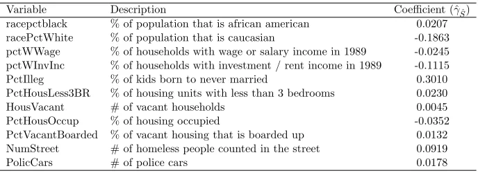
Table 5: Summary of analysis of ‘Communities and Crime’ data set. Change inducing variable (w): median income, model size: n = 319, p = 77. Estimated change point is ˆτ(1) = −∞,i.e., no change
detected in the model w.r.t. w. The table lists all estimated non-zero regression coefficients truncated at 10−4.
Variable Description Coefficient (ˆγSˆ)
racepctblack % of population that is african american 0.0207 racePctWhite % of population that is caucasian -0.1863 pctWWage % of households with wage or salary income in 1989 -0.0245 pctWInvInc % of households with investment / rent income in 1989 -0.1115
PctIlleg % of kids born to never married 0.3010
PctHousLess3BR % of housing units with less than 3 bedrooms 0.0230
HousVacant # of vacant households 0.0045
PctHousOccup % of housing occupied -0.0352
PctVacantBoarded % of vacant housing that is boarded up 0.0132 NumStreet # of homeless people counted in the street 0.0919
PolicCars # of police cars 0.0178
Acknowledgement
We thank three anonymous referee’s for insighfut comments and suggestions that led to a significant improvement to the results and presentation of the manuscript.
Appendix A: Proofs
Proof of Lemma 3.1: Let τ1 > τ0 be a boundary point on the right of τ0, such that Φ∗(τ0, τ1) =un.Then recall that
ζi(τ1) =1[τ0 < wi≤τ1], Φ∗(τ0, τ) = Φ(τ1)−Φ(τ0).
Also, note that pn:=Eζi(τ1) = Φ∗(τ0, τ1).Since ζi, i= 1, ..., n are Bernoulli r.v.’s, for any s > 0, the moment generating function is given by E(exp(sζi)) = qn+pnexp(s), where qn= 1−pn.Applying the Chernoff Inequality, we obtain,
P n X
i=1
ζi(τ1)> t+npn
=P ePni=1sζi(τ1)> e(st+snpn)≤e−s(t+npn)[q
n+pnes]n.
Now in order to show,
P1 n
n X
i=1
ζi(τ1)≤cumax nlogp
n , un
o
≥ 1−c1exp(−c2logp). (A.1) We divide the argument into two cases. First, for any arbitrary constant cu > 0, we let
Φ∗(τ0, τ1)≥culogp/n,upon choosing t=nΦ∗(τ0, τ1) we obtain, P
n X
i=1
ζi(τ1)>2nΦ∗(τ0, τ1)
≤e[−2snΦ∗(τ0,τ1)][1 + (Φ∗(τ
0, τ1))(es−1)]n.
Using the deterministic inequality (1 +x)k≤exp(kx),for any k, x >0,we obtain that
P n X
i=1
ζi(τ1)>2nΦ∗(τ0, τ1)
≤e−2snΦ∗(τ0,τ1)e(es−1)nΦ∗(τ0,τ1)≤e−c2logp.
The inequality to the right follows by choosing s = log 2, which maximizes the function f(s) = 2s−es+1 and provides a positive value at the maximum, and by using the restriction Φ∗(τ0, τ)≥culogp/n.Next we let Φ∗(τ0, τ1)< culogp/n.Here chooset=culogpto obtain, P
n X
i=1
ζi(τ1)> culogp+nΦ∗(τ0, τ1)
≤e[−sculogp−snΦ∗(τ0,τ1)][1 + (Φ∗(τ
0, τ1))(es−1)]n(A.2). Calling upon the inequality (1 +x)k≤exp(kx),for any k, x >0,we can bound the RHS of (A.2) from above by exp−sculogp+ (es−s−1) logp
.Now s= log(1 +cu) provides a
positive value at the maximum, since it maximizes f(s) = (1 +cu)s−es+ 1.Then for any cu >0,we obtain,
P n X
i=1
ζi(τ1)> culogp+nΦ∗(τ0, τ1)
Upon combining both cases, (A.1) follows by noting Φ?(τ0, τ1) =un.
Now repeating the same argument for a fixed boundary point τ2 on the left of τ0, such that Φ(τ0)−Φ(τ2) =un,and applying a union bound we obtain,
P
max
τ∈{τ1,τ2}
1 n
n X
i=1
ζi(τ)≤cumax nlogp
n , un
o
≥1−c1exp(−c2logp). (A.3)
It remains to show that (A.1) holds uniformly over T(τ0, un).For this, we begin by noting
that for any τ ∈ T(τ0, un),where τ > τ0 we have ζi(τ) =1
wi ∈(τ0, τ]
≤1wi∈(τ0, τ1]
. Similarly for any τ ∈ T(τ0, un) whereτ < τ0 we have ζi(τ)≤1
wi∈[τ2, τ0)
.Thus
sup
τ∈T(τ0,un)
1 n
n X
i=1
ζi(τ)≤ max τ∈{τ1,τ2}
1 n
n X
i=1
ζi(τ). (A.4)
Part (i) of this lemma follows by combining (A.4) with the bound in (A.3).
To prove Part (ii) we use a lower bound for sums of non-negative r.v.s’ stated in Lemma B.3. This result was originally proved by Maurer (2003). For a fixed right boundary point τ1 > τ0 such that Φ(τ1)−Φ(τ0) =vn,sett=vn/2 in Lemma B.3. Then we have
P1 n
n X
i=1
ζi(τ1)≤ vn
2
≤exp−nvn
≤c1exp(−c2logp),
where the last inequality follows fromvn≥culogp/n.We obtain the same bound applying
a similar argument for the left boundary pointτ2 < τ0 such that Φ(τ0)−Φ(τ2) =vn.Now
applying an elementary union bound we obtain
P min
τ∈{τ1,τ2}
1 n
n X
i=1
ζi(τ)≥cuvn
≥1−c1exp(−c2logp). (A.5)
Finally to obtain uniformity over τ ∈
τ; Φ∗(τ0, τ) ≥ vn note that for τ > τ0, we have ζi(τ) = 1
wi ∈ (τ0, τ]
≥ 1
wi ∈ (τ0, τ1]
and for any τ < τ0, we have ζi(τ) = 1
wi ∈
[τ, τ0)
≥1
wi ∈[τ2, τ0)
.This implies that
inf
{τ; Φ∗(τ
0,τ)≥vn} 1 n
n X
i=1
ζi(τ)≥ min τ∈{τ1,τ2}
1 n
n X
i=1
ζi(τ). (A.6)
Part(ii) follows by combining (A.5) and (A.6). This complete the proof of Lemma 3.1.
Proof of Lemma 3.2: We begin with the proof of Part (i). Note that the RHS of the inequality in Part (i) is normalized by the `2 norm of δ.Hence, without loss of generality we can assume kδk2 = 1. Now, the proof of this lemma relies on|nw|=Pni=1ζi(τ),where ζi(τ) are as defined for Lemma 3.1. Note that if |nw| = 0 then Lemma 3.2 holds trivially
with probability 1,thus without loss of generality we shall assume that |nw|>0.Now, for
any fixedτ ∈ T(τ0, un),we have 1 n X
i∈nw
δTxixTi ∞≤
|nw| n
1
|nw| X
i∈nw
δTxixTi