Bayesian Network Learning via Topological Order
Young Woong Park [email protected]
College of Business Iowa State University Ames, IA 50011, USA
Diego Klabjan [email protected]
Department of Industrial Engineering and Management Sciences Northwestern University
Evanston, IL 60208, USA
Editor:Zhihua Zhang
Abstract
We propose a mixed integer programming (MIP) model and iterative algorithms based on topological orders to solve optimization problems with acyclic constraints on a directed graph. The proposed MIP model has a significantly lower number of constraints compared to popular MIP models based on cycle elimination constraints and triangular inequalities. The proposed iterative algorithms use gradient descent and iterative reordering approaches, respectively, for searching topological orders. A computational experiment is presented for the Gaussian Bayesian network learning problem, an optimization problem minimizing the sum of squared errors of regression models with L1 penalty over a feature network with application of gene network inference in bioinformatics.
Keywords: Bayesian networks, topological orders, Gaussian Bayesian network, directed acyclic graphs
1. Introduction
Directed graphGis a directed acyclic graph (DAG) or acyclic digraph ifGdoes not contain a directed cycle. In this paper, we consider a generic optimization problem over a directed graph with acyclic constraints, which require the selected subgraph to be a DAG.
Let us consider a complete digraph G. Let m be the number of nodes in digraph G,
Y ∈Rm×m a decision variable matrix associated with the arcs, where Y
jk is related to arc
(j, k), supp(Y) ∈ {0,1}m×m the 0-1 (adjacency) matrix with supp(Y)
jk = 1 if Yjk 6= 0,
supp(Y)jk = 0 otherwise,G(supp(Y)) the sub-graph ofGdefined bysupp(Y), and letAbe
the collection of all acyclic subgraphs ofG. Then, we can write the optimization problem with acyclic constraints as
min
Y F(Y) s.t. G(supp(Y))∈ A, (1)
whereF is a function ofY.
Acyclic constraints (or DAG constraints) appear in many network structured problems. The maximum acyclic subgraph problem (MAS) is to find a subgraph ofGwith maximum cardinality while the subgraph satisfies acyclic constraints. MAS can be written in the
c
form of (1) with F(Y) = −ksupp(Y)k0. Although exact algorithms were proposed for a superclass of cubic graphs (Fernau and Raible, 2008) and for general directed graphs (Kaas, 1981), most of the works have focused on approximations (Even et al., 1998; Hassin and Rubinstein, 1994) or inapproximability (Guruswami et al., 2008) of either MAS or the minimum feedback arc set problem (FAS). FAS of a directed graphGis a subgraph ofGthat creates a DAG when the arcs in the feedback arc set are removed fromG. Note that MAS is closely related to FAS and is dual to the minimum FAS. Finding a feedback arc set with minimum cardinality isN P-complete in general (Karp, 1972). However, minimum FAS is solvable in polynomial time for some special graphs such as planar graphs (Lucchesi and Younger, 1978) and reducible flow graphs (Ramachandran, 1988), and a polynomial time approximation scheme was developed for a special case of minimum FAS, where exactly one arc exists between any two nodes, called tournament (Kenyon-Mathieu and Schudy, 2007). DAGs are also extensively studied in Bayesian network learning. Given observational data withmfeatures, the goal is to find the true unknown underlying network of the nodes (features) while the selected arcs (dependency relationship between features) do not create a cycle. In the literature, approaches are classified into three categories: (i) score-based approaches that try to optimize a score function defined to measure fitness, (ii) constraint-based approaches that test conditional independence to check existence of arcs between nodes (iii) and hybrid approaches that use both constraint and score-based approaches. Although there are many approaches based on the constraint-based or hybrid approaches, our focus is solving (1) by means of score-based approaches. For a detailed discussion of constraint-based and hybrid approaches and models for undirected graphs, the reader is referred to Aragam and Zhou (2015) and Han et al. (2016).
For estimating the true network structure by a score-based approach, various func-tions have been used as different funcfunc-tions give different solufunc-tions and behave differently. Many works focus on penalized least squares, where penalty is used to obtain sparse so-lutions. Popular choices of the penalty term include BIC (Lam and Bacchus, 1994), L0 -penalty (Chickering, 2002; Van de Geer and B¨uhlmann, 2013),L1-penalty (Han et al., 2016), and concave penalty (Aragam and Zhou, 2015). Lam and Bacchus (1994) use minimum-description length as a score function, which is equivalent to BIC. Chickering (2002) pro-poses a two-phase greedy algorithm, called greedy equivalence search, with the L1 norm penalty. Van de Geer and B¨uhlmann (2013) study the properties of the L0 norm penalty and show positive aspects of using L0 regularization. Raskutti and Uhler Raskutti and Uhler (2013) use a variant of theL0 norm. They use cardinality of the selected subgraph as the score function where the subgraphs not satisfying the Markov assumption are penalized with a very large penalty. Aragam and Zhou (2015) introduce a generalized penalty, which includes the concave penalty, and develop a coordinate descent algorithm. Han et al. (2016) use the L1 norm penalty and propose a Tabu search based greedy algorithm for reduced arc sets by neighborhood selection in the pre-processing step.
itself is the main focus. There also exist exact solution approaches based on mathematical programming. One of the natural approaches is based on cycle prevention constraints, which are reviewed in Section 2. The model is covered in Han et al. (2016) as a benchmark for their algorithm, but the MIP based approach does not scale; computational time increases drastically as data size increases and the underlying algorithm cannot solve larger instances. Baharev et al. (2015) studied MIP models for minimum FAS based on triangle inequalities and set covering models. Several works have been focused on the polyhedral study of the acyclic subgraph polytopes (Bolotashvili et al., 1999; Goemans and Hall, 1996; Gr¨otschel et al., 1985; Leung and Lee, 1994). In general, MIP models have gotten relatively less attention due to the scalability issue.
In this paper, we propose an MIP model and iterative algorithms based on the following well-known property of DAGs (Cook et al., 1998).
Property 1 A directed graph is a DAG if and only if it has a topological order.
Atopological order ortopological sortof a DAG is a linear ordering of all of the nodes in the
graph such that the graph contains arc (u, v) if and only ifu appears before vin the order (Cormen et al., 2009). Suppose thatZis the adjacency matrix of an acyclic graph. Then, by sorting the nodes of acyclic graphG(Z) based on the topological order, we can create a lower triangular matrix fromZ, where row and column indices of the lower triangular matrix are in the topological order. Then, any arc in the lower triangular matrix can be used without creating a cycle. By considering all arcs in the lower triangular matrix, we can optimizeF in (1) without worrying to create a cycle. This is an advantage compared to arc-based search, where acyclicity needs to be examined whenever an arc is added. Although the search space of topological orders is very large, a smart search strategy for a topological order may lead to a better algorithm than the existing arc-based search methods. Node orderings are used for Bayesian Network learnings based on Markov chain Monte Carlo methods (Ellis and Wong, 2008; Friedman and Koller, 2003; Niinim¨aki et al., 2016) as alternatives to network structure-based approaches.
The proposed MIP assigns node orders to all nodes and add constraints to satisfy Prop-erty 1. The iterative algorithms search over the topological order space by moving from one topological order to another order. The first algorithm uses the gradient to find a better topological order and the second algorithm uses historical choice of arcs to define the score of the nodes.
With the proposed MIP model and algorithms for (1), we consider a Gaussian Bayesian network learning problem withL1 penalty for sparsity, which is discussed in detail in Section 4. Out of many possible models in the literature, we pick the L1-penalized least square model from recently published work of Han et al. (2016), which solves the problem using a Tabu search based greedy algorithm. The algorithm is one of the latest algorithms based on arc search and is shown to be scalable whenmis large. Further, their score function,L1 penalized least squares, is convex and can be solved by standard mathematical optimization packages. Hence, we select the score function from Han et al. (2016) and use their algorithm as a benchmark. In the computational experiment, we compare the performance of the proposed MIP model and algorithms against the algorithm in Han et al. (2016) and other available MIP models for synthetic and real instances.
1. We consider a general optimization problem with acyclic constraints and propose an MIP model and iterative algorithms for the problem based on the notion of topological orders.
2. The proposed MIP model has significantly fewer constraints than the other MIP models in the literature, while maintaining the same order of the number of variables. The computational experiment shows that the proposed MIP model outperforms the other MIP models when the subgraph is sparse.
3. The iterative algorithms based on topological orders outperform when the subgraph is dense. They are more scalable than the benchmark algorithm of Han et al. (2016) when the subgraph is dense.
In Section 2, we present the new MIP model along with two MIP models in the literature. In Section 3, we present two iterative algorithms based on different search strategies for topological orders. The Gaussian Bayesian network learning problem with L1-penalized least square is introduced and computational experiment are presented in Sections 4 and 5, respectively.
In the rest of the paper, we use the following notation.
J ={1,· · · , m} = index set of the nodes
Jk=J\ {k} = index set of the nodes excluding nodek,k∈J
Z =supp(Y)∈ {0,1}m×m
π= topological order
Givenπ, we defineπk=q to denote that the order of nodekisq. For example, given three
nodesa, b, c, and topological orderb−c−a, we haveπa= 3,πb = 1, andπc= 2. With this
notation, ifπj > πk, then we can add an arc from j tok.
2. MIP Formulations based on Topological Order
In this section, we present three MIP models for (1). The first and second models, denoted as MIPcp and MIPin, respectively, are models in the literature for similar problems with acyclic constraints. The third model, denoted asMIPto, is the new model we propose based on Property 1.
A popular mathematical programming based approach for solving (1) is the cutting plane algorithm, which is well-known for the traveling salesman problem formulation. Let C be the set of all possible cycles and Cl ∈ C be the set of the arcs defining a cycle. Let
H(supp(Y), Cl) be a function that counts the number of selected arcs in supp(Y) fromCl.
Then, (1) can be solved by
MIPcp min
Y F(Y) s.t. H(supp(Y), Cl)≤ |Cl| −1, Cl∈ C, (2)
which can be formulated as an MIP. Note that (2) has exponentially many constraints due to the cardinality ofC. Therefore, it is not practical to pass all cycles inCto a solver. Instead, the cutting plane algorithm starts with an empty active cycle set CA and iteratively adds
cycles to CA. That is, the algorithm iteratively solves
min
Y F(Y) s.t. H(supp(Y), Cl)≤ |Cl| −1, Cl∈ C
with the current active setCA, detects cycles from the solution, and adds the cycles to CA.
The algorithm terminates when there is no cycle detected from the solution of (3). One of the drawbacks of the cutting plane algorithm based on (3) is that in the worst case we can add all exponentially many constraints. In fact, Han et al. (2016) study the same model and concluded that the cutting plane algorithm does not scale.
Baharev et al. (2015) recently presented MIP models for the minimum feedback arc set problem based on linear ordering and triangular inequalities, where the acyclic constraints presented were previously used for cutting plane algorithms for the linear ordering problem (Gr¨otschel et al., 1984; Mitchell and Borchers, 2000). For anyF, we can write the following MIP model based on triangular inequalities presented in Baharev et al. (2015), Gr¨otschel et al. (1984), and Mitchell and Borchers (2000).
MIPin min F(Y) (4a)
s.t. Z =supp(Y), (4b)
Zqj+Zjk−Zqk≤1, 1≤q < j < k≤m, (4c)
−Zqj−Zjk+Zqk≤0, 1≤q < j < k≤m, (4d)
Zjk ∈ {0,1}, 1≤j < k≤m (4e)
Note that Zjk is not defined for all j ∈ Jk and k ∈J. Instead of having a full matrix of
binary variables, the formulation only uses lower triangle of the matrix using the fact that
Zjk+Zkj = 1. We can also use this technique to any of the MIP models presented in this
paper. However, for ease of explanation, we will use the full matrix, while the computational experiment is done with the reduced number of binary variables. Therefore, the cutting plane algorithm withMIPcpshould be more scalable than the implementation in Han et al. (2016), which has twice more binary variables.
Baharev et al. (2015) also provides a set covering based MIP formulation. The idea is similar to MIPcp. In the set covering formulation, each row and column represents a cycle and an arc, respectively. Similar to MIPcp, existence of exponentially many cycles is a drawback of the formulation and Baharev et al. (2015) use the cutting plane algorithm.
Next, we propose an MIP model based on Property 1. AlthoughMIPinuses significantly less constraints than MIPcp, MIPin still has O(m3) constraints which grows rapidly in m. On the other hand, the MIP model we propose hasO(m2) variables andO(m2) constraints. In addition toZ, let us define decision variable matrix O∈ {0,1}m×m.
Okq =
1 ifπk=q,
0 otherwise, k∈J, q∈J
MIPto min F(Y) (5a)
s.t. Z=supp(Y), (5b)
Zjk−mZkj ≤
X
r∈J
r(Okr−Ojr), j∈Jk, k∈J, (5c)
Zjk+Zkj ≤1, j∈Jk, k∈J, (5d)
X
q∈Jk
Okq= 1, k∈J, (5e)
X
k∈Jq
Okq= 1, q∈J, (5f)
Z, O∈ {0,1}m×m, Y unrestricted (5g)
The key constraint in (5) is (5c). Recall that Zjk indicates which node comes first in the
topological order and Okr stores the exact location in the order. With these definitions,
(5c) forces correct values ofZjk andZkj by comparing the order difference. Recall that we
can reduce the number of binary variables Zjk’s by plugging Zjk +Zkj = 1, but we keep
the full matrix notation for ease of explanation. We next show that (5) correctly solves (1).
Proposition 1 An optimal solution to (5)is an optimal solution to (1).
Proof By Property 1, any DAG has a corresponding topological order. Let π∗ be the topological order defined by an optimal solutionY∗ for (1). Note that (5e) and (5f) define a topological order. Hence, it suffices to show that (5) gives a DAG givenπ∗. Note that the right hand side of (5c) measures the difference in the topological order between nodesj and
k. If the value is positive, it implies πk > πj. Consider (5c) for j1 and j2 with πj∗2 > πj∗1. When j=j1 and k=j2, we havePr∈Jr(Oj2r−Oj1r)>0 in (5c) and at most one ofzj1j2
and zj2j1 can be 1 by (5d). When j =j2 and k=j1, we have
P
r∈Jr(Oj1r−Oj2r) <0 in
(5c) and we must have zj1j2 = 1 by the left hand side of (5c). Therefore, we have correct
valuezj1j2 = 1 when π
∗
j2 > π
∗
j1. This completes the proof.
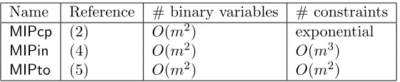
In Table 1, we compare the MIP models introduced in this section. Although all three MIP models haveO(m2) binary variables,MIPtohas more binary variables thanMIPcpand
MIPin due to Okq’s. MIP models MIPin and MIPto have polynomially many constraints,
whereas MIPcp has exponentially many constraints. MIPto has the smallest number of constraints among the three MIP models. In the computational experiment, we use a variation of the cutting plane algorithm forMIPcpas it has exponentially many constraints. ForMIPin andMIPto, we do not use a cutting plane algorithm.
3. Algorithms based on Topological Order
Name Reference # binary variables # constraints
MIPcp (2) O(m2) exponential
MIPin (4) O(m2) O(m3)
MIPto (5) O(m2) O(m2)
Table 1: Number of binary variables and constraints of MIP models
O(m2) binary variables and O(m2) constraints. In order to deal with larger graphs, we propose iterative algorithms for (1) based on Property 1. Observe that, if we are given a topological order of the nodes, thenZ and O are automatically determined in (5). In other words, we can easily obtain a subset of the arcs such that all of the arcs can be used without creating a cycle. Let ¯R be the determined adjacency matrix given topological order ¯π. In detail, we set
¯
Rjk = 1 if ¯πj >π¯k, ¯Rjk = 0 otherwise.
Letadj(¯π) be the function generating ¯R given input topological order ¯π. If we are given ¯π, then we can generate ¯R by adj(¯π), and solving (1) can be written as
min
Y F(Y) s.t.
¯
R≥supp(Y). (6)
Note that (6) has acyclic constraint ¯R ≥ supp(Y), not ¯R = supp(Y). The inequality is needed when we try to obtain a sparse solution, i.e., only a subset of the arcs is selected among all possible arcs implied by ¯R. As long as we satisfy the inequality, Y forms an acyclic subgraph. Hence, ¯R can be different from adjacency matrix supp(Y) in an optimal solution of (6), and any arc (j, k) such that ¯Rjk = 1 can be selected without creating a
cycle. For this reason, we call ¯R an adjacency candidate matrix. The algorithms proposed later in this section solve (6) by providing different ¯π and ¯R = adj(¯π) in each iteration. In fact, (6) is separable into m sub problems if F is separable. Let Yk and Zk be the kth
columns ofY and R, respectively, for nodek. Then, solving
min
Yk
Fk(Yk) s.t. R¯k≥supp(Yk), (7)
for allk∈J gives the same solution as solving (6) ifF is separable asF(Y) =P
k∈JFk(Yk).
In Section 3.1, a local improvement algorithm for a given topological order is presented. The algorithm swaps pairs of nodes in the order. In both of the iterative algorithms proposed in Sections 3.2 and 3.3, we use the local improvement algorithm presented in the following section.
3.1 Topological Order Swapping Algorithm
Algorithm 1 tries to improve the solution by swapping the topological order. In each iteration, the algorithm determines the nodes to swap that have order s1 and s2 in Line 3, where s2 =s1+ 1 implies that we select two nodes which are neighbors in the current topological order. Then in Line 4, the actual node indicesk1 and k2 such thatπk1 =s1 and πk2 =s2 are detected. The condition in Line 5 is to avoid meaningless computation when Y∗ is sparse. If |Yk∗
2k1|> 0, we know for sure that Y
∗
k1 andk2 and thus we will get a different solution. However, if Yk∗2k1 = 0, we will still have Yk∗2k1 = 0 after the swap forced by the new order. In Line 6, we create a new topological order ¯π by swapping nodesk1 and k2 inπ∗. After obtaining adjacency candidate matrix ¯R in Line 7, we solve (6) with ¯R. It is worth noting that, if F is separable, we only need to solve (7) with k= k1 and k2 because the values of ¯R are the same with R∗ except fork1 and k2 as the order difference was 1 in π∗. In Line 9, we update the best solution if the new solution is better. The iterations continue until there is no improvement in the past
m iterations, which implies that we would swap the same nodes if we proceed after this iteration. Algorithm 1 is illustrated by the following toy example.
Algorithm 1 TOSA (Topological Order Swapping Algorithm) Require: Y0,R0,π0
Ensure: Best solution Y∗, R∗, π∗
1: (Y∗, R∗, π∗)← (Y0, R0, π0), t←0
2: Whilethere is an improvement in the pastm iterations 3: t←t+ 1, s1 ←(t mod (m−1)) + 1,s2 ←s1+ 1 4: (k1, k2)← node indices satisfyingπk1 =s1 and πk2 =s2
5: If |Yk∗
2k1|>0 then
6: ¯π← π∗, ¯πk1 =s2, ¯πk2 =s1
7: R¯ ←adj(¯π)
8: Y¯ ← solve (6) with ¯R
9: If F( ¯Y)< F(Y∗)then update (Y∗, R∗, π∗) 10: End if
11: End While
Example 1 Consider a graph with m = 4 nodes. Let us assume that inputs are π0 = (2,3,1,4)with corresponding order 3−1−2−4,
Y0 =
0 0 0.5 0 0 0 0.5 0
0 0 0 0
0.4 0.8 0.1 0
, and R0=
0 0 1 0 0 0 1 0 0 0 0 0 1 1 1 0
.
In iteration 1, t= 1, s1 = 1, s2 = 2, k1 = 3, and k2 = 1. Hence, we are swapping nodes 3
and 1. Since|Y13∗|= 0.5>0,π¯ = (1,3,2,4)is created in Line 6, where the associated order
is1−3−2−4. If π¯ gives an improved objective function value, then π∗ is updated in Line
9. Let us assume that π∗ is not updated. In iteration 2, t= 2, s1 = 2, s2= 3, k1= 1, and
k2= 2. Since |Y21∗|= 0, Lines 6 - 9 are not executed.
3.2 Iterative Reorering Algorithm
used as a topological order. The selected arcs by the topological order give updates on arc weights. Let us first define notation.
ν = uniform random variable on [νlb, νub], νlb<1< νub
ρjk = pre-determined merit score of arc (j, k) for j∈J, k∈J
wjk = weight of arc (j, k) for j∈J, k∈J
ck = score of node k,k∈J
The range [νlb, νub] of the uniform random variable ν balances the randomness and
struc-tured scores. Note thatρjk should be determined based on the data and the characteristic
of the problem considered, where larger ρjk implies that arc (j, k) is attractive. Based on
the arc merit scores ρ, the score for node k,k∈J, is defined as
ck=ν·
X
j∈Jk
wjkρjk
, k∈J, (8)
which can be interpreted as a weighted summation of ρjk’s multiplied by perturbation
random number ν. Hence, nodes with high scores are attractive. Initially, all arcs have equal weights and the weights are updated in each iteration based on the topological order in the iteration. If ¯R=adj(¯π) is the adjacency candidate matrix in the iteration, then, the weights are updated by
wjk =wjk+ 1, if ¯Rjk = 1. (9)
The overall algorithmic framework is summarized in Algorithm 2. In Line 1, weights
wjk’s are initialized to 1 and ¯t, which counts the number of iterations without a best
solution update, is initialized. Also, a random order π∗ of the nodes is generated, and the corresponding solution becomes the best solution. In each iteration, first node scores ck’s
are calculated (Line 3), then topological order ¯πis obtained by sorting the nodes, and finally adjacency candidate matrix ¯R is generated (Line 4). Then, in Lines 5 and 6, solution ¯Y is obtained by solving (6) with ¯R and the best solution is updated if available. In Lines 7 -10,TOSAis executed if the current solution is within a certain percentageαfrom the best solution. Lines 11 and 12 update ¯t, and Line 13 updateswjk’s. This ends the iteration and
the algorithm continues until ¯π is converged or there is no update of the best solution in the lastt∗ iterations. Algorithm 2 is illustrated by the following toy example.
Example 2 Consider a graph with m = 3 nodes. In the current iteration, let us assume that we are given
ρ=
0 0.5 0.5 0.2 0 0.2 0.3 0.3 0
and w=
0 1 2 1 0 1 2 1 0
.
Note that we haveP
j∈J1wj1ρj1= 0.2·1 + 0.3·2 = 0.8,Pj∈J2wj2ρj2= 0.5·1 + 0.3·1 = 0.8,
and P
j∈J3wj3ρj3 = 0.4·2 + 0.2·1 = 1. If random numbers (ν) are 0.9, 1.1, 0.8 for nodes
1,2, and 3, respectively, then by (8), c1 = 0.9 ·0.8 = 0.72, c2 = 1.1·0.8 = 0.88, and
c3 = 0.8 ·1 = 0.8. Then in Line 4, we obtain π¯ = (3,1,2), with corresponding order 2−3−1, and R¯ = [0,1,1; 0,0,0; 0,1,0]. After obtaining Y¯ and updating the best solution
Algorithm 2 IR (Iterative Reordering)
Require: Merit score ρ∈Rm×m, termination parametert∗,TOSAexecution parameterα
Ensure: Best solution Y∗, R∗, π∗
1: wjk ←1,π∗ ← a random order,R∗ ←adj(π∗), ¯π←π∗,Y∗ ←solve (6) withR∗, ¯t←0
2: While(i) ¯π is not convergent or (ii) ¯t < t∗
3: Calculate score ck by (8)
4: π¯ ←sort nodes with respect to ck, ¯R←adj(¯π)
5: Y¯ ← solve (6) with ¯R
6: If F( ¯Y)< F(Y∗) thenupdate (Y∗, R∗, π∗) 7: If F( ¯Y)< F(Y∗)·(1 +α)
8: (Y0, R0, π0)←TOSA( ¯Y ,R,¯ π¯),
9: If F(Y0)< F(Y∗) thenupdate (Y∗, R∗, π∗) 10: End If
11: If (Y∗, R∗, π∗) is updatedthen ¯t←0 12: Elset¯←¯t+ 1
13: Update weights by (9) 14: End While
wnew=
0 1 2 1 0 1 2 1 0
+ ¯R =
0 2 3 1 0 1 2 2 0
This ends the current iteration.
3.3 Gradient Descent Algorithm
In this section, we propose a gradient descent algorithm based on Property 1. The algo-rithm iteratively executes: (i) moving toward an improving direction by gradients, (ii) DAG structure is recovered and topological order is obtained by a projection step. The algorithm is based on the standard gradient descent framework while the projection step takes care of the acyclicity constraints by generating a topological order from the current (possibly cyclic) solution matrix. In order to distinguish the solutions with and without the acyclicity property, we use the following notation.
Ut∈Rm×m = decision variable matrix without acyclicity requirement in iterationt
Yt∈Rm×m = decision variable matrix satisfyingG(supp(Yt))∈ Ain iteration t
Letγt be the step size in iterationt,∇F(Yt) be the derivative ofF atYt, andGt∈Rm×m
be a weight matrix that weighs each element. We assumek∇F(Yt)k∞≤M1 for a constant
M1, wherek · k∞ is the uniform (infinity) norm. The update formula
updatesYt based on the weighted gradient, where◦represents the entrywise or Hadamard product of the two matrices. Given topological orderπt, we defineGt as
Gtjk =1 + 1
πtk πkt
, j∈Jk (11)
to balance gradients of the nodes with different orders (small and large values of πkt). For nodesk1 and k2 withπtk1 = 1 andπ
t
k2 =m, most of the gradients for nodek1 are zero and
most of the gradients for node k2 are nonzero. Weight (11) tries to adjust this gap. Note that we have 2≤Gtjk ≤efor any largem. Since Ut may not satisfy acyclic constraints, in order to obtain a DAG, the algorithm needs to solve the projection problem
Y∗ = argminY kY −Utk22 s.t. G(supp(Y))∈ A, (12) wherek · k2 is the L2 norm.
Proposition 2 If Ut is arbitrary, then optimization problem (12) is N P-hard.
Proof Recall that feedback arc set is N P-complete (Karp, 1972) and maximum acyclic subgraph is the dual of the feedback arc set problem. With Ut = 1, (12) becomes the weighted maximum acyclic subgraph problem. Therefore, (12) is N P-complete.
Because solving (12) to optimality does not guarantee an optimal solution for (1), we use a greedy strategy to solve (12). The greedy algorithm, presented in Algorithm 3, sequentially determines and fixes the topological order of a node where in each iteration the problem is solved optimally given the currently fixed nodes and corresponding orders. The detailed derivations of the algorithm and the proof that each iteration is optimal, given already fixed node orders, are available in Appendix 6. In other words, we show that Line 3 is ‘locally’ optimal, i.e., it selects the best next node given that the orderq+ 1, q+ 2,· · ·, m
is fixed. In each iteration, in Line 3, the algorithm first calculates score P
j∈J¯( ¯Ujkt )2 for each node k in ¯J and picks node k∗ with the minimum value. Then, in Line 4, the order of the selected node is fixed to q. The fixed node is then excluded from the active set ¯J
and iterateq is decreased by 1 in Line 5. At the end of the algorithm, we can determine ¯Y
based on the order ¯π determined and (18) in Appendix 6. We illustrate Algorithm 3 by the following example.
Example 3 Consider a graph with m = 3 nodes. Given Ut, the algorithm returns Y¯
presented in the following.
Ut=
0 1 2 4 0 2 5 2 0
Y¯ =
0 0 0 4 0 2 5 0 0
Algorithm 3 starts with q = 3 and J¯= {1,2,3}. In iteration 1, node 2 is selected to have
π2 = 3 based on argmin{42+ 52,12+ 22,22 + 22}. Then, set J¯and integer q are updated
to J¯ = {1,3} and q = 2. In iteration 2, node 3 is selected to have π3 = 2 based on
argmin{52,22}. Then, set J¯and integer q are updated to J¯={1} and q = 1. In iteration
3, node 1 is selected. Hence, we have node order 1-3-2 and we obtain Y¯ presented above
with objective function value kY¯ −Utk2
Algorithm 3 Greedy Require: Ut∈Rm×m
Ensure: Y¯ feasible to (12), topological order ¯π
1: q←m, ¯J ←J
2: WhileJ¯6=∅ 3: k∗ = argmink∈J¯
n X
j∈J¯
(Ujkt )2o 4: π¯k∗ =q
5: J¯←J¯\ {k∗}, q←q−1 6: End While
7: Determine ¯Y by (18) in Appendix 6
The overall gradient descent algorithm for (1) is presented in Algorithm 4. In Line 1, the algorithm generates a random orderπ∗ and obtain correspondingR∗andY∗and save them as the best solution. In each iteration of the loop, Lines 3-6 follow the standard gradient descent algorithm. The weighted gradient Ht is calculated in Line 3, and the step size is determined in Line 4 based on the ratio between maxj∈Jk,k∈J|Hjkt |and maxj∈Jk,k∈J|Yjkt|.
In Line 5, the solution is updated based on the weighted gradient and, in Line 6, the greedy algorithm is used to obtain the projected solution and the topological order. Observe that we do not directly use the projected solution. This is because the projected solution is not necessarily optimal givenπt+1. Hence, in Line 7, a new solutionYt+1 is obtained based on
πt+1. In Lines 9 - 12,T OSAis executed if the current solution is within a certain percentage from the current best solution. Lines 13 and 14 update ¯tand Line 15 copies Y∗ toYt+1 if ¯
t≥t∗2 in order to focus on the solution space nearY∗. The algorithm continues untilYt is convergent or ¯t≥t∗1.
In gradient based algorithms, it is common to have γtdepend only on t, but in our case
dependency onHtandYtis justifiable since we multiply the gradient by Gt. We next show the convergence of Yt in Algorithm 4 when t∗1 = t∗2 = ∞. This makes the algorithm not to terminate unless Yt has converged and modification of Yt in Line 15 is not executed. Further, we assume the following for the analysis.
Assumption 1 For any non-zero elementYjkt,j, k∈J, ofYtin any iterationt, we assume
ε <|Yjkt|< M2, where ε is a small positive number and M2 is a large enough number. Note that Assumption 1 is a mild assumption, as ignoring near-zero values of Yt happens in practice anyway due to finite precision. For notational convenience, letLt=γt∇F(Yt)◦
Gt=γtHtbe the second term in (10). Then,Utcan be written asUt=Yt−Lt=Yt−γtHt. In the following lemma, we show that the node orders converge.
Lemma 3 If t is sufficiently large satisfying √t > (M1e)2 ε(√M2
2+ε2/m−M2)
, then πt=πt+1.
Algorithm 4 GD (Gradient Descent)
Require: Parameterst∗1 and t∗2,TOSAexecution parameterα
Ensure: Best solution Y∗, R∗, π∗
1: t←1, ¯t←0,π∗← a random order,R∗ ←adj(π∗),Y∗ ← solve (6) with R∗
2: While(i) Yt is not convergent or (ii) ¯t < t∗1
3: Ht← ∇F(Yt)◦Gt,Gt defined in (11) 4: γt← kH
tk
∞
kYtk∞
√ t
5: Ut←Yt−γtHt
6: πt+1← Greedy(Ut)
7: Yt+1← solve (6) with Rt+1 =adj(πt+1)
8: If F(Yt+1)< F(Y∗) then(Y∗, R∗, π∗)←(Yt+1, Rt+1, πt+1) 9: If F( ¯Y)< F(Y∗)·(1 +α)
10: (Y0, R0, π0)←T OSA(Yt+1, Rt+1, πt),
11: If F(Y0) < F(Y∗) then (Y∗, R∗, π∗) ← (Y0, R0, π0),(Yt+1, Rt+1, πt+1) ← (Y0, R0, π0)
12: End If
13: If (Y∗, R∗, π∗) is updatedthen ¯t←0 14: Elset¯←¯t+ 1
15: If t¯≥t∗2 then Yt+1←Y∗ 16: t←t+ 1
17: End While
show that there is no change in the node order when the condition √t > (M1e)2 ε(√M2
2+ε2/m−M2)
is met, where M1 and M2 are the upper bounds for k∇F(Yt)k∞ and kYtk∞, respectively, as assumed. We first derive
kLtk∞=
γ
tHt ∞=
1 √
t
kHtk∞ kYtk∞H
t ∞≤
1 √
t
kHtk∞
2 kYtk∞ <
1 √
t
(M1e)2
ε , (13)
where the last inequality holds since (i) kYtk∞ > ε by Assumption 1, (ii) kHtk∞ = k∇F(Yt)◦Gtk∞ ≤ M1e because k∇F(Yt)k∞ ≤ M1 by the assumption and kGtk∞ ≤ e, whereeis natural number.
Now let us consider q = ¯q in Algorithm 3 to decide node order ¯q in iteration t+ 1 and assume πktr = πkt+1r for r = m, m−1,· · ·,q¯−1. Note that we currently have ¯J = {k1, k2,· · · , kq¯}.
1. For kq¯, we derive Pj∈J¯(Ujkt q¯)2 =Pj∈J¯(Yjktq¯−Ltjkq¯)2 = Pj∈J¯(Ltjkq¯)2 < m(M1e)
2
√
tε
2 ,
where the second equality holds sinceYt
jkq¯ = 0 for allj ∈
¯
J since πkq¯= ¯q and no arc
can be used to the nodes in ¯J, and the last inequality holds due to (13) and |J¯| ≤m.
P
j∈J¯(Ujktr)2 = Pj∈J¯(Yjktr −Ltjkr)2
= P
j∈J¯(Yjktr)2+Pj∈J¯(Ljkt r)2−2Pj∈J¯Yjktr ·Ltjkr
> P
j∈J¯(Yjktr)2−2Pj∈J¯Yjktr ·Ltjkr
> ε2−2P
j∈J¯Yjktr ·Ltjkr ≥ ε2−2P
j∈J¯|Yjktm·L
t jkr|
> ε2−2M2m(M1e)
2
√
tε
where the fourth line holds due to |Yjkt
r| > ε by Assumption 1, and the sixth line
holds due to |Yjkt| ≤M2,|J¯| ≤m, and |Ltjkr|<
(M√1e)2
tε by (13).
Combining the two results forkq¯andkr∈J¯\ {kq¯}, we obtainPj∈J¯(Ujktq¯)2< m(M1e)
2
√
tε
2 <
ε2−2M2m(M1e)
2
√
tε <
P
j∈J¯(Ujktr)2, for anyr∈ {1,2,· · · ,q¯−1}, where the second inequality holds due to the condition √t > (M1e)2
ε( √
M2
2+ε2/m−M2)
. The result implies that we must have
πkt+1 ¯
q =π
t
kq¯ = ¯q by Line 3 in Algorithm 3.
Note that, when ¯q = m, we have J = ¯J and the assumption of πtkr = πtk+1r for
r = m, m−1,· · · ,q¯−1 automatically holds. By iteratively applying the above deriva-tion technique fromq=mto 1, we can show that πt=πt+1.
When (6) is solved with the identical node orders, the resulting solutions are equivalent. Hence, the following proposition holds.
Proposition 4 In Algorithm 4, Yt converges in t.
4. Estimation of Gaussian Bayesian Networks
In this section, we introduce the Gaussian Bayesian network learning problem, which follows the form of (1). The goal is to learn or estimate unknown structure between the nodes of a graph, where the error is normally distributed. The network can be estimated by optimizing a score function, testing conditional independence, or a mix of the two, as described in Section 1. Among the three categories, we select the score based approach with the L1 -penalized least square function recently studied in Han et al. (2016).
Let X ∈Rn×m be a data set with n observations and m features. Let I = {1,· · · , n}
and J = {1,· · ·, m} be the index set of observations and features, respectively. For each
k∈J, we build a regression model in order to explain featurek using a subset of variables inJk. In other words, we set featurek as the response variable and a sparse subset of Jk
as explanatory variables of the regression model for variablek. In order to obtain a subset of Jk, the LASSO penalty function is added. Considering regression models for all k ∈J
Let βjk,j∈Jk,k∈J, be the coefficient of attributej for dependent variable k. Then
the problem can be written as
min
β
1
n X
k∈J
X
i∈I
(xik−
X
j∈Jk
βjkxij)2+λ
X
k∈J
X
j∈Jk
|βjk| s.t. G(supp(β))∈ A, (14)
which follows the form of (1). In Han et al. (2016), individual weights are used for the penalty term, i.e., λP
k∈J
P
j∈Jkwjk|βjk|, however, in the computational experiment, we
set all weights equal to 1 for simplicity.
LetZjk = 1 if attributejis used for dependent variablekandZjk = 0 otherwise. Then,
we can formulate MIPto for (14) as
min 1
n X
k∈J
X
i∈I
(xik−
X
j∈Jk
βjkxij)2+λ
X
k∈J
X
j∈Jk
|βjk| (15a)
s.t. |βjk| ≤M Zjk, j∈Jk, k∈J, (15b)
Zjk−mZkj ≤
X
r∈J
r(Okr−Ojr), j∈Jk, k∈J, (15c)
Zjk+Zkj ≤1, j∈Jk, k∈J, (15d)
X
q∈J
Okq= 1, k∈J, (15e)
X
k∈J
Okq= 1, q∈J, (15f)
Z, O∈ {0,1}m×m, (15g)
βjk not restricted, j∈Jk∪ {0}, k∈J, (15h)
where M is a large constant. Note that (15b) is the linear constraint corresponding to
Z =supp(Y) in (5). Similarly, (15a), (15b), (4c) - (4e) and (15h) can be used to formulate
MIPin for (14). ForMIPcp, (15a), (15b), (15h), and the constraints in (2) can be used for (14).
Note thatMin (15b) plays an important role in computational efficiency and optimality. IfMis too small, the MIP model cannot guarantee optimality. IfM is too large, the solution time can be as large as enumeration. The algorithm for getting a valid value forM in Park and Klabjan (2013) can be used. However, the valid value of big M for multiple linear regression is often too large (Park and Klabjan, 2013). For (15), we observed that a simple heuristic presented in Section 5 works well.
In each iteration of IR (Algorithm 2) and GD (Algorithm 4), we are given topological order ¯π and matrix ¯R = adj(¯π). Let Sk = {j ∈ Jk|R¯jk = 1} be the set of selected
candidate arcs for dependent variable k. Given fixed ¯R, (14) is separable into m LASSO linear regression problems
min 1
n X
i∈I
(xik−
X
j∈Sk
βjkxij)2+λ
X
j∈Sk
5. Computational Experiment
For all computational experiments, a server with two Xeon 2.70GHz CPUs and 24GB RAM is used. Although there are many papers studying Bayesian network learning with various error measures and penalties, here we focus on minimizing the LASSO type objective (SSE and penalty) and we picked one of the latest paper of Han et al. (2016) with the same objective function as a benchmark.
The MIP models MIPcp,MIPin, andMIPto are implemented with CPLEX 12.6 in C#. For MIPcp, instead of implementing the original cutting plane algorithm, we use CPLEX Lazy Callback, which is similar to the cutting plane algorithm. Instead of solving (3) to optimally from scratch in each iteration, we solve (2) with Lazy Callback, which allows updating (adding) constraints (cycle prevention constraints) in the process of the branch and bound algorithm whenever an integer solution with cycles is found. Given a solution with the cycles, we detect all cycles and add cycle prevention constraints for the detected cycles.
For MIPcp,MIPin, and MIPto, we set big M as follows. Givenλ, we solve (14) without acyclic constraints. Hence, we are allowed to use all arcs inJkfor each modelk∈J. Then, we obtain the estimated upper bound for bigM by
M = 2 max
j∈Jk,k∈J|βjk|
. (17)
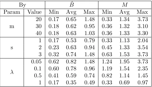
We observed that the above formula gives large enough bigM for all cases in the following experiment. In Appendix 6, we present comparison of regression coefficients of implanted network (DAG) with big M values by (17). The result shows that the big M value in (17) is always valid for all cases considered.
We compare our algorithms and models with the algorithm in Han et al. (2016), which we denote as DIST here. Their algorithm starts with neighborhood selection (NS), which filters unattractive arcs and removes them from consideration. The procedure is specifi-cally developed for high dimensional variable selection when m is much larger than n. In our experiment, many instances considered are not high dimensional and some have dense solutions. Further, by filtering arcs, there exists a probability that an arc in the optimal solution can be removed. Hence, we deactivated the neighborhood selection step of their original algorithm, where the R script of the original algorithm is available on the journal website.
For GD and IR, the algorithms are written in R (R Core Team, 2016). We use glmnet
package (Friedman et al., 2010) functionglmnet for solving LASSO linear regression prob-lems in (16). For IR, we use parameters α = 0.01, t∗ = 10, νlb = 0.8, and νub = 1.2. For GD, we use parameters α= 0.01,t∗1 = 10, and t∗2 = 5. Because both GD and IR start with a random solution, they perform different with different random solutions. Further, since we observe that the execution time of GDandIR are much faster thanDIST, we decided to runGDand IR with 10 different random seeds and report the best solution. To emphasize the number of different random seeds forGDand IR, we use the notationGD10andIR10in the rest of the section.
We first test all algorithms with synthetic instances generated using R package pcalg
(Kalisch et al., 2012). FunctionrandomDAGis used to generate a DAG and functionrmvDAG
a DAG is generated by randomDAG function. Next, the generated DAG and random co-efficients are used to create each column (with standard normal error added) by rmvDAG
function which uses linear regression as the underlying model. After obtaining the data matrix from the package, we standardize each column to have zero mean with standard de-viation equal to one. The DAG used to generate the multivariate data is considered as the true structure or true arc set while it may not be the optimal solution for the score function. The random instances are generated for various parameters described in the following.
m: number of features (nodes)
n: number of observations
s: expected number of true arcs per node
d: expected density of the adjacency matrix of the true arcs
By changing the ranges of the above parameters, three classes of random instances are generated.
Sparse data sets: The expected total number of true arcs is controlled by s and most of the instances have a sparse true arc set. We use n ∈ {100,200,300}, m ∈ {20,30,40,50}, and s ∈ {1,2,3} to generate 10 instances for each (n, m, s) triplet. This yields a total of 360 random instances.
Dense data sets: The expected total number of true arcs is controlled by dand most of the instances have a dense true arc set compared with the sparse data sets. We use n ∈ {100,200,300}, m ∈ {20,30,40,50}, and d ∈ {0.1,0.2,0.3} to generate 10 instances for each (n, m, d) triplet, and thus we have a total of 360 random instances.
High dimensional data sets: The instances are high dimensional (m ≥ n) and very sparse. The expected total number of true arcs is controlled by s. We use n = 100 and m∈ {100,150,200}, ands∈ {0.5,1,1.5}to generate 10 instances for each (m, s) pair, which yields a total of 90 random instances.
We use four λvalues differently defined for each data set in order to cover the expected number of arcs with the four λ values. For each sparse instance, we solve (14) with λ ∈ {1,0.5,0.1,0.05}. For dense data sets, a wide range ofλvalues are needed to obtain selected arc sets that have similar cardinalities with the true arc sets. Hence, for each dense instance, instead of fixed values over all instances in the set, we useλvalues based on expected density
d: λ=λ0·10−(10·d−1), whereλ0 ∈ {1,0.1,0.01,0.001}. For each high dimensional instance, we use λ∈ {1,0.8,0.6,0.4}. Observe that the expected densities of the adjacency matrices vary across the three data sets. The sparse instances have expected densities between 0.02 and 0.15, the dense instances have expected densities between 0.1 and 0.3, and the high dimensional instances have expected densities between 0.002 and 0.015. Hence, different ranges of λvalues are necessary.
For all of the results presented in this section, we present the average performance by
n, m, s, d and λ. For example, the result for n = 100 and m = 20 are the averages of 120 and 90 instances, respectively. In all of the comparisons, we use the following metrics.
time: computation time in seconds
δsol: relative gap (%) from the best objective value among the compared algorithms
the relative gap from the best of the three objective function values obtained by the MIP models.
kzk0: number of arcs selected (number of nonzero regression coefficients βjk’s)
In comparing the performance metrics, we use plot matrices. In each Figure 1, 2, 3, 5, and 6, multiple bar plots form a matrix. The rows of the plot matrix correspond to performance metrics and the columns stand for parameters used for result aggregation. For example, the left top plot in Figure 1 shows execution times of the algorithms where the results are aggregated by n (the number of observations), because the first row and first column of the plot matrix in Figure 1 are for execution times andn, respectively.
In Section 5.1, we compare the performance of iterative algorithms GD10and IR10 and the benchmark algorithmDIST. In Section 5.2, we compare the performance of MIP models
MIPcp,MIPin, and MIPto. We also compare all models and algorithms with a subset of the synthetic instances in Section 5.2. Finally, in Section 5.4, we solve a popular real instance of Sachs et al. (2005) in the literature.
5.1 Comparison of Iterative Algorithms
In this section, we compare the performance of GD10, IR10, and DIST by time, δsol, and
kzk0 for each of the three data sets.
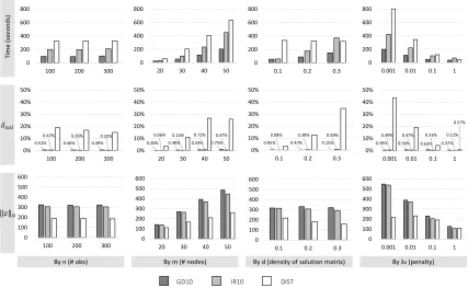
In Figure 1, the result for the sparse data sets is presented. The bar plot matrix presents the performance measures aggregated by n, m, s, and λ.
By m (# nodes) By s (# arcs per node) By λ (penalty)
Time
(se
con
d
s)
GD10 IR10 DIST
By n (# obs) 0
50 100 150
100 200 300
0 50 100 150
20 30 40 50
0 50 100 150
0.05 0.1 0.5 1
0 50 100 150
1 2 3
0.0% 0.2% 0.4% 0.6% 0.8% 1.0% 1.2%
100 200 300
0.0% 0.2% 0.4% 0.6% 0.8% 1.0% 1.2%
20 30 40 50
0.0% 0.2% 0.4% 0.6% 0.8% 1.0% 1.2%
0.05 0.1 0.5 1
0.0% 0.2% 0.4% 0.6% 0.8% 1.0% 1.2%
1 2 3
0 100 200 300 400
100 200 300
0 100 200 300 400
20 30 40 50
0 100 200 300 400
0.05 0.1 0.5 1
0 100 200 300 400
1 2 3
𝛿𝑠𝑜𝑙
𝑧 0
The computation time of all three algorithms increases in increasingmand decreasingλ, where the computation time of DISTincreases faster than the other two. The computation time of DISTis approximately 10 times faster than theGD10time whenλ= 1, but 2 times slower when λ = 0.05. With increasing n, the computation times of all algorithms stay the same or decrease. This can be seen counter-intuitive because larger instances do not increase time. However, a larger number of observations can make predictions more accurate and could reduce search time for unattractive subsets. Especially, the computation time of DIST decreases in increasing n. We think this is because more observations give better local selection in the algorithm when adding and removing arcs. The number of selected arcs (kzk0) of GD10 and IR10 is greater than DIST for all cases because the topological order based algorithms are capable of using the maximum number of arcs
m(m−1) 2
, while arc selection based algorithms, such as DIST, are struggling to select many arcs without violating acyclic constraints. In terms of the solution quality, all algorithms have δsol less
than 1.2% and perform good. However, we observe several trends. Asλdecreases (required to select more arcs), GD10 and IR10 start to outperform. We also observe that, as the problem requires to select more arcs (increasingm, increasings, and decreasingλ), GD10
and IR10 perform better. As n increases, δsol of GD10 and DIST decrease, whereas δsol of IR10 increases.
The result for the dense data sets is presented in Figure 2. The bar plot matrix presents the performance measures aggregated by n, m, d, and λ0. Recall that, for the dense data set, we solve (14) with λ= λ0·10−(10·d−1) and λ0 ∈ {1,0.1,0.01,0.001}. For simplicity of presenting the aggregated result, we use λ0 in the plot matrix, while λvalues are used for actual computation.
The computation time of all three algorithms again increases in increasing m and de-creasing λ, where the computation time of DISTincreases faster than the other two. Com-pare to the result for the sparse data sets, the execution times are all larger for the dense data set. The number of selected arcs (kzk0) of GD10and IR10 is again greater thanDIST
for all cases, where kzk0 is twice larger for GD10 and IR10 when m or d is large, or λ is small. In terms of the solution quality, GD10 and IR10 outperform in most of the cases, while δsol values of DIST increase fast in changing m, d, and λ. The values of δsol for all
algorithms are larger than the sparse data sets result. GD10 and IR10 are better for most of the cases. In general, we again observe that GD10 and IR10 perform better when the problem requires to select more arcs.
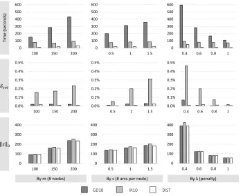
The result for the high dimensional data sets is presented in Figure 3. The bar plot matrix presents the performance measures aggregated by m, s,and λ, while n is excluded from the matrix as we fixed nto 100.
The computation time of all three algorithms again increases in increasing m and de-creasing λ. However, unlike the previous two sets, the computation times of GD10 and
IR10 increase faster than DIST. This is due to the efficiency of the topological order based algorithms. When a very small portion of the arcs should be selected in the solution, topo-logical orders are not informative. For example, consider a graph with three nodesA, B, C
By m (# nodes) By d (density of solution matrix) By λ0(penalty) Ti me (sec onds )
GD10 IR10 DIST
By n (# obs) 0
200 400 600 800
100 200 300
0 200 400 600 800
20 30 40 50
0 200 400 600 800
0.001 0.01 0.1 1 0
200 400 600 800
0.1 0.2 0.3
0.51% 0.46% 0.49% 0.47% 0.26% 0.32%
0% 10% 20% 30% 40% 50%
100 200 300
0.20% 0.40% 0.59% 0.75% 0.06% 0.15% 0.72% 0.47%
0% 10% 20% 30% 40% 50%
20 30 40 50
0.39% 0.56% 0.63% 0.37% 0.49% 0.47% 0.33% 0.12%
0.57% 0% 10% 20% 30% 40% 50%
0.001 0.01 0.1 1 0.85% 0.47% 0.15%
0.08% 0.38% 0.59%
0% 10% 20% 30% 40% 50%
0.1 0.2 0.3
0 100 200 300 400 500 600
100 200 300 0
100 200 300 400 500 600
20 30 40 50
0 100 200 300 400 500 600
0.001 0.01 0.1 1 0 100 200 300 400 500 600
0.1 0.2 0.3
𝛿𝑠𝑜𝑙
𝑧 0
Figure 2: Performance of GD10,IR10, and DIST(dense data)
by DISTdoes not have difficulties preventing cycles and the algorithm can decide whether to include arcs easier. The comparison of δsol values also show that arc based search is
competitive. Although all algorithms haveδsol values less than 0.5%, we find clear evidence
that the performance of IR10 decreases in increasingm and s and decreasingλ. Although theδsol values of GD10 andDISTare similar, considering the fast computing time of DIST,
we recommend to use DISTfor very sparse high dimensional data.
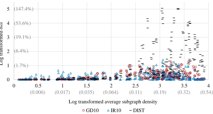
In Figure 4, we present combined results of all three data sets by relating solution densities and δsol. Observe that, for each quadruplet of n, m, s(or d), λ, we have results
from 10 random instances for each algorithm. Valueδsol is the average of the 10 results for
each quadruplet and for each algorithm, AvgDen is the average density of the adjacency matrices of the 10 results and the three algorithms. In Figure 4, we present a scatter plot of
ln(1+AvgDen) andln(1+100·δsol). Each point in the plot is the average of 10 results by an
algorithm and each algorithm has 324 points displayed 1. The numbers in the parenthesis along the axes are the corresponding values ofδsolandAvgDen. In the plot, we first observe
that the algorithms perform similarly when the solutions are sparse and theδsol values have
large variance when the solutions are dense. When the log transformed solution density is less than 2, the averageδsol values of GD10,IR10, andDISTare 0.06%, 0.15%, and 0.04%,
respectively. However, the solution quality of DIST drastically decreases as the solutions become denser. This makes sense because sparse solutions can be efficiently searched by
By m (# nodes) By s (# arcs per node) By λ(penalty) 𝛿𝑠𝑜𝑙 Ti me (sec onds) 0 100 200 300 400 500 600
100 150 200
0 100 200 300 400 500 600
0.4 0.6 0.8 1
0 100 200 300 400 500 600
0.5 1 1.5
0.0% 0.1% 0.2% 0.3% 0.4% 0.5%
100 150 200
0.0% 0.1% 0.2% 0.3% 0.4% 0.5%
0.4 0.6 0.8 1
0.0% 0.1% 0.2% 0.3% 0.4% 0.5%
0.5 1 1.5
0 100 200 300 400
100 150 200
0 100 200 300 400
0.4 0.6 0.8 1
0 100 200 300 400
0.5 1 1.5
𝑧 0
GD10 IR10 DIST
Figure 3: Performance of GD10,IR10, and DIST(high dimensional data)
arc-based search, while dense solutions are not easy to obtain by adding or removing arcs one by one. This also explains the relatively small and largeδsolvalues for dense and spares
solutions, respectively, by the topological order based algorithms. BetweenGD10andIR10, we do not observe a big difference.
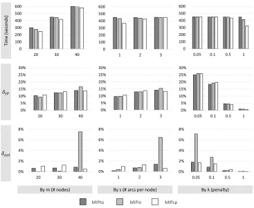
5.2 Comparison of MIP Models
In this section, we compare the performance of MIPto,MIPin, andMIPcp using time,δsol,
and kzk0 and the following additional metric.
δIP: the optimality gap (%) obtained by CPLEX within allowed 15·m seconds
Due to scalability issues of all models, we only use the sparse data with m= 20,30,40. We also limitn= 100. For all instances, we use the 15·m seconds time limit for CPLEX. For example, we have a time limit of 300 seconds for instances withm= 20.
The result is presented in Figure 5. Comparing the time of all models with the time limit for CPLEX, we observe thatMIPinandMIPcpwere able to terminate with optimality for several instances when m = 20 and λ = 1. This implies that MIPin and MIPcp are efficient when the problem is small and the number of selected arcskzk0 is small. However, in general, δIP values tend to be consistent with different models, while they increase in
0 1 2 3 4 5
0 0.5 1 1.5 2 2.5 3 3.5 4
Lo
g
t
ra
n
sfo
rm
ed
δ
sol
Log transformed average subgraph density
GD10 IR10 DIST
(1.7%) (6.4%) (19.1%) (53.6%) (147.4%)
(0.54) (0.32)
(0.19) (0.11)
(0.064) (0.035)
(0.017) (0.006)
Figure 4: Scatter plot of δsol and average solution densities
found for δIP for all models. By comparing δsol values, we observe that MIPinis best when m= 20 and 30. However, the performance of MIPin drops drastically as m and sincrease andλdecreases. Actually,MIPinfails to obtain a reasonably good solution within the time limit for several instances. This gives large δsol values and increases the average. The δsol
values of MIPto are smaller thanMIPcpwhen mand sare small, whileMIPcpoutperforms when m= 40 ors= 3.
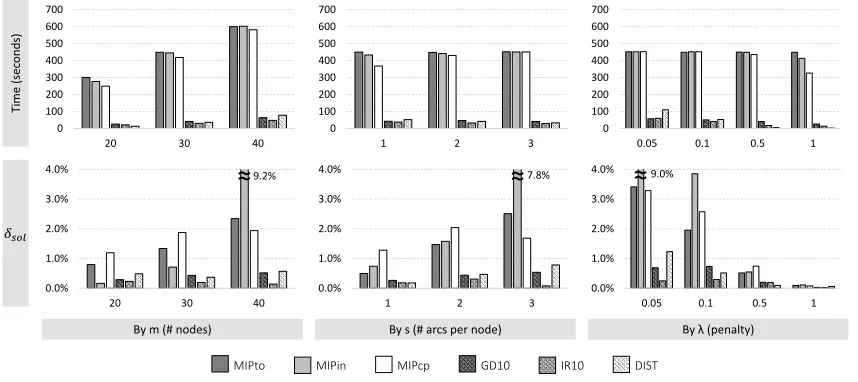
5.3 Comparison of all MIP Models and Algorithms
In Figure 6, we compare all models and algorithms for selected sparse instances withn= 100 and m ∈ {20,30,40}, which were used to test MIP models. In the plot matrix, we show the average computation time and δsol (gap from the best objective value among the six
models and algorithms) bym, s,and λ. Note that δsol values of a few MIPinresults are not
fully displayed in the bar plots due to their large values. Instead, the actual numbers are displayed next to the corresponding bar. The result shows that MIP models spent more time while the solution qualities are inferior in general. The values ofδsolfor the MIP models
are competitive only whenλis large, which requires sparse solution. However, even for this case, MIP models spend longer time than the algorithms. Hence, ignoring the benefit of knowing and guaranteeing optimality by the MIP models, we conclude that the algorithms perform better for all cases.
By m (# nodes) By s (# arcs per node) By λ (penalty)
MIPto MIPin MIPcp
0% 5% 10% 15% 20% 25% 30%
20 30 40
0% 5% 10% 15% 20% 25% 30%
0.05 0.1 0.5 1 0% 5% 10% 15% 20% 25% 30%
1 2 3
0% 2% 4% 6% 8%
20 30 40
0% 2% 4% 6% 8%
1 2 3
0% 2% 4% 6% 8%
0.05 0.1 0.5 1
𝛿𝑠𝑜𝑙 𝛿𝐼𝑃 0 100 200 300 400 500 600
20 30 40
0 100 200 300 400 500 600
1 2 3
0 100 200 300 400 500 600
0.05 0.1 0.5 1
Ti
me (sec
onds)
Figure 5: Performance of MIPto, MIPin, and MIPcp (sparse data with n = 100 and m ∈ {20,30,40})
5.4 Real Data Example
In this section, we study the flow cytometry data set from Sachs et al. (2005) by solving (14). The data set has been studied in many works including Friedman et al. (2008), Shojaie and Michailidis (2010), Fu and Zhou (2013), and Aragam and Zhou (2015). The data set is often used as a benchmark as the casual relationships (underlying DAG) are known. It has n = 7466 cells obtained from multiple experiments with m = 11 measurements. The known structure contains 20 arcs. For the experiment, we standardize each column to have zero mean with standard deviation equal to one.
In Table 2, we compare the performance of the three algorithms GD10,IR10, andDIST
for various values ofλ. The MIP models are excluded due to scalability issue2. We compare the previously used performance measures execution time, solution cardinalities (kzk0), and solution quality (δsol). In addition, we also compare sensitivities (true positive ratio) of the
solutions. By comparing with the known structure with 20 arcs, we calculate directed true
By m (# nodes) By s (# arcs per node) By λ(penalty)
Ti
me
(sec
onds
)
GD10 IR10 DIST
0.0% 1.0% 2.0% 3.0% 4.0%
20 30 40
0.0% 1.0% 2.0% 3.0% 4.0%
1 2 3
0.0% 1.0% 2.0% 3.0% 4.0%
0.05 0.1 0.5 1
0 100 200 300 400 500 600 700
20 30 40
0 100 200 300 400 500 600 700
1 2 3
0 100 200 300 400 500 600 700
0.05 0.1 0.5 1
MIPto MIPin MIPcp
9.2% 7.8% 9.0%
≈
≈
≈
𝛿𝑠𝑜𝑙
Figure 6: Performance of all models and algorithms (sparse data with n = 100 and m ∈ {20,30,40})
positive (dTP) and undirected true positive (uTP). If arc (j, k) is in the known structure, dTP counts only if arc (j, k) is in the algorithm’s solution, whereas uTP counts either of arcs (j, k) or (k, j) is in the algorithm’s solution.
The solution times of the three algorithms are all within a few seconds, as m is small. Also, the solution cardinalities (kzk0) are similar. The best δsol value among the three
algorithms in each row is in boldface. We observe that GD10 provides the best solution (smallest δsol) in most cases and IR10 is the second best. The δsol values of DISTincrease
as λ increases. This is consistent with the findings in Section 5.1. Note that the density of the underlying structure is 20/112 = 0.165, which is dense. This explains the good performance of GD10 and IR10. On the other hand, even though GD10 provides the best objective function values for most of the cases, the dTP and uTP values of GD10 are not always the best. The highest value among the three algorithms in each row is in boldface. Whileδsol values of DISTare the largest among the three algorithms, dTP and uTP values
are the best in some cases. When λ is small, DIST tends to have higher dTP and uTP. However, asλincreases,GD10 gives the best dTP and uTP values. To further improve the prediction power, we may need weighting features or observations.
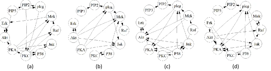
From Table 2, we observe that a slight change in solution quality δsol affects the final
selection of DAG significantly. Also, the best objective function value does not necessarily give the highest true positive value since the L1-norm penalized least square (14) may not be the best score function. In Figure 7, we present the graphs of known casual interactions (a), estimated subgraph byGD10(b),IR10 (c), andDIST(d). All graphs are obtained with
λ= 0.25, but the numbers of arcs are different (see Table 2). In fact, the difference between
GD10 IR10 DIST
λ time kzk0 δsol dTP uTP time kzk0 δsol dTP uTP time kzk0 δsol dTP uTP
0.5 14.6 9 0.00% 0.22 0.56 10.8 9 0.22% 0.22 0.56 5.8 9 0.38% 0.56 0.56
0.45 13.7 11 0.00% 0.27 0.55 10.9 13 0.30% 0.15 0.46 8.5 9 0.49% 0.56 0.56
0.4 14.3 11 0.00% 0.27 0.55 14.8 13 0.36% 0.15 0.46 7.0 13 0.61% 0.38 0.46 0.35 16.0 13 0.00% 0.23 0.54 12.4 17 0.42% 0.12 0.41 8.6 15 0.73% 0.33 0.47 0.3 15.1 13 0.00% 0.23 0.46 14.3 17 0.21% 0.24 0.41 8.0 17 0.84% 0.29 0.47
0.25 14.4 16 0.00% 0.38 0.56 14.8 20 0.22% 0.25 0.50 6.7 20 0.94% 0.30 0.50 0.2 16.0 16 0.00% 0.31 0.56 14.6 22 0.31% 0.32 0.55 6.8 21 1.12% 0.33 0.52 0.15 16.4 21 0.00% 0.33 0.57 15.6 25 0.32% 0.32 0.52 9.5 23 1.26% 0.30 0.52 0.1 17.4 24 0.00% 0.25 0.50 11.0 28 0.26% 0.07 0.43 9.1 27 1.45% 0.26 0.44 0.05 17.7 28 0.32% 0.39 0.50 11.5 30 0.00% 0.10 0.47 10.1 32 1.87% 0.22 0.41
Table 2: Performance on the real data set from Sachs et al. (2005)
(a) (b) (c) (d)
Figure 7: Known DAG (a) and estimated subgraphs with λ= 0.25 by GD10(b), IR10 (c), andDIST(d)
6. Conclusion
We propose an MIP model and iterative algorithms based on topological order. Although the computational experiment is conducted for Gaussian Bayesian network learning, all the proposed model and algorithms are applicable for problems following the form in (1). While many MIP models and algorithms are designed based on arc search, using topological order provides some advantages that improve solution quality and algorithm efficiency.
1. DAG constraints (acyclicity constraints) are automatically satisfied when arcs from high order nodes to low order nodes are used.
2. In applying the concept for MIP, a lower number of constraints is needed (O(m2)) whereas arc based modeling can have exponentially many constraints in the worst case.
3. In applying the concept in designing iterative algorithms, one of the biggest merits is the capability of utilizing the maximum number of arcs possible (m(m2−1)), while arc based algorithms struggle with using all possible arcs.
benefit when the solution matrix is dense. The result presented in Section 5.1 clearly indicates that the topological order based algorithms outperform when the density of the resulting solution is high. On the other hand, arc-based search algorithms, represented by DIST in our experiment, can be efficient when the desired solutions are very sparse.
Appendix A. Greedy Algorithm for Projection Problem
In this section, we present the detail derivations and proofs of Algorithm 3 (greedy). The algorithm sequentially determines topological order by optimizing the projection problem given an already fixed order up to the iteration point. Solving the projection problem is N P-complete and our algorithm may not give a global optimal solution. However, the result of this section shows that Algorithm 3 gives an optimal choice of the next node to have fixed order given pre-fixed orders.
We start by describing some properties of Y∗ in the following three lemmas. For the following lemmas, letπ∗j represent the topological order of nodej defined byY∗.
Lemma 5 For any Yjk∗, we must have either Yjk∗ = 0 or Yjk∗ =Ujkt .
Proof For a contradiction, let us assume that there exist indicesq andrsuch that Yqr∗ 6= 0 and Yqr∗ 6= Uqrt . Let us create a new solution ¯Y such that ¯Y = Y∗ except ¯Yqr = Uqrt .
Note that ¯Y is a feasible solution to (12) becausesupp( ¯Y) ≤supp(Y∗) element-wise since
Yqr∗ 6= 0. Further, we havekY∗−Utk2 >kY¯−Utk2 because (Yqr∗ −Uqrt )2>0 = ( ¯Yqr−Uqrt )2
and ¯Y =Y∗ except Yqr∗ 6= ¯Yqr. This contradicts optimality ofY∗.
Note that Lemma 5 implies that solving (12) is essentially choosing between 0 andUjk∗ for
Yjk∗. This selection is also based on the following property.
Lemma 6 If π∗j > π∗k, then Yjk∗ =Ujkt .
Proof For a contradiction, let us assume that there exist indicesqandrsuch thatYqr∗ 6=Ut qr
while πq∗> π∗r. Let us create a new solution ¯Y such that ¯Y =Y∗ except ¯Yqr=Uqrt .
1. IfYqr∗ 6= 0, then ¯Y is a DAG sincesupp( ¯Y)≤supp(Y∗) element-wise.
2. IfYqr∗ = 0, then arc (q, r) can be used in the solution without creating a cycle because
πq∗> πr∗. Hence, ¯Y is a DAG.
Therefore, ¯Y is a feasible solution to (12). However, it is easy to see that kY¯ −Utk2 <
kY∗−U∗k2 because (Yqr∗ −Uqrt )2 >0 = ( ¯Yqr−Uqrt )2. This contradicts optimality ofY∗.
Given the topological order byY∗, let ˆJk={j ∈Jk|π∗
j > πk∗}be the subset ofJk such that
the nodes in ˆJk are earlier than nodek. Combining Lemmas 5 and 6, we conclude that Y∗
has the following structure.
Yjk∗ = (
Ujkt ifj∈Jˆk,
0 ifj∈J\Jˆk, k∈J (18)
Further, we can calculate node k’s contribution to the objective function value without explicitly using Y∗.
Lemma 7 For each node k∈J, it contributes
X
j∈J\Jˆk
(Ujkt )2
to the objective function value for (12). In other words, the contribution of node k is the
Proof For node k, we can derive
P
j∈J(Y
∗
jk−Ujkt )2 =
P
j∈J\Jˆk(Yjk∗ −Ujkt )2 =
P
j∈J\Jˆk(Ujkt )2,
where both equal signs are due to (18). The first equality is due to Yjk∗ =Ujkt for j ∈ Jˆk
and the second equality holds sinceYjk∗ = 0 for j∈J\Jˆk.
We next detail the derivation of the greedy algorithm presented in Algorithm 3. Let ¯
J ⊆J be the index set of yet-to-be-ordered nodes and ¯Jc= J\J¯be the index set of the nodes that have already been ordered. The procedure is equivalent to iteratively solving
k∗ = argmink∈J¯ n
min
Yk
X
j∈J
(Yjk −Ujkt )2
o
, (19)
whereYk= [Y1k, Y2k,· · ·, Ymk]∈Rm×1 is the column in Y corresponding to node k. Set ¯J
is updated by ¯J = ¯J\ {k∗} and πk∗∗ =|J¯|after solving (19). We propose an algorithm to
solve (19) based on the properties of Y∗ described in Lemmas 5 - 7. Given ¯J, we solve
k∗ = argmink∈J¯ n X
j∈J¯
(Ujkt )2 o
. (20)
Next, we show that solving (20) gives an optimal solution ¯Yjk∗, j ∈ Jk to (19). We can
actually replicate the properties of Y∗ for ¯Yjk∗.
Lemma 8 An optimal solution to (19) must have either Y¯jk∗ = 0 or Y¯jk∗ =Ut
jk∗ for all j∈Jk.
Lemma 9 An optimal solution to (19) must haveY¯jk∗=Ut
jk∗ for j∈J\J¯.
Lemma 10 An optimal solution to (19) must satisfy P
j∈J( ¯Yjk∗−Ut jk∗)2 =
P
j∈J¯(Ujkt ∗)2
The proofs are omitted as they are similar to the proofs of Lemmas 5 - 7, respectively. Note that, by Lemma 10, we show the equivalence ofP
j∈J(Yjk∗−Ut
jk∗)2 andPj∈J¯(Ujkt ∗)2. This
result also holds for each term, k∈J¯, of the argmin function in (19). Hence, the following lemma holds.
Lemma 11 Solving (20) is equivalent to solving (19).
Observe that (20) is used in Line 3 of the greedy algorithm in Algorithm 3. Hence, by property (19), the algorithm gives an optimal choice of node to be fixed with the pre-fixed topological order.
Appendix B. Summary Statistics for Maximum Coefficients