The Thirty-Third AAAI Conference on Artificial Intelligence (AAAI-19)
Multi-Agent Path Finding for Large Agents
∗Jiaoyang Li
CS Department Univ. of Southern CaliforniaPavel Surynek
Faculty of Information TechnologyCzech Technical University [email protected]
Ariel Felner
SISE Department Ben-Gurion UniversityHang Ma
T. K. Satish Kumar
Sven Koenig
CS Department Univ. of Southern CaliforniaAbstract
Multi-Agent Path Finding (MAPF) has been widely studied in the AI community. For example, Conflict-Based Search (CBS) is a state-of-the-art MAPF algorithm based on a two-level tree-search. However, previous MAPF algorithms as-sume that an agent occupies only a single location at any given time, e.g., a single cell in a grid. This limits their ap-plicability in many real-world domains that have geometric agents in lieu of point agents. Geometric agents are referred to as “large” agents because they can occupy multiple points at the same time. In this paper, we formalize and study LA-MAPF, i.e., MAPF for large agents. We first show how CBS can be adapted to solve LA-MAPF. We then present a gen-eralized version of CBS, called Multi-Constraint CBS (MC-CBS), that adds multiple constraints (instead of one con-straint) for an agent when it generates a high-level search node. We introduce three different approaches to choose such constraints as well as an approach to compute admis-sible heuristics for the high-level search. Experimental re-sults show that all MC-CBS variants outperform CBS by up to three orders of magnitude in terms of runtime. The best variant also outperforms EPEA* (a state-of-the-art A*-based MAPF solver) in all cases and MDD-SAT (a state-of-the-art reduction-based MAPF solver) in some cases.
1
Introduction
In robotics and computer games, one has to find collision-free paths for multiple agents operating in a common envi-ronment. This has led to the study of Multi-Agent Path Find-ing (MAPF) in the AI community, where we are required to find a path for each agent from its given start vertex to its given goal vertex on a given graph such that no two agents collide with each other at any given time. MAPF can be ap-plied to warehouse robots (Wurman, D’Andrea, and Mountz
∗
The research at the University of Southern California was sup-ported by the National Science Foundation (NSF) under grant num-bers 1409987, 1724392, 1817189 and 1837779 as well as a gift from Amazon. The research was also supported by the United States-Israel Binational Science Foundation (BSF) under grant number 2017692 and the Czech Science Foundation (GACR) under grant number 19-17966S. The views and conclusions contained in this document are those of the authors and should not be interpreted as representing the official policies, either expressed or implied, of the sponsoring organizations, agencies or the U.S. government. Copyright c2019, Association for the Advancement of Artificial Intelligence (www.aaai.org). All rights reserved.
2008), office robots (Veloso et al. 2015), aircraft-towing ve-hicles (Morris et al. 2016), video game characters (Ma et al. 2017) and many other domains.
Numerous optimal MAPF algorithms have been devel-oped in recent years, including reduction-based algorithms (Yu and LaValle 2013a; Erdem et al. 2013; Surynek et al. 2016), A*-based algorithms (Standley 2010; Wagner and Choset 2011; Goldenberg et al. 2014) and dedicated search-based algorithms (Sharon et al. 2013; 2015; Bo-yarski et al. 2015; Felner et al. 2018). See (Ma et al. 2016a; Felner et al. 2017) for complete surveys.
Although previous MAPF algorithms have found some real-world applications (H¨onig et al. 2016), they are based on one simplistic assumption that limits their applicability. This assumption is to ignore the shape of agents and con-sider them as point agents, which occupy exactly one point at any time. In reality, agents are geometric in nature with definite shapes. Therefore, they typically occupy a set of points at any time. We refer to such agents aslarge agents. MAPF algorithms can be applied to large agents by lower-ing the resolution of discretization of the environment. How-ever, this degrades their performance and thus their practical applicability.
To address these concerns, we formally studyMulti-Agent Path Finding for Large Agents(LA-MAPF) which takes into consideration the shapes of agents. This consideration also addresses the case where agents have to maintain a safety distance from each other since a virtual boundary can now be defined for each agent. Intuitively, LA-MAPF is harder to solve than MAPF since it is a generalization of MAPF and agents are more likely to collide with each other.
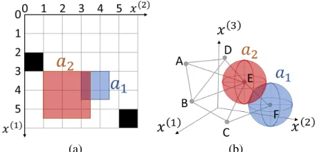
vari-(a) (b)
Figure 1: Shows two examples of two agents colliding with each other. (a) shows a 4-neighbor 2D grid with square-shaped agents, where lines represent edges, intersection points represent vertices, and black cells represent obstacles. (b) shows a 3D roadmap with sphere-shaped agents.
ants of MC-CBS, adapted EPEA* and adapted MDD-SAT.1 EPEA* (Goldenberg et al. 2014) is a state-of-the-art A*-based MAPF solver, and MDD-SAT (Surynek et al. 2016) is a start-of-the-art reduction-based MAPF solver. All MC-CBS variants outperform MC-CBS by up to three orders of mag-nitude in terms of runtime. The best variant also outperforms EPEA* in all cases and MDD-SAT in some cases.
2
Problem Definition and Related Concepts
We formalize LA-MAPF as follows: We are given an undi-rected graphG= (V, E)embedded in ad-dimensional Eu-clidean space (usuallyd = 2,3). Each vertex v ∈ V is a point in the Euclidean space that is specified by its coordi-nates(v(1), . . . , v(d)). We are also given a set ofk agents{a1. . . ak} with unique start and goal vertices, and each agent has a fixed geometric shape around a reference point that cannot undergo transformations like rotations. We say that an agent is at a vertexv when its reference point is at vertexv, and we say that an agent traverses an edge(u, v)
when its reference point moves along edge(u, v). Ifaiis at vertexv, then the set of points occupied byaiis denoted by Si(v). Figure 1(a) shows an example of two square-shaped agents on a 2D grid. Their reference points are the top-left corners.a1 (blue) is at vertexv = (3,3) with an 1.5×1.5
square shape S1(v) = {(x(1), x(2)) | 0 ≤ x(j)−v(j) ≤ 1.5, j = 1,2}, and a2 (red) is at vertex u = (3,1) with
a 2.5×2.5 square shape S2(u) = {(x(1), x(2)) | 0 ≤ x(j)−u(j) ≤ 2.5, j = 1,2}. Figure 1(b) shows another
example on a 3D roadmap where two sphere-shaped agents
a1(blue) anda2 (red) are at vertices F and E, respectively.
Their reference points are the sphere centers.
On the same graph G, different agents have different traversable subgraphs because of their different shapes (e.g., in Figure 1(a), a1 can be at (0,0) while a2 cannot). This
subgraphGi = (Vi, Ei)is called the configuration space of ai. We assume that the start and goal vertices of each agent are in the same connected component of its
configu-1
We refer to the adapted versions of CBS, EPEA* and MDD-SAT also as CBS, EPEA* and MDD-MDD-SAT, respectively.
ration space. At each discrete timestept,ai can eitherwait at its current vertexv ∈ Vi, ormove to an adjacent vertex u, where(v, u)∈Ei. Both wait and move actions have unit costs unlessaiterminally waits at its goal vertex.
In MAPF, a conflict between two agents is either a ver-tex conflict, where two agents are at the same verver-tex at the same timestep, or an edge conflict, where two agents traverse the same edge in opposite directions at the same timestep. In LA-MAPF, however, agents could collide when they are in close proximity with each other. Therefore, we general-ize the definitions of conflicts. We define avertex conflict
as a five-element tuplehai, aj, u, v, ti, where the shapes of ai andaj overlap ifai is at vertexuandaj is at vertexv at the same timestept. Similarly, we define anedge conflict
as a seven-element tuplehai, aj, u1, u2, v1, v2, ti, where the
shapes ofaiandajoverlap ifaimoves from vertexu1tou2
andaj moves from vertexv1 tov2 at the same timestept.
We assume that there exists a conflict detection function that checks entire paths and returns all vertex conflicts and edge conflicts. Our task is to find a set of conflict-free paths that move all agents from their start vertices to their goal vertices with minimum sum of costs of all paths.
Previous research has also used generalized conflicts. H¨onig et al. (2018) considered the shape of large agents like quadrotors and defined three new types of generalized conflicts: vertex-vertex conflicts, vertex-edge conflicts and edge-edge conflicts, where the first one is a special case of our vertex conflicts and the two other ones are special cases of our edge conflicts. They solved the problem by adapting ECBS (Barer et al. 2014), a suboptimal version of CBS, to their problem in a way similar to the adapted CBS that we introduce in Section 3.2. We show in Section 3.2 that this kind of direct adaptation is inefficient in many cases. Using a different perspective, Atzmon et al. (2018) generalized the definition of a conflict from a timestep to a time range in order to obtain robust plans.
3
Conflict-Based Search (CBS)
LA-MAPF is NP-hard, since it generalizes MAPF, which is NP-hard (Yu and LaValle 2013b; Ma et al. 2016b). In this section, we review Conflict-Based Search for MAPF and in-troduce its direct adaption to LA-MAPF.
3.1
CBS for MAPF
Conflict-Based Search(CBS) (Sharon et al. 2015) is a two-level search-based algorithm that is complete and optimal for MAPF. Its high level performs a best-first search on a binaryconstraint tree(CT). Each CT node contains a set of constraints, where a constraint is either avertex constraint
hai, u, ti that prohibits agentai from being at vertexuat timesteptor anedge constrainthai, u1, u2, tithat prohibits ai from moving fromu1 tou2 at timestep t, and a set of
paths for all agents that satisfy all constraints. Thecostof the CT node is the sum of costs of all paths. The CT root node contains an empty set of constraints and a set of individual shortest paths.
paths. If they are conflict-free, thenN is a goal node and CBS returns its paths. Otherwise, the high level arbitrarily chooses and resolves a vertex conflicthai, aj, u, v, ti(u=v in MAPF) or an edge conflicthai, aj, u1, u2, v1, v2, ti(u1= v2 andu2 = v1 in MAPF) by splitting N into two child
CT nodes,N1andN2, that inherit all constraints and paths
from N. The high level also adds a new vertex constraint hai, u, tior edge constrainthai, u1, u2, titoN1and a new
vertex constrainthaj, v, tior edge constrainthaj, v1, v2, ti
toN2and then runs a low-level search for both child nodes
to find shortest paths for all agents that satisfy the new set of constraints in each of them. Since each child node has one additional constraint imposed on only one agent, the low-level search needs to re-plan the path for only that one agent.
Improved CBS (ICBS) (Boyarski et al. 2015) improves CBS by classifying conflicts and choosing to resolve car-dinal conflicts first. A conflict is cardinal if, when CBS uses this conflict to split a CT node, the cost of each one of the two resulting child nodes is larger than the cost of the CT node. CBSH (Felner et al. 2018) improves it further by aggregating cardinal conflicts and computing admissible heuristics to guide the high-level search.
3.2
CBS for LA-MAPF
Similar to techniques used in (H¨onig et al. 2018), CBS can be directly adapted to LA-MAPF by considering generalized conflicts and changing the conflict detection function to the one discussed in Section 2. However, the resulting version of CBS is very inefficient for large agents. For example, in Figure 1(a), a1 tries to move from(3,0) to(3,4), anda2
tries to move from(0,1)to(3,1). In the CT root node, both agents follow their individual shortest paths and have vertex conflicts at timesteps1,2and3. The drawing is a snapshot that shows their vertex conflict at timestep 3. If CBS chooses to resolve this vertex conflict, then the right child node has a new constraintha2,(3,1),3i.a2is forced to wait for one
timestep and thus stays at vertex(2,1)at timestep3. How-ever,a2then still conflicts witha1at timestep3in this child
node. The conflict betweena1anda2at timestep3is
there-fore not resolved by this split. Although it will be resolved eventually, many intermediate CT nodes are generated.
4
Multi-Constraint CBS (MC-CBS)
The above observations motivate the idea of adding multi-ple constraints in a single CT node expansion. We present a new algorithm, MC-CBS, which adds multiple constraints for the same timestep to child nodes in order to resolve mul-tiple related conflicts in a single CT node expansion, which resembles lookahead reasoning at the high level and can re-sult in smaller CTs, thus making the search more efficient.We say that two vertex or edge constraints foraiandaj respectively aremutually disjunctiveiff any pair of conflict-free paths for ai and aj satisfies at least one of the two constraints, i.e., there do not exist two conflict-free paths such that both constraints are violated. In particular, the con-straints that CBS adds to two child nodes are always mutu-ally disjunctive. We say that two sets of constraints are mu-tually disjunctiveiff each constraint in one set is mutually
disjunctive with each constraint in the other set. Intuitively, working with mutually disjunctive constraint sets gives us the power of constraint propagation.
When MC-CBS resolves a conflict hai, aj, u, v, ti (or
hai, aj, u1, u2, v1, v2, ti) in a CT nodeN, it generates two
child nodes with N’s current constraint set and additional constraint sets,C1andC2, respectively:
1. C1andC2include thecore constraintsthat CBS uses to
resolve the conflict, i.e.,hai, u, ti ∈ C1 andhaj, v, ti ∈ C2(orhai, u1, u2, ti ∈C1andhaj, v1, v2, ti ∈C2).
2. C1 andC2 are enhanced with other constraints that
en-sure thatC1andC2remain mutually disjunctive.
Different strategies for choosingC1andC2are discussed
in Sections 4.1 and 4.2. Here, we show that MC-CBS is com-plete and optimal.
Lemma 1(Optimality). If MC-CBS terminates, it returns a set of conflict-free paths with the minimum sum of costs.
Proof. The proof has two parts. We first show that, for a given CT nodeN with constraint setC, any set of conflict-free paths that satisfyCalso satisfy at least one of the con-straint setsCSC
1andCSC2. This is true because,
oth-erwise, there would exist two conflict-free paths such that both of them are consistent withCbut one path violates a constraintc1 ∈ C1 and the other one violates a constraint c2∈C2. Then,c1andc2are not mutually disjunctive,
con-tradicting the assumption. Therefore, the expansion of a CT node does not lose any set of conflict-free paths.
The second part is the same as the proof of optimality for CBS (Sharon et al. 2015). The cost of a CT node is a lower bound on the sum of costs of conflict-free paths that satisfy its constraint set. The high-level search chooses to expand a CT node with minimum cost and the expansion does not lose any conflict-free paths. So the cost of the chosen CT node is always a lower bound on the sum of costs of all conflict-free paths. Therefore, the set of paths of the first CT node chosen for expansion whose paths are conflict-free is indeed a set of conflict-free paths with the minimum sum of costs.
Lemma 2(Completeness). MC-CBS terminates if there ex-ists a set of conflict-free paths.
Proof. The costs of CT nodes are non-decreasing in expan-sion order because MC-CBS runs a best-first search and the costs of child nodes are at least as large as the costs of their parents. In addition, there are a finite number of CT nodes for a given costc, because there are only a finite number of possible conflicts withinctimesteps and, once a conflict is resolved at CT nodeN, it does not reappear in the subtree ofN. Therefore, a set of conflict-free paths must be found after expanding a finite number of CT nodes.
There are numerous ways to generalize the core con-straints to two mutually disjunctive constraint sets for MC-CBS. For example, in Figure 1(a), the two sets first in-clude the core constraints, i.e.,C1 = {ha1,(3,3),3i}and C2={ha2,(3,1),3i}. We can add constraints for other
ver-tices toC1andC2, such asha2,(2,1),3itoC2(becausea1
add constraints for other timesteps, such as ha2,(3,2),4i
toC2 (because, no matter where a1 moves from (3,3) at
timestep3, it conflicts witha2being at(3,2)at timestep4).
In this paper, we only add constraints for the same timestep to keep MC-CBS simple. In general, it is hard to determine whether two constraints for different timesteps are mutually disjunctive. Moreover, we can often find equiv-alent (e.g., block the same set of paths) or better (e.g., block a larger set of paths) constraint sets to add for the same timestep. In Figure 1(a), the pair of constraint sets {ha1,(3,3),3i} and {ha2,(3,1),3i,ha2,(3,2),4i} is no
better than the pair of constraint sets{ha1,(3,3),3i} and
{ha2,(x, y),3i | 2 ≤ x≤ 4,1 ≤y ≤ 3} becausea2can
only be at vertex(x, y),2≤x≤4,1≤y≤3, at timestep
3to reach vertex(3,2)at timestep4.
In Sections 4.1 and 4.2, we introduce three approaches for choosing constraint sets for MC-CBS. In Section 4.3, we present a new representation of constraint sets to speed up MC-CBS for regular shaped agents. We only discuss the constraint sets for vertex conflicts since the constraint sets for edge conflicts can be derived analogously.
4.1
Asymmetric and Symmetric Approaches
Consider the resolution of a vertex conflicthai, aj, u, v, ti. Two mutually disjunctive constraint sets can be built asym-metrically or symasym-metrically.21. Theasymmetric approach(ASYM) adds a constraint set of size one{hai, u, ti}to the left child node that prohibits agentai from being at its current vertexvat timestept and a large constraint set{haj, v0, ti | hai, aj, u, v0, tiis a vertex conflict} to the right child node that prohibits agentaj from being at any vertex at timesteptwhere it could collide withai.
2. Thesymmetric approach(SYM) chooses a pointpin the Euclidean space that is inside the overlap areaSi(u)∩ Sj(v), and then adds one constraint set to each child node. The constraint set blocks all vertices that the agent could be at while including p in its shape, i.e., C1 =
{hai, v0, ti |p∈Si(v0), v0 ∈V}andC2={haj, v0, ti | p ∈ Sj(v0), v0 ∈ V}. Unlike ASYM, that adds a straint set of size one to one child node and a large con-straint set to the other child node, SYM adds concon-straint sets of similar cardinalities to both child nodes.
For example, in Figure 1(a), ASYM adds{ha1,(3,3),3i}
to one child node and{ha2,(x, y),3i | 1 ≤ x, y ≤ 4}to
the other child node. But SYM adds{ha1,(x, y),3i | 2 ≤ x, y ≤ 3} to one child node and {ha2,(x, y),3i | 1 ≤ x, y ≤ 3} to the other child node when the chosen point
pis (3.25,3.25). Thus, ASYM adds 17 constraints in to-tal while SYM adds only 13 constraints in toto-tal. However, we empirically show in Section 6.1 that SYM usually out-performs ASYM, perhaps because SYM usually has more pairs of mutually disjunctive constraints, e.g., 36 pairs in this
2
Atzmon et al. (2018) introduced similar asymmetric and sym-metric approaches to add multiple constraints, although they stud-ied a different problem and added constraints for the same vertex at different timesteps.
example. Since each such pair may block some conflicting paths, SYM usually results in smaller search spaces.
Another important observation is that not all constraints generated by SYM or ASYM are relevant. Some con-straints are irrelevant because they block vertices that are not reachable by the agents at the given timestep, such as ha2,(4,1),3igiven that the start vertex ofai is(0,1), and some constraints are less relevant because they block the ver-tices that can be reached only when paths are very long, such asha2,(1,4),3igiven that the start vertex and the goal
ver-tex ofa2 are (0,1) and(3,1), respectively. Therefore, we
present a more intelligent approach that aims to add more relevant constraints in the next section.
4.2
Maximizing the Costs of Child Nodes
When splitting a CT node, large costs of both child nodes mean more progress for the high-level search. Thus, the costs of the child nodes can be used to measure the relevance of a constraint set. ICBS (Boyarski et al. 2015) utilizes this insight by choosing cardinal conflicts whenever available, where both child nodes have higher costs than their parent node. Here, we try to find a pair of constraint sets where the child nodes have the highest possible costs.
Calculating the weights of constraint sets. A Multi-Valued Decision Diagram (MDD) (Sharon et al. 2013)
M DDµi is a directed acyclic graph that consists of all paths of costµfor agentaifrom its start vertex to its goal vertex. All nodes at deptht of M DDiµ correspond to all vertices whereaican be at timestepten route such a path. There-fore, if a constraint set for timesteptblocks all vertices of
M DDµi at deptht, the cost of the agent’s new path is at leastµ+ 1after adding it. Conversely, if a constraint set for timesteptdoes not block all vertices ofM DDµi at deptht, the cost of the agent’s new path is at mostµafter adding it.
ICBS usesM DDiµto predict whether the cost ofai’s path isµor higher after adding a constraint. Here, we generalize this idea and useM DDµi+d to predict whether the cost of
ai’s path isµ, . . . , µ+dor at leastµ+d+ 1after adding a constraint set.d∈Nis called thelookahead depth, and the predicted cost increment in {0,1, . . . , d+ 1}is called the
weightof the constraint set.
Given a CT node N and an agent ai whose path is of cost µ, we build M DDµi+d. During this construction, we also assign a weight wto each MDD node(v, t)such that
µ+wequals the cost ofai’s shortest path moving from its start vertex to its goal vertex via vertexvat timestept, i.e.,
(v, t)∈M DDiµ+wand(v, t)∈/ M DDiµ+w−1. The weight of a constraint set C0 for ai at timestep t is calculated as follows. Consider all MDD nodes at deptht: (1) IfC0 does not block all MDD nodes with weight0, then the cost ofai’s path after addingC0does not change, and thus the weight of
Algorithm 1:A template for MaxWeight-d.
Input:Vertex conflicthai, aj, u, v, ti, and depthd.
Output:Constraint sets,C1andC2, and weights,w1andw2.
1 C1← {hai, u, ti};
2 C2← {haj, v0, ti | hai, aj, u, v0, tiis a vertex conflict}; 3 w1←getWeight(C1);w2←getWeight(C2);
4 forw01=w1+ 1 :d+ 1do
5 C10 ← {hai, u0, ti |(u0, t)∈M DDµi+dand its weight < w10}//µis the cost ofai’s shortest path.
6 C20 ← {haj, v0, ti | haj, v0, tiis mutually disjunctive
with every constraint inC01}; 7 ifhaj, v, ti∈/C20then 8 break;
9 w02←getWeight(C20);
10 if{w10, w02}is better than{w1, w2}then
11 C1, C2, w1, w2←C1, C0 20, w01, w02;
12 returnC1,C2,w1andw2;
Maximizing the weights of constraint sets. We can now design a new approach for choosing constraint sets for MC-CBS based on maximizing their weights. We refer to this approach as MaxWeight-d(MAX-d or MAX for short). It builds MDDs for both agents with lookahead depthdand chooses thebestpair of constraint sets, i.e, the pair that max-imizes the smaller weight of the two. It breaks ties by pre-ferring the pair with the maximum sum of weights.
Algorithm 1 shows the pseudo-code for MAX. It enumer-ates all possible weights ofC1and, for each possible weight,
computes the maximum weight ofC2such thatC2includes
the core constraint and is mutually disjunctive withC1.
Ini-tially, it regards the pair of constraint sets generated by ASYM as the best pair seen so far (Lines 1-3). It then itera-tively increases the weightw10 of the first constraint set (Line 4). In each iteration, it first choosesC0
1to be of minimum
size for the given weightw01(Line 5), i.e., C10 only blocks those MDD nodes whose weights are smaller than w10. It then buildsC20 of maximum size to be mutually disjunctive withC10 (Line 6). If the core constrainthaj, v, ti∈/ C20,
indi-cating thatC10 cannot have a weight equal to or larger than w01, it just returns the best constraint sets and weights found so far (Lines 7-8). Otherwise, it computes the weight ofC20
(Line 9) and updates the best constraint sets and weights if necessary (Lines 10-11).
Algorithm 1 is shown only for vertex conflicts for ease of explanation. When expanding a CT node in MC-CBS, we run Algorithm 1 for all vertex conflicts and edge conflicts and choose to resolve the conflict with the best constraint sets. Particularly, the smaller weight of two constraint sets for cardinal conflicts is always at least one, and the smaller weight of two constraint sets for other conflicts is always zero. Therefore, cardinal conflicts still have higher priority than other conflicts, which is consistent with the conflicts prioritization of ICBS.
4.3
Constraints for Regular Shaped Agents
Agents often have regular shapes, such as rectangles and cir-cles in a 2D space or cuboids and spheres in a 3D space. In such cases, two mutually disjunctive constraint sets have ge-ometric representations that can be leveraged for computa-tional benefits.For example, when all agents are rectangular, an agentai of size~si = (s
(1) i , s
(2)
i )whose reference point is the point with minimum coordinates hasSi(v) ={~p|~v ≤p~≤~v+ ~
si}. Here,~vis the vector representation of vertexvand the vector inequalities indicate that the inequalities hold for both dimensions. The tuplehai, aj, u, v, tiis a vertex conflict iff Si(u)∩Sj(v)6=∅or, equivalently,
−~sj≤~v−~u≤~si. (1)
Arectangle constraint of the formhai, ~umin, ~umax, tican be used to represent a constraint set that prohibits agent
ai from being in the rectangular area{v | ~umin ≤ ~v ≤ ~
umax} at timestept. We say that two rectangle constraints
hai, ~umin, ~umax, tiandhaj, ~vmin, ~vmax, tiaremutually dis-junctive iff their corresponding constraint sets are mutu-ally disjunctive or, equivalently,−~sj ≤ ~vmin −~umaxand ~
vmax−~umin≤~si.
We can replace the constraint setsC1andC2for MC-CBS
by two rectangle constraints. Instead of checking for each pair of constraints inC1andC2whether they are mutually
disjunctive we need to only check two diagonal vertices, and all approaches in Sections 4.1 and 4.2 can thus be simplified. For some other regular shaped agents, such as circle, cuboid or sphere shaped agents, we can use similar repre-sentations and thus simplify MC-CBS as well.
5
Adding Heuristics to MC-CBS
Felner et al. (2018) improve CBS by adding heuristics to the high-level search. A CT node’s g-value is its cost, and its ad-missible heuristic is the cost of the minimum vertex cover of an unweighted conflict graph. The conflict graph has ver-tices representing agents and edges representing cardinal conflicts between agents. Here, we generalize this model to a weighted conflict graph GCF = (VCF, ECF), where each vertex vi ∈ VCF represents an agent ai, each edge (vi, vj)∈ECFrepresents cardinal conflicts between agents ai andaj, and each pair of weightswij andwji for edge (vi, vj)represents that eitheraihas to increase its cost by at leastwijorajhas to increase its cost by at leastwjiin order to resolve this conflict. In MC-CBS, we use the weights ofC1andC2forwij andwji, respectively. Then, the optimal solution of the following Integer Linear Program (ILP) is an admissible heuristic:
minimize k X
i=1
ci (2)
s.t. ci≥wijxij, 1≤i, j≤k, i6=j
xij+xji≥1, 1≤i < j≤k
xij∈ {0,1}, 1≤i, j≤k, i6=j,
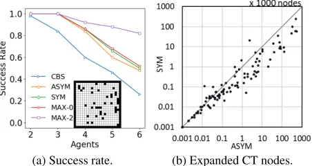
(a) Success rate. (b) Expanded CT nodes.
Figure 2: Experimental results for CBS and variants of MC-CBS on a 20×20 grid with10%blocked cells.
cover problem in (Felner et al. 2018) is a special case where allwij = 1. Similar conflict graphs and ILP models are used in the context of cost-optimal planning (Pommerening et al. 2015).
6
Experimental Results
We implemented and experimented with CBS, all MC-CBS variants (i.e., ASYM, SYM and MAX), EPEA* and MDD-SAT on grids with square agents. We also tested CBS and some MC-CBS variants on a 3D roadmap with ellipsoid agents. All CBS-based algorithms used the conflict prioriti-zation of ICBS. All algorithms were written in C++ and ran on a 2.80 GHz Intel Core i7-7700 laptop with 8 GB RAM and a runtime limit of 5 minutes. We tried both brute force search and an off-the-shelf ILP solver to solve the ILP in Equation (2) for calculating heuristics. Brute force search ran faster on small graphs while the ILP solver ran faster on large graphs. In both cases, the overhead of computing the heuristics was very small since the conflict graphs were sparse. Therefore, we simply use brute force search in our experiments.
6.1
Square Agents on a 2D Grid
We first compare the performances of CBS and all MC-CBS variants on a 4-neighbor 20×20 2D grid with10%random blocked cells. Each agent is a 2.5×2.5 square whose refer-ence point is its top-left corner. All algorithms use Equa-tion (1) to detect conflicts. All MC-CBS variants use the rectangle constraints discussed in Section 4.3. For MAX, we tested lookahead depthsdfrom 0 to 4. We used 50 instances with randomly generated start vertices and goal vertices for each number of agents.
Overall performances. Figure 2(a) shows the success rate, i.e., number of instances solved within 5 minutes, of each algorithm. The success rates of MAX with d = 1,2,3,4 are quite close to each other, so we only plotted MAX-2. Overall, CBS performs the worst since it repeatedly resolves related conflicts between the same agents. SYM, ASYM and MAX-0 perform better since they resolve a set of related conflicts in a single expansion. MAX-2 performs the best since it looks ahead several steps and takes into consid-eration the costs of child nodes. Table 1 shows the runtime
Table 1: Average runtime and number of expanded CT nodes for CBS, SYM and MAX-2 on instances solved by SYM. Cutoff time of 5 minutes is included in the average for un-solved instances.kis the number of agents.
Runtime (ms) Expanded CT nodes
k Ins. CBS SYM MAX-2 CBS SYM MAX-2
2 50 8,907 7 2 25,924 20 3
3 50 52,876 903 24 218,136 2,214 36
4 43 >98,056 22,057 2,100 >376,921 43,904 2,958 5 33 >138,875 72,703 3,056 >320,928 125,593 2,683 6 25 >199,285 116,613 6,373 >802,317 244,991 8,324
Table 2: Average runtime (ms) of MAX with different looka-head depths d. Cutoff time of 5 minutes is included in the average for unsolved instances.kis the number of agents.
k d= 0 d= 1 d= 2 d= 3 d= 4
2 6.6 1.8 1.9 1.7 2.1
3 551.1 24.0 23.6 31.6 49.3
4 43,747.1 31,612.9 29,544.7 27,391.2 28,539.8 5 104,597.3 56,336.4 51,225.3 49,273.0 55,912.9 6 152,360.1 70,675.5 61,283.5 66,329.4 68,116.7
and number of expanded CT nodes of CBS, SYM and MAX-2 on instances solved by SYM. SYM outperforms CBS by up to three orders of magnitude on both metrics, indicating that the overhead per expanded CT node is negligible for SYM. MAX-2 outperforms SYM by factors of up to 60 and 20 with respect to the number of expanded CT nodes and the runtime, respectively, indicating that it has more over-head per expanded CT node but is still beneficial overall.
Comparing ASYM and SYM. Figure 2(b) shows the number of expanded CT nodes for ASYM and SYM on in-stances solved by both algorithms. With a few exceptions, SYM outperforms ASYM not only on the success rate but also on the number of expanded CT nodes (and thus the run-time).
Comparing MAX with different lookahead depths. Ta-ble 2 compares the runtime of MAX withdranging from 0 to 4. We observe that MAX withd= 0(no lookahead) is sig-nificantly slower than the others. Asdincreases, the runtime first decreases and then increases because a larger lookahead depth has more pruning power but also incurs more over-head.d= 2or3works best in our experiments.
MAX with heuristics. Adding heuristics to MAX de-creases both the number of expanded CT nodes and the run-time, although it does not improve its success rate. For in-stance, adding heuristics to MAX-4 decreases the number of expanded CT nodes by30.1%and the runtime by21.5%
on 8-agent instances. Similar observations have been made in (Felner et al. 2018) on sparse grids, but in the next sub-section we discuss cases where adding heuristics provides a much larger speedup.
6.2
Ellipsoid Agents on a 3D Roadmap
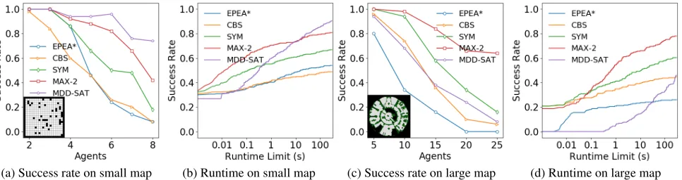
(a) Success rate on small map (b) Runtime on small map (c) Success rate on large map (d) Runtime on large map
Figure 3: Experimental results on 2D grids.
Figure 4: Shape of agents (left), reproduced from (H¨onig et al. 2018), and the structure of the roadmap (right).
Table 3: The runtime and number of expanded CT nodes on “Swap50” with a 3D roadmap.k is the number of agents. MAX+h is MAX-1 with heuristics.
Runtime (ms) Expanded CT nodes k CBS ASYM MAX-1 MAX+h CBS ASYM MAX-1 MAX+h 5 38 61 23 13 18 26 9 7
6 124 122 126 40 28 25 20 11
7 1,175 549 735 290 188 93 100 52
8 253,550 15,829 10,570 5,221 30,411 2,408 1,289 747
a 7.5 m×6.5 m×2.5 m space with ellipsoid agents. The el-lipsoids model quadrotors and their downwash effects. The ellipsoids have radii (0.15 m, 0.15 m, 0.3 m) with central reference points, as in Figure 4(left). Agents are required to fly through windows in a wall in opposite directions. The roadmap, generated by the SPARS algorithms (Dobson and Bekris 2014), has 869 vertices and 3,371 edges, as in Fig-ure 4(right). In a preprocessing step, we identify all possible vertex and edge conflicts using the swept collision model (H¨onig et al. 2018). On average, there exist 1.75 different vertex conflicts per vertex, and 24.08 different edge conflicts per edge. The original instance has 50 agents and was solved by suboptimal solvers in (H¨onig et al. 2018). We randomly chose a small subset of agents and solved the resulting in-stance with our optimal algorithms CBS, ASYM, MAX-1, and MAX-1 with heuristics.
Table 3 shows the runtime and number of expanded CT nodes. ASYM, MAX-1 and MAX-1 with heuristics decrease the runtime of CBS by factors of up to 16, 24 and 49, re-spectively. Unlike the results in Section 6.1, adding
heuris-tics here significantly reduces the number of expanded CT nodes and runtime because agents traverse narrow corridors in opposite directions, which results in more cardinal con-flicts.
6.3
Comparing with Other Solvers on 2D Grids
We now compare CBS and two MC-CBS variants, namely SYM and MAX-2, with an A*-based solver, EPEA*, and a reduction-based solver, MDD-SAT, on the same instances as in Section 6.1. We also test them on larger instances with square agents of different sizes randomly chosen from {2.5,3.5,4.5}. We used a large 4-neighbor 194×194 2D grid with51.3%blocked cells, namely the benchmark game map lak503d from (Sturtevant 2012). We used 50 instances with randomly generated start vertices and goal vertices for each number of agents.
EPEA*. A*-based MAPF solvers conduct search in the joint multi-agent state space. EPEA* (Goldenberg et al. 2014) is a lazy version which delays the generation of nodes whose costs are larger than the costs of their parents and thus avoid generating unnecessary nodes. It can be adapted to LA-MAPF by using Equation (1) to identify conflict-free actions as legal operators. This adaptation is promising since the branching factor could be smaller than the one for MAPF instances. CBS-based solvers, on the other hand, have more conflicts to resolve for LA-MAPF than for MAPF.
MDD-SAT. MDD-SAT (Surynek et al. 2016) is a SAT-based MAPF solver. It relies on the construction of a propo-sitional formula that is satisfiable iff the given MAPF in-stance has a set of conflict-free paths of a certain cost. It introduces a propositional variableXt
v(ai)for each agentai and node(v, t)inai’s MDD that is ‘true’ iff agentai is at vertexvat timestept. MDD-SAT can be modified for LA-MAPF by introducing additional variablesYt
u(ai)and con-straints involving them to reflect the shapes of agents. Here, Yt
u(ai)is ‘true’ iff there exists vertexv such thatXvt(ai)is ‘true’ and vertexu ∈ Si(v). In other words, implications
Xt
constraintsPk i=1Y
t
v(ai)≤1are used to disallow collisions between agents.
Results. Figure 3(a), Figure 3(b) present the success rates and runtimes on the small map. MAD-SAT dominates all other algorithms in terms of success rates within 5 minutes. When we vary the runtime limit, MAX-2 has the highest success rate when the runtime limit is less than10s (where instances are relatively easy), while MDD-SAT has the high-est success rate when the runtime limit is more than10 s (where instances are more difficult). Figure 3(c), Figure 3(d) present the success rates and runtimes on the large game map. MAX-2 significantly outperforms all other algorithms in all cases except when the runtime limit is less than 0.1 s.
Although it is hard to predict the performances of the al-gorithms in all domains, we can give some guidance based on these observations and analysis. MDD-SAT is strong for difficult problems in small domains. MAX is strong for easy problems or in large domains, despite the fact that its looka-head depth needs to be set appropriately.
7
Conclusions and Future Work
In this paper, we generalized MAPF to a practically viable version, called LA-MAPF, that takes into consideration the shapes of agents. We presented MC-CBS, a new algorithm that improves CBS by adding multiple constraints during the expansion of a CT node. Unlike CBS, the MC-CBS allows us to resolve multiple related conflicts in one shot, while also generalizing the use of the minimum vertex cover for heuris-tic guidance of the high-level search. We proposed three ap-proaches for choosing the constraints as well as an approach for computing the heuristics. Empirically, we showed that all MC-CBS variants outperform CBS by up to three orders of magnitude in terms of runtime, and the best variant also out-performs EPEA* in all cases and MDD-SAT in some cases. There are many directions for future work. For example, we could study the problem that allows the rotation of shapes and develop sub-optimal LA-MAPF solvers, with the expec-tation that they would be more scalable than optimal ones.References
Atzmon, D.; Stern, R.; Felner, A.; Wagner, G.; Bart´ak, R.; and Zhou, N. 2018. Robust multi-agent path finding. InSoCS, 2–9. Barer, M.; Sharon, G.; Stern, R.; and Felner, A. 2014. Suboptimal variants of the conflict-based search algorithm for the multi-agent pathfinding problem. InSoCS, 19–27.
Boyarski, E.; Felner, A.; Stern, R.; Sharon, G.; Tolpin, D.; Betza-lel, O.; and Shimony, S. E. 2015. ICBS: Improved conflict-based search algorithm for multi-agent pathfinding. InIJCAI, 740–746. Dobson, A., and Bekris, K. E. 2014. Sparse roadmap spanners for asymptotically near-optimal motion planning. The International Journal of Robotics Research33(1):18–47.
Erdem, E.; Kisa, D. G.; Oztok, U.; and Schueller, P. 2013. A general formal framework for pathfinding problems with multiple agents. InAAAI, 290–296.
Felner, A.; Stern, R.; Shimony, S. E.; Boyarski, E.; Goldenberg, M.; Sharon, G.; Sturtevant, N. R.; Wagner, G.; and Surynek, P. 2017. Search-based optimal solvers for the multi-agent pathfinding prob-lem: Summary and challenges. InSoCS, 29–37.
Felner, A.; Li, J.; Boyarski, E.; Ma, H.; Cohen, L.; Kumar, T. K. S.; and Koenig, S. 2018. Adding heuristics to conflict-based search for multi-agent path finding. InICAPS, 83–87.
Goldenberg, M.; Felner, A.; Stern, R.; Sharon, G.; Sturtevant, N. R.; Holte, R. C.; and Schaeffer, J. 2014. Enhanced Partial Expansion A*.Journal of Artificial Intelligence Research50:141– 187.
H¨onig, W.; Kumar, T. K. S.; Cohen, L.; Ma, H.; Xu, H.; Ayanian, N.; and Koenig, S. 2016. Multi-agent path finding with kinematic constraints. InICAPS, 477–485.
H¨onig, W.; Preiss, J. A.; Kumar, T. K. S.; Sukhatme, G. S.; and Ayanian, N. 2018. Trajectory planning for quadrotor swarms.IEEE Transactions on Robotics34(4):856–869.
Ma, H.; Koenig, S.; Ayanian, N.; Cohen, L.; H¨onig, W.; Kumar, T. K. S.; Uras, T.; Xu, H.; Tovey, C.; and Sharon, G. 2016a. Overview: Generalizations of multi-agent path finding to real-world scenarios. InIJCAI-16 Workshop on Multi-Agent Path Find-ing.
Ma, H.; Tovey, C.; Sharon, G.; Kumar, T. K. S.; and Koenig, S. 2016b. Multi-agent path finding with payload transfers and the package-exchange robot-routing problem. InAAAI, 3166–3173. Ma, H.; Yang, J.; Cohen, L.; Kumar, T. K. S.; and Koenig, S. 2017. Feasibility study: Moving non-homogeneous teams in congested video game environments. InAIIDE, 270–272.
Morris, R.; Pasareanu, C.; Luckow, K.; Malik, W.; Ma, H.; Kumar, S.; and Koenig, S. 2016. Planning, scheduling and monitoring for airport surface operations. InAAAI-16 Workshop on Planning for Hybrid Systems.
Pommerening, F.; R¨oger, G.; Helmert, M.; and Bonet, B. 2015. Heuristics for cost-optimal classical planning based on linear pro-gramming. InProceedings of the IJCAI, 4303–4309.
Sharon, G.; Stern, R.; Goldenberg, M.; and Felner, A. 2013. The increasing cost tree search for optimal multi-agent pathfinding. Ar-tificial Intelligence195:470–495.
Sharon, G.; Stern, R.; Felner, A.; and Sturtevant, N. R. 2015. Conflict-based search for optimal multi-agent pathfinding. Arti-ficial Intelligence219:40–66.
Standley, T. S. 2010. Finding optimal solutions to cooperative pathfinding problems. InAAAI, 173–178.
Sturtevant, N. R. 2012. Benchmarks for grid-based pathfind-ing.Transactions on Computational Intelligence and AI in Games 4(2):144–148.
Surynek, P.; Felner, A.; Stern, R.; and Boyarski, E. 2016. Efficient SAT approach to multi-agent path finding under the sum of costs objective. InECAI, 810–818.
Veloso, M. M.; Biswas, J.; Coltin, B.; and Rosenthal, S. 2015. Cobots: Robust symbiotic autonomous mobile service robots. In IJCAI, 4423–4429.
Wagner, G., and Choset, H. 2011. M*: A complete multirobot path planning algorithm with performance bounds. InIROS, 3260– 3267.
Wurman, P. R.; D’Andrea, R.; and Mountz, M. 2008. Coordinating hundreds of cooperative, autonomous vehicles in warehouses. AI Magazine29(1):9–20.
Yu, J., and LaValle, S. M. 2013a. Planning optimal paths for mul-tiple robots on graphs. InICRA, 3612–3617.