MURDOCH RESEARCH REPOSITORY
http://dx.doi.org/10.1109/IJCNN.2001.938465
Young, J.P., Zaknich, A. and Attikiouzel, Y. (2001) Center
reduction algorithm for the modified probabilistic neural
network equalizer. In: Proceedings of the International Joint
Conference on Neural Networks, IJCNN '01, 15 - 19 July,
Washington, DC, USA, pp. 1966-1970.
http://researchrepository.murdoch.edu.au/20462/
Copyright © 2001 IEEE
Personal use of this material is permitted. However, permission to reprint/republish
this material for advertising or promotional purposes or for creating new collective
Center Reduction Algorithm
for
the Modified
Probabilistic Neural Network Equalizer
James P. Young, Anthony Zaknich and Yianni Attikiouzel
Center for Intelligent Information Processing Systems
(CIIPS)
Department of Electrical and Electronic Engineering
The University of Western Australia, Australia
Abstract
The applicability of the Modified Probabilistic Neural Network (MPNN) to channel equalization can be severely limited by the size of the network. The size of the network grows exponentially with the order of the channel and the dimension of the input vectors. A s a result, the standard network is practical only for low order channels with
small input alphabet size. An algorithm is proposed to
alleviate such an undesirable constraint by finding a much smaller network representation with a similar decision surface.
1. Introduction
Many neural network based adaptive non-linear filters have been studied and have demonstrated superior performances (measured in error probability) over linear filters for equalizing high-speed digital communication channels. However, the improvement in performance comes with a price of increased complexity and added restrictions. For example, the Multi-layer Perceptron (MLP) is limited by its long training time and the possibility of convergence to undesirable local extremas [l]. The Recurrent Neural Network (FWN) with Real- time Recurrent Learning achieves a reasonable convergence speed [2], but the computational complexity increases exponentially with the network size. Like the MLP, it may converge to local extremas as well. The Radial Basis Function Network (RBFN) on the other hand has faster training and has better performance in terms of bit error rate (BER) [3]. However it can be used only for lower order channels with smaller signal alphabet size to keep the network to a manageable size.
The focus of this paper is on the Modified Probabilistic Neural Network (MPNN). The MPNN approximates an optimal Bayesian solution. It has a similar network structure to the
RBFN,
and therefore suffers from a dimensionality problem as well. The network size needs to be kept small. This restriction makes it unacceptable for some practical applications.This paper introduces a method to reduce the network size of the MPNN while maintaining the advantageous properties of the MPNN.
2. The MPNN As An Equalizer
The MPNN was developed by Zaknich et al [4,5],
inspired by Specht's work on Probabilistic Neural Network (PNN) [ 6 ] . The work was done in parallel with Specht's other research, later published as the General Regression Neural Network (GRNN) [7]. The MPNN and the G R " share the same theoretical background and basic network structure. The difference is that MPNN uses a k-means like clustering method for the formation of its centers. The clustering technique effectively reduces the number of centers by grouping together centers that are close to each other. In channel equalization, clustering reduces the effect of noise.
2.1. Problem Formulation
Figure 1 depicts a model of a digital communication system. Consider that an i.i.d. M-ary symbol sequence { S,} is being transmitted through a dispersive channel h. When the channel transfer function is linear, the output of the channel is the convolution of the input sequence S, with h (U = S,
*
h). For non-linear channels, the outputof the channel is U = h(t, SJ. The output is further corrupted by zero-mean Gaussian noise v. The output of the channel is w = U
+
v. The last m sequences from w istaken as the input to the MPNN equalizer to restore the original signal.
. .
When the channel characteristic is of a non-linear nature, a non-linear equalizer is necessary to efficiently equalize the distorted signals.
2.2. The
MPNN
StructureThe training of the MPNN, unlike the MLP, the RNN or
the RBFW, is not a gradient descent based training. The
training is memory based and requires only a one-pass training. During training, the network stores the training input vectors as centers of the network. These centers are assigned the values of the desired output.
During classification, the "closeness" of a test input vector to each of the centers is determined via the kernel function. The output associated with the center closest to the input vector hence is the most likely output. It is said, therefore, that the network approximates an optimal Bayesian solution.
In equalization, the input, x , is taken as the last m sequence of the channel output.
Suppose y is the output to be estimated. Using a statistical model, vector x can be treated as random variable with a conditional probability of x given y. During training the a priori distribution of y is specified based on what is known about y. It is then possible to obtain the conditional distribution of y given x. During classification phase, current data updates are used to yield posterior information about y.
Specht [7] has given the general regression equation of the scalar output y given an input vector random variable
x as expressed by (2).
Where p ( x , y ) is the joint continuous probability density function. This is estimated a posteriori from the training set (xn, yd.
The equation is derived via a semiparametric technique using the Parzen-Rosenblatt density estimator [8]. The key to this formulation is the kernel function, which has the underlying properties associated with a probability density function. The final estimator equation is given in
(3), which includes a clustering variable Zi. Without center clustering, the equation is also known as the Nadaraya-Watson Regression Estimator [8]. The kernel function shown in (4), has been formulated to accommodate for complex input vectors and complex outputs.
With the m-dimensional complex vector input x and complex output y implementing a mapping { f :
cN
+C),the transfer function is
Where the Kernel function is
f
(4)- [ x - c i l * [ x - c i l
2 0 ; Q i ( x , c i , o ) = e x p
X
ci
oi Yi
M
2
x E CN is the input vector to the netwo:k with complex members
q E CN is the center or mean vector for class i in the input space
sigma is a real valued smoothing parameter yi E C is the weight / output relating to center ci is the total number of unique centers
is the number of input training vector associated with center q
[
.IH
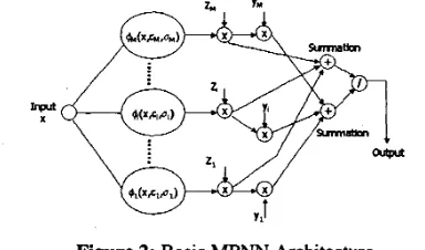
denotes Hermitian operator (or conjugate transpose)Figure 2: Basic MF"N Architecture
The output of each of the kernel functions is real. The complex MPNN equation is the same as the real MPNN equation in [4,5], except that the Hermitian operator is used inside the kernel function instead of a vector transpose operator. The network output is the sum of the product from each center normalized by the sum of the output of the basis function scaled by 2;.
In general, for very small o, the network functions as a nearest neighbor classifier. For a very large number (5,
the network functions as a matched filter.
2.3. Unsupervised Clustering of Centers
The clustering method is similar to the k-means clustering. Close centers that are mapped to the same output are clustered together to form one new center. The location of the new center is the mean of all the centers
being clustered. The total number of centers belonging to this new center is Z,. As a result, a smaller network size can be realized
Learning involves the clustering of centers q and the assignment of an appropriate weight yi and smoothing parameter (3i to each center. A slight variation to Zaknich's clustering technique [9] is used for the positioning of centers.
Define a parameter, Rx, called the radius of influence. Training starts with the first training pair { x i , yi} and establishing a center ci at xi with a corresponding weight of yi. Given n training data pairs, the pseudo-code for the clustering method is as follows:
f o r i = 1: n, if
then
( [ x i
-
qlH[q - q] 5 R,) and (yi(k) = y(k))z,:-
= Z,?'d+
1(Zi
-
1)Cp'd+
x ic y =
zi
z;-
= 1 elseci = xi
end end
3. Center Vector Reduction Algorithm
In the case of channel equalization, as well as many other signal processing applications, the contribution of each center to determining the decision surface varies. In many cases, the decision surface can be represented by a smaller set of selected centers. Without loss of generality, Let us consider binary separations. The two classes are class 1 and class 2.
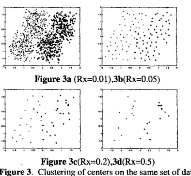
The properties of the radius of influence, Rx, (as discussed in section 2.3) are utilized in the reduction process. As the value of Rx increases, it is observed that the number of centers becomes sparse. As well, the centers from different classes move away from each other. As the gap between the classes widens, the resolution of the decision surface also looses resolution. Figure 3 shows clustering of the same set of two-dimensional input data with varying values of radius of influence, Rx.
Therefore, by choosing only centers closest to the decision surface for varying Rx, we can capture the general form of the decision surface. At the same time the resolution of the decision surface is retained.
The reduction method is as follows:
I 1 1 I
z1 ,' I 0 .
. .
.a I I. , 2 I. I..
0 a 1 t I. *Figure 3a (Rx=O.Ol),3b(Rx=O.O5)
- Figure 3c(Rx=0.2),3d(Rx=0.5)
Figure 3. Clustering of centers on the same set of data with different Rx value.
2. Cluster the training inputs with the first value of R,. 3. Choose randomly p centers from class 1. For each
xpl, find a center from class 2 closest to it. This closest center, cu is the candidate center for the reduced network. Again, for each ce, find a center closest to it belonging to the class 1, ckl.
4. For remaining centers in class 1 that are not Ckl,
select it if the distance to the closest ckl is greater than any center in class 2.
5. Repeat from step 2 and cluster existing centers with the next value of Rx. Stop if all Rx have been tried.
The size of p in step 3 can be arbitrarily selected ranging from 1 to the total number of centers belonging to the same class. The selection of p does not affect greatly the final result. However, choosing extreme values of p (1 or the maximum value) may increase the amount of computation.
The result is a smaller group of centers realizing a decision boundary very similar to the decision boundary of an unreduced network without the requirement of further adaptation of weights.
4. Simulation Results
The channel used in the simulation was sourced from the SPIB database [lo]. The database contains FIR models of different digital microwave radio channel impulse responses. Channel 7 was used. The fractionally sampled factor was taken into consideration. The channel was down-sampled to 32 taps. A further non-linearity characteristic was introduced as follows:
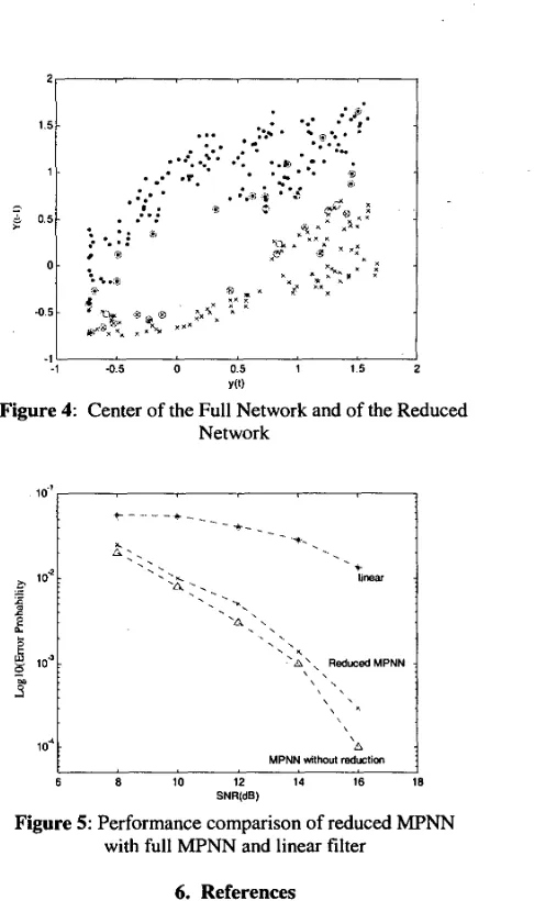
Figure 4 provides a visualization of the centers chosen in the reduced network for the case when the input vector is of dimension two. The centers belonging to the two classes in the full MPNN are marked by dots and crosses. The circles are the centers in the reduced MF"N.
I
SNR(dB)The dimension of the input vectors in figure 5 was four. The non-linear equalizers were trained with 1000 input vectors. The number of centers in both the full network and the reduced network for different signal to noise levels are tabulated in Table 1. The algorithm achieves better than 1/25 reduction for less noisy channels. The reduction ratio for the 8dB signal to noise ratio case was 1/10. The reduction ratio was not as good for noisy cases because the network tried to generalize the noise characteristics. Noise causes regions of the two classes to overlap. More centers were required to generalize the overlapping regions. Generalizing noise is undesirable.
8 IO 12 14 16
The selection of radius of influence, Rx, determines the center reduction ratio and the performance of the reduced network. Generally there is a vague trade-off between the reduction ratio and the performance. In this simulation, The Rx values for the each iteration were [0.01, 0.03, 0.05,1]. The more number of iterations and the smaller the gap between subsequent Rx values, the better the performance of the reduced network.
The result shown in figure 5 indicates that the reduction algorithm slightly degraded the performance from the full MPNN solution. However, the much reduced computational requirement justifies the slight loss in performance.
r'
N U
Centers
I
941 I 936 I 930 I 894 I 863Number of Reduced MPNN I I I I I
I Centei
__- . .- . .
s
I
901
59I
45I
35I
34Table 1. Number of centers in full MPNN and reduced MPNN for different noise level
5. Conclusion
The algorithm has been tested on a realistic high order channel and it has been found that the reduction provides practical implementation for the MPNN. The reduction in network size means faster implementation on a sequential computation machine. Other desirable properties of MPNN such as its fast training and good performance were preserved. The network reduction algorithm offers the MPNN a greater applicability to data analysis problems.
2
-1 -0 5 0 0.5 t 1 5
Y ( 0
Figure 4: Center of the Full Network and of the Reduced Network
10.'
B
Figure 5: Performance comparison of reduced MPNN with full MF"N and linear filter
6. References
[ l ] G.Gibson, S.Siu and C. Cowan, "Multilayer Perceptron Structures Applied to Adaptive Equalisers for Data Communications", in Proc. of ICASSP'89,
pp. 1183-1186, Glasgow, Scotland, May 1989. [ 21 G. Kec hriotis , E .Zervas and E. S. Manolakos, "Using
Recurrent Neural Networks for Adaptive Communication Channel Equalization", ZEEE Trans.
Neural Networks, Vo1.5, N0.2, March 1994.
[3] S. Chen, B. Mulgrew and P.M. Grant, "A Clustering Technique for Digital Communications Channel Equalization Using Radial Basis Function Networks", IEEE Trans. Neural Networks, vol. 4, no.
[4] A.Zaknich, C.deSilva and Y.Attikiouze1, "The Probabilistic Neural Network for Nonlinear Times Series Analysis", in Proc. IEEE Int. Joint Con8
Neural Networks (IJCNN), Singapore, Nov. 1991.
4, pp. 570-579, 1993.
[ 5 ] A. Zaknich, “Introduction to the modified probabilistic neural network for general signal processing applications“, IEEE Transactions on
Signal Processing, Vol. 46, No. 7, pp. 1980-1990, July 1998.
[6] D.F.Specht, “Probabilistic Neural Networks”, Int. Neural Network Soc., Neural Networks, Vo1.3,
[7] D.F.Specht, “A General Regression Neural Network”, IEEE Trans. Neural Networks, V01.2, Nov. 1991.
pp.109-118, 1990.
[8] S.Haykin, Neural Networks: A Comprehensive
Foundation, 2nd Ed, Prentice-Hall, 1999.
[9] A. Zaknich and Y. Attikiouzel, “An unsupervised clustering algorithm for the modified probabilistic neural network, IEEE International Workshop on Intelligent Signal Processing and Communications
Sy;rtems, Melbourne, Australia, pp. 3 19-322, 4-6th
November, 1998.