Owner-manager replacement: a venture capitalist decision model

R E S E A R C H

Open Access

Owner-manager replacement: a venture capitalist

decision model

Robert Cressy

Correspondence:

[email protected]

Birmingham Business School, England, UK

Abstract

We develop a theory of managerial replacement in which a venture capitalist monitors an investee firm run by a manager of unknown quality (Good or Bad). An informative signal Stcorrelated with performance (value-added) is available to the VC at a cost in

each period t. The problem is when to replace him if he underperforms. We derive a solution to this problem that takes the form of an optimal cutoff for each period t, namely,S_tþ1, such that, given his track record, the manager will be replaced if and only if next period’s signal falls belowS_tþ1. The probability of manager replacement is lower for managers with good track records, higher incremental values and lower VC discount rates, and is higher the higher the return to professional replacement, the cost of investment and the costs of monitoring manager performance. Replacement is also predicted to enhance company value.

JEL codes:G24, G32

Keywords:Venture capital; Manager; Replacement; Bayesian learning; Monitoring; Patent

Background

“Cometh the moment cometh the (wo)man”(Anon)

Academics rarely make good managers of high tech businesses and even when they do their usefulness to the company is ephemeral, depending very much on the stage of development the business has reached: for example, a manager useful at startup in product development may have skills that become redundant when full-scale produc-tion and marketing is required (Hellmann and Puri 2002; Wright et al. 2005; Wright and Lockett 2005; Wright et al. 2007). The facts demonstrate that very few first-time entre-preneurs (owner-managers) last the course from inception to maturity; in the first 7 to 8 years of the business’ life, a high proportion are replaced by professional managers (with extensive previous management experience) often at the behest of the venture capitalist or other financier. (Baron et al. 2001; Hellmann 1998; Hellmann and Puri 2002)a. Clearly the replacement decision is an important one both for the entrepreneur and the VC whose investment is tied up in the company. The VC needs someone who is good at managing people (optimising individual performance), who is in touch with the market, the technology and competition (Hellmann and Puri 2002). All these things will influence the business’ performance and ultimately the VC’s returns.

However, when a start-up is run by inexperienced individuals (e.g. academics spinning out from a university science department or other technically-oriented entrepreneurs with little management experience–see Wright et al. 2005, 2007) their quality as execu-tives is (at least initially) unknown. The VC will learn about this quality over time as a result of frequent (or not so frequent) contact with the new company in the form of monitoring and advice (Cumming and Johan 2007). At some point the manager’s ability is sufficiently well known for the VC to be able to make a decision about replacement in favour of a professional manager. This process and its criteria have an inherent eco-nomic logic as we shall shortly see, but the theoretical literature provides little guidance on the matter. Hence the current paper.

In this paper we model the VC learning process and the replacement decision in a Bayesian dynamic programming frameworkb. Briefly, a venture capitalist monitors a start-up run by a manager of unknown quality over a finite horizon. The prob-lem is when to replace him should he underperform. The VC knows that his unob-servable quality as a manager affects the likelihood of an increment to firm value next period, which will ultimately enhance the VC’s return. The VC can however observe an informative signal (e.g. ‘people skills’),c St, of the manager’s ability in

period t at cost c. This enables her to update her prior on the manager’s ability and on the expected profits from retaining him for one more period rather than replacing him with a professional manager. The latter yields a known present dis-counted value to the VC of Πm. In each of the periods we derive an optimal cutoff

St for the signal that results in a rule showing when to replace the manager. The

chances of adding to firm value in any period are predicted to be positively related to past managerial performance (mean value of the signal). The probability of man-ager replacement is thus lower for managers with good track records (S1). We find that it is also lower for managers with higher incremental values (π3(γ2)) and is higher for lower VC discount rates (r). Finally it is higher the higher the return to professional replacement (Π_m), the cost of investment (I2) and the costs of moni-toring manager performance (c).

Basics

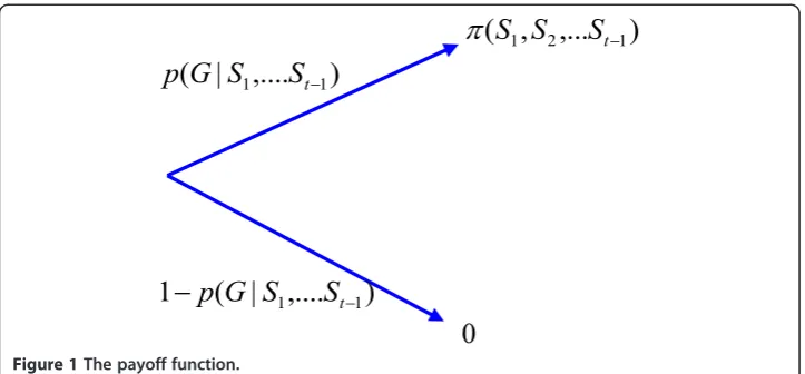
A VC does not know the quality of the manager he employs in his investee company. However, she has a prior distribution on manager quality and judges that the manager is of Good or Bad quality with probability p(G) and p(B) = 1–p(G). Only if the manager is Good is the return to the firm’s project in a period positive. The value of the project at t, if successful, πt, will in general itself depend on the manager’s track record, con-sisting of a set of observable past signals, Sτ;τ¼1;2;…;t−1: Thus we write πt¼π

S1;S2;…St−1

ð Þ(see Figure 1).

Thus the expected value of the project conditional on the information set to date is positive if and only if the manager’s quality is Good.

The VC learning process

signal value, S1. In the next section we develop the optimal value function in terms of these posterior probabilities and the optimal cutoffs associated with them.

The VC can observe a costly signal of the manager’s quality which is either High (H) or Low (L). She thus starts off with a prior on the manager’s quality and then updates this estimate as monitoring occurs. The probability that a manager is Good given a signalS1is by Bayes rule:

p Gð jS1Þ ¼ p S1

jG

ð Þp Gð Þ

p Sð 1jGÞp Gð Þ þp Sð 1jBÞp Bð Þ

ð1Þ

whereS1∈fH;Lg. This can be rewritten as

pðGjS1Þ ¼

1

1þp Sð 1jBÞp Bð Þ p Sð 1jGÞp Gð Þ

ð2Þ

showing more explicitly the dependence of the posterior on the likelihood ratio

p Sð 1jBÞp Bð Þ

p Sð 1jGÞp Gð Þ

ð3Þ

We shall without loss of generality assume in what follows that p Bð Þ ¼p Gð Þ ¼1=2 and that the ratio (3) satisfies the following inequalities:

Assumption 1:

p Hð jBÞ p Hð jGÞ<1<

p Lð jBÞ

p L Gð j Þ ð4Þ

This is equivalent to assuming that the likelihood ratio is increasing in the signal S or that the distribution function for quality Q conditional on H first order stochastically

dominates that of Q conditional on L (see Milgrom (1981) for detailsd). We define for future use the terms x and y:

Definition 1:

x≡p Hð jBÞ p Hð jGÞ; y≡

p Lð jBÞ

p L Gð j Þ ð5Þ

Using Assumption 1 we can conclude thatx<1; y>1 and therefore that

p Gð jLÞ<1

2<p G Hð j Þ ð6Þ

Thus the probability of success (of the manager being Good) in any period, given the signal, is increasing in the value of the signalS2(management performance).

A second observation of the quality signal, S2, results in an updating of the VCs prior to

p Gð jS1;S2Þ ¼

1

1þp Sð 1;S2jBÞ p Sð 1;S2jGÞ

ð7Þ

If observations of the signal are independent this simplifies to

pðGjS1;S2Þ ¼

1

1þp Sð 1jBÞp Sð 2jBÞ p Sð 1jGÞp Sð 2jGÞ

ð8Þ

It follows that the four possible posterior probabilities are related as follows:

p Gð jH;HÞ ¼1=1þx2 ð9Þ

p Gð jH;LÞ ¼p G Lð j ;HÞ ¼1=ð1þxyÞ ð10Þ

p Gð jL;LÞ ¼1=1þy2 ð11Þ

And, using 5:

p Gð jH;HÞ>p Gð jL;HÞ ¼p G Hð j ;LÞ>p G Lð j ;LÞ ð12Þ

Thus a superior‘track record’(sequence of signals) of the manager results in a higher Bayesian estimate of his chances of producing an increment to firm value next period.

Using 5, 9-11 we have

1=1þx2_{>1=ð1þxÞ>1=ð1þyÞ>1=1þy}2 _ð13Þ

so that the dispersion of conditional probabilities of success (value increment) is pre-dicted to increase over time (rounds).

The 2-period optimal value function

The VC has some initial belief about the manager’s quality and updates this measure, St; t¼1;2;…in period t, at a cost. A superior ‘track record’(sequence of past signals) of the manager results in a higher Bayesian estimate of his chances of incrementing value (i.e. generating a positive payoff ) next period.

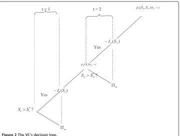
Consider now the value function of the VC in period 2. Figure 2 shows the decision tree structure. Since we have just two periods, the optimal value function will be zero in period 3 and thereafter: EV3¼EV

4¼…¼0. We can therefore write the period 2 VC value function as

V2ðSe2;S1;Þ ¼ max

−I2ðSe2Þþδ½p3ðSe2;S1;Þπ3−c;Πm

ð14Þ

where

I2ðSe2Þ = signal-dependent investment in period 2,I20ðSe2Þ≥0.

δ= discount factor (=1/(1 + r), where r = the risk-adjusted interest rate).

p3ðS2;S1Þ≡pðGjS2;S1Þ = probability manager adds value (is Good) in period 3 given an observed signal about his ability from last period,S1, and the random variable

representing his period 2 signal,Se2.

π3= period 3 value increment of the manager under successf. c = costs of monitoring managerial performanceg.

Πm=present discounted value (p.d.v.) of the VC’s return from the firm under

profes-sional managementh.

The second period value function V2 then shows the present discounted value (p.d. v.) to the VC of either investing and continuing one more period with the existing

man-ager of uncertain quality (yielding p.d.v.−I2ðSe2Þþδ½p3ðSe2;S1;Þπ3−c) or investing and

replacing her with an outsider of known quality (yielding p.d.v. Πm)i. Note that the

continuous signal version of the MLRP guarantees that the first term in the max{.} expression in Equation 14 is increasing in the first period signal S1, since it implies ∂p3ðSe2;S1Þ=∂S1>0.

The expected value of this function with respect to (w.r.t.) S2for anarbitrary cutoff

signalS

^

ES2V2ðSe2;S1jS

^

n

−I2ðSe2Þþδ½p3ðSe2;S1Þπ3−c;Πm o

¼Πm Z

0 S^2

dFðS2jS1Þ þ

Z

S^2

∞

−I2ð Þ þS2 δ½p3ðS2;S1Þπ3−c

dF Sð 2jS1Þ ð15Þ

Choosing the cutoff optimally requires maximising (15) w.r.t. this cutoff and yields the first order condition

−I2 S2 þδ p3 S

2;S1

π3−c

¼Πm ð16Þ

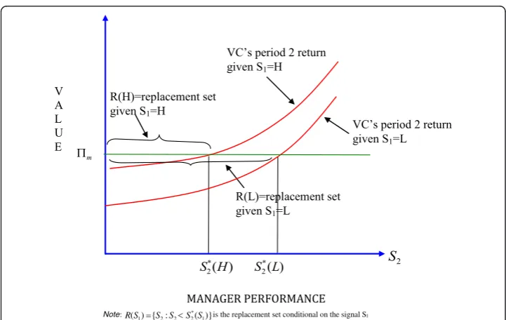
(see Figure 3). The second order condition requires

−I20 S2 þδ π3∂p3 S2;S1

=∂S2>0 ð17Þ

We shall assume henceforth that this condition holdsj. Combining this result with the second order condition for a maximum Equation 3 shows that the VC will at the beginning of period 2 choose to keep the manager if and only if the expected value to the company if he is retained,given his track record(S1), is greater than the value of his replacement. More precisely we have the replacement rule:

Replace the manager in period 2 if and only if

δ½p3ðS2;S1Þπ3−c−I2ð ÞS2 <Πm ð18Þ

where S2is therealisedvalue ofSe2 . Equivalently, we can say that the manager will be replaced, given his initial performance, if and only if his second period performance falls below a certain threshold:

Replace the manager in period 2 if and only if, given S1,

S2<S2 ð19Þ

Plugging 3 into 2 the optimal period 2 value function now becomes

ES2V

2ðSe2;S1Þ ¼Πm ð20Þ

whereES2V

2ðSe2;S1Þ≡maxS2ES2V2ðSe2;S1S2Þ.

We now let the manager’s incremental value, π3(γ2), be increasing in a market de-mand parameter γ2. Consider the continuous signal case. Using the MLR property of the distribution function we get

∂p2 ∂S1>

0 ð21Þ

Differentiating w.r.t. the various parameters we then get the following comparative static results:

∂S2 ∂S1;

∂S2 ∂γ2

;∂S2

∂δ <0 ð22Þ

∂S2 ∂Πm;

∂S2 ∂η2

;∂S2

∂c >0 ð23Þ

where ηis a shift parameter in the function I2(I2η>0Þ. Thus we have shown that in

the second period the probability of manager replacement is lowerfor managers with good track records(S1), higher incremental values (π3(γ2)) and lower VC discount rates

(r), and that it ishigherthe higher the return to professional replacement (Π_m), the cost of investment (I2) and the costs of monitoring manager performance (c). Figure3

illus-trates the effects of better performance on the likelihood of manager replacement. We move back now to period one. The period 1 value function is given by

V1ðSe1Þ ¼ max

−I1ðSe1Þþδ½p2ðSe1Þπ2ðSe1Þ−cþES2V2ðS1;eS2Þ;Πm

ð24Þ

with expected value

ES1V1ðSe1Þ ¼ES1max

−I1ðSe1Þþδ½p2ðSe1Þπ2−cþES2V2ðSe2;Se1Þ;Πm

¼Πmþ

Z

S^1

∞

−I1ðSe1Þþδ½p2ð ÞS1 π2−cþES2V2ðSe2;Se1Þ

dF Sð Þ1

ð25Þ

Choosing the period 1 cutoff optimally requires

−I1ðSe1Þ þδ½p2 S1 π2þES2V2ðSe2;S

Substituting back into Equation 11 theoptimalperiod 1 value function now becomes

ES1V

1ðSe1Þ ¼Πm ð27Þ

It is clear that whilst the optimal value function is a constant the optimal cutoffs will vary with the information available at the time. The comparative statics of the first period cutoff with respect to the relevant parameters, assuming symmetrically that π2=π2(γ1) is increasing in the demand parameter,γ1, show that, as might be expected, the first period probability of manager replacement is lower for managers with good track records(S1), higher incremental values (π3(γ2)) and lower VC discount rates (r); it ishigherthe higher the return to professional replacement (Π_m), the cost of investment (I2) and the costs of monitoring manager performance (c)k.

The T-period model

The generalisation of the model to T periods is straightforward and we present most of the results rather than proving them in the text. The obvious way to represent the manager’s track record in the multiperiod context is by the mean of the signals over the periods up to the present (t). For some distribution functions (e.g. the Normal) the mean of the signal history and the number of periods before the present, t-1, will be a sufficient statistic for the signal historyl. Restricting ourselves to such distributions we can write the tthperiod value function as

VtðSet;St−1Þ ¼ max −ItðSetÞþδ½ptðSet;St−1Þπtþ1−cþEStþ1Vtþ1ðSe tþ1;St−1Þ;Πm

ð28Þ

where

St¼

Xt

i¼1

Si=tis the mean signal from the manager up to time tm.

Taking expectations with respect to the period t signal we get

E_S˜_tVt S˜t;

St−1

¼E_S˜_tmax

(

−It S˜t

þδ ptþ1

St−1

h

πtþ1−cþE_S˜ tþ1Vtþ1

˜ Stþ1;

St

;Πm )

¼ΠmF S^t þ Z∞ ^ St (

−It S˜t

þδ

½

St−1

πttþ1−cþE_S˜ tþ1Vtþ1

˜ Stþ1;

St i)

dF Sð Þt

ð29Þ

Differentiating w.r.t. the tthperiod cutoff we get the optimality condition

−It St þδ½ptþ1 St;St−1

πtþ1−cþEStþ1Vtþ1ðSetþ1;S

tÞ ¼Πm ð30Þ

where we define

St ¼t−1 S

t þðt−1ÞSt−1

ð31Þ

We have using the MLR property that the probability of success increasing in the manager’s track record:

∂pt

∂St−1

>0 ð32Þ

Comparative statics then go through as before withS1being replaced bySt−1:

∂St

∂St−1

;∂St

∂γt

;∂St

∂δ <0 ð33Þ

∂S_t

∂Πm;

∂S_t

∂η_t; ∂S_t

∂c >0 ð34Þ

Summary and conclusions

We developed a theory of managerial replacement in which a venture capitalist moni-tored an investee firm run by a manager of unknown quality (Good or Bad). An in-formative signal Stcorrelated with performance (value-added) was available to the VC at a cost in each period t. The problem was when to replace him if he underperformed. We derived a solution to this problem that took the form of an optimal cutoff for each period t, namely,Stþ1, such that, given his track record, the manager would be replaced if and only if next period’s signal fell below Stþ1. We showed that the probability of manager replacement was lower for managers with good track records, higher incre-mental values and lower VC discount rates, and was higher the higher the return to professional replacement, the cost of investment and the costs of monitoring manager performance. Replacement was also predicted to enhance company value.

Endnotes a

Hellmann, reports statistics from Hannan et al. (1996) who found that in Silicon Valley high tech startups 20% of owner-managers were replaced in the first 10 months of the business’life, rising to 80% in the first 80 months. These figures we shall see later are broadly consistent with those in the current dataset.

b

There is a parallel here with the model of entrepreneurship as a learning experiment in Jovanovic (1982). Jovanovic argues that an entrepreneur learns about his ability in entrepreneurship only by starting a business. His initial prior is updated by successive feedback from the market on his costs of operation. Our model is consistent with this view of the entrepreneur, but we look at it from the VCs perspective, so that the VC learns about the entrepreneur’s ability by investing in him or her and observing her performance. In Jovanovic the entrepreneur decides if and when to quit based on her updated information on her skills; in our model the VC makes the decision for her.

c

A great manager has the ability to bring out the very best in people thus optimising their ability. This is modelled in the paper by assuming that the probability of success in any period increases in the value of the signal.

d

Very briefly Milgrom shows that under the Monotone Likelihood Property (hence-forth MLRP) given in our case by inequalities 4, that any risk averter (in our case the VC) will strictly prefer the posterior distribution manager quality Q (in our case B, G) conditional on the signal H over the same distribution conditional on L.

e

See Milgrom (1981). f

We shall henceforth, without loss of generality, drop the dependence ofπon the sig-nals St.

g

h

We assume that this return is based on a known success probability (no learning needs to take place on the part of the VC about the parameters).

i

Note that we are modelling only stages at which investment by the VCoccurs. There is always in practice the possibility that the VC will not invest at all at a given stage. However, our data (as most other data) records only stages at which investment oc-curred. Hence our tests will be on‘superior’businesses in this sense. Our modelling ef-fectively assumes therefore that the value function in 1 is positive with probability 1. It is very straightforward to adjust the model to take into account the possibility of no in-vestment at a given stage.

j

It is automatically satisfied, given the MLRP, ifI02 ¼0. k

Note that because of the absence of observations on the managerial signal in period 1 (this is not visible until period 2) we cannot examine the impact of track record at this stage.

l

We can assume that the signals H and L assume the values 1 and 0 respectively. This gives us as the mean value the proportion of past periods in which the manager per-formed well.

m

Bear in mind here that this mean contains now therandomvariableSe_tof period t.

Competing interests

The author declares that he has no competing interests.

Received: 16 June 2013 Accepted: 3 October 2013 Published: 7 July 2014

References

Baron, J, Hannan, M, & Burton, MD. (2001). Labor pains: change in organisational model and employee turnover in young, high-tech firms.American Journal of Sociology, 106(4), 960.

Cumming, D, & Johan, S. (2007). Advice and monitoring in venture finance.Financial Markets and Portfolio Management, 21(1), 3–43.

Hannan MT, Burton MD, Baron IN. (1996). Inertia and Change in the Early Years: Employment Re-lations in Young, High-Technology Firms.Industrial and Corporate Change5:503–535.

Hellmann, T. (1998). The allocation of control rights in venture capital contracts.Rand Journal of Economics, 29(1), 57–76. Spring.

Hellmann, T, & Puri, M. (2002). Venture capital and the professionalization of start-ups: empirical evidence.Journal of Finance, 57, 169–197.

Jovanovic, B. (1982). Selection and the evolution of industry.Econometrica, 50(3), 649_–670.

Milgrom, P. (1981). Good and bad news: representation theorems and applications.Bell Journal of Economics,. Wright, M, Chapple, W, Siegel, D, & Lockett, A. (2005). Assessing the relative performance of UK university technology

transfer offices: parametric and non parametric evidence.Research Policy, 34, 369–384.

Wright, M, & Lockett, L. (2005). Resources, capabilities, risk capital and the creation of university spin-out companies. Research Policy, 34, 1043–1057.

Wright, M, Siegel, D, & Veugelers, R. (2007). University commercialization of intellectual property: policy implications. Oxford Review of Economic Policy, 23(4).

doi:10.1186/2251-7316-2-5