Deep Latent Generative Models for Energy Disaggregation

(1)

The Thirty-Third AAAI Conference on Artificial Intelligence (AAAI-19)

Deep Latent Generative Models for Energy Disaggregation

Gissella Bejarano

David DeFazio

Arti Ramesh

Abstract

Thoroughly understanding how energy consumption is dis-aggregated into individual appliances can help reduce house-hold expenses, integrate renewable sources of energy, and lead to efficient use of energy. In this work, we propose a deep latent generative model based on variational recurrent neu-ral networks (VRNNs) for energy disaggregation. Our model jointly disaggregates the aggregated energy signal into in-dividual appliance signals, achieving superior performance when compared to the state-of-the-art models for energy dis-aggregation, yielding a29% and41% performance improve-ment on two energy datasets, respectively, without explicitly encoding temporal/contextual information or heuristics. Our model also achieves better prediction performance on low-power appliances, paving the way for a more nuanced dis-aggregation model. The structured output prediction in our model helps in accurately discerning which appliance(s) con-tribute to the aggregated power consumption, thus providing a more useful and meaningful disaggregation model.

Introduction

Designing machine learning models for smart energy con-sumption is an important research problem, having a tremen-dous impact on society. A crucial sub-problem in facil-itating smart energy consumption is being able to accu-rately disaggregate energy signals into their component appliance signals. This process is also known as energy disaggregation/non-intrusive load monitoring (NILM). This exercise provides residents with an accurate view and un-derstanding of their energy consumption and can potentially help in reducing the peak energy consumption and facilitat-ing efficient usage and conservation of energy. Recent ad-vances in variational inference for deep learning have re-sulted in more expressive deep generative models such as variational auto-encoders (VAEs) and variational recurrent neural networks (VRNNs) that possess the ability to encode continuous latent variables. These latent variables provide the models with a powerful layer of abstraction that captures the variations in the input data and helps in generating the output data. These models map the input sequence into con-tinuous latent variables using an inference network (referred

to as an encoder), and then use the generative network (re-ferred to as a decoder) to reconstruct the input sequence by sampling from the latent variables. Chung et al. (2015) pro-pose variational recurrent neural networks (VRNNs), which extend VAEs to model sequences by introducing high-level latent variables in RNNs. Deep generative models such as VRNNs and VAEs have achieved state-of-the-art perfor-mance in many sequence-to-sequence language tasks such as machine translation, paraphrase generation, and textual entailment, but have not been explored for the problem of energy disaggregation.

In this work, we present a novel deep generative architec-ture for disaggregation that leverages and adapts VRNNs to jointly disaggregate the total energy consumption into indi-vidual component appliance signals. Our proposed approach learns the abstraction of the aggregated energy consumption over latent variables at training time and then generates all the individual appliance signals jointly by sampling from the latent variables at test time. Hence, at test time our model only depends on the aggregated signal and the latent vari-able abstractions learned during training and does not de-pend on contextual information and appliance data from pre-vious time steps, making it a meaningful model for energy disaggregation.

Specifically, we make the following contributions:

1. We present a novel deep generative architecture for per-forming sequence-to-many-sequence prediction (aggre-gated consumption to appliance consumptions) needed for energy disaggregation by leveraging and adapting variational recurrent neural networks (VRNNs). Our model generates continuous power consumption signals as opposed to state-of-the-art approaches that model con-sumption through discrete appliance states.

2. We model the structure among the different appliances in a household by jointly predicting each of them at the same time from the aggregated signal. We cast the different ap-pliance energy signatures as a structured prediction prob-lem, modeling the structure among the different appliance energy consumption signals over time, to effectively rep-resent and reason about their dependence.

(2)

state-of-the-art energy disaggregation approaches that use exten-sive additional past temporal and contextual information (Tomkins, Pujara, and Getoor 2017; Shaloudegi et al. 2016). Further, our model achieves a superior prediction performance on low power consuming appliances, which are harder to predict and are often ignored by most exist-ing approaches.

4. Through qualitative analysis, we demonstrate that our models can achieve a superior disaggregation for both high and low energy consumption states and accurately discerns which appliance(s) contribute to the aggregated power consumption, thus providing a more useful and meaningful disaggregation model.

5. We demonstrate the extensibility of our model in predict-ing individual appliance consumption on previously un-seen data by testing on a building that is left out while training. We observe that our model achieves a superior prediction performance on two buildings in REDD, thus making it potentially extensible to new datasets.

Related Work

Hart et al. (Hart 1992) was the first to introduce the prob-lem of energy disaggregation. Perhaps the most popular approach for energy disaggregation is using factorial hid-den Markov models (FHMMs) (Ghahramani and Jordan 1997), which generalize HMMs by using a distributed rep-resentation and its variants (Kim et al. 2011; Kolter and Jaakkola 2012; Parson et al. 2012; Johnson and Willsky 2013). Shaloudegi et al. (2016) propose a scalable algo-rithm for this problem that extends FHMMs. Supervised machine learning models such as Support Vector Machines (SVMs) and k-Nearest Neighbors (k-NNs) and unsupervised models that use prior appliance models have also been ap-plied to this problem (Altrabalsi et al. 2016; Barker 2014; Faustine et al. 2017; Makonin et al. 2016). Some other mod-els have relied on other information apart from the aggre-gated consumption to model relationships with user’s be-havior and climate (Li and Zha 2016; Tomkins, Pujara, and Getoor 2017; Zhong, Goddard, and Sutton 2015). Tomkins et al. (2017) propose a structured probabilistic framework for energy disaggregation. Recent advances in deep learn-ing have spurred deep-learnlearn-ing based energy disaggrega-tion models (Kelly and Knottenbelt 2015; Lange and Berg´es 2016; Barsim, Mauch, and Yang 2018; do Nascimento 2016; Zhang et al. 2018; Huss 2015; Batra et al. 2018).

In this work, we propose a deep latent generative model based on VRNNs that combines the advantages of the mod-eling complexity of deep neural networks and the rich rep-resentational power of latent variables in probabilistic mod-els such as FHMMs. Our model learns to predict all indi-vidual appliance signalsjointlyfrom the aggregated signal. We compare our approach to two recent state-of-the-art ap-proaches for energy disaggregation: a) ADMM-RR, a scal-able variant of FHMMs (Shaloudegi et al. 2016), and b) Tomkins et al.’s (2017) joint probabilistic approach to en-ergy disaggregation, and show that our approach achieves superior prediction performance.

Deep Latent Generative Models for

Energy Disaggregation

In this section, we describe the energy disaggregation prob-lem and the suitability of VRNNs for the same. Then, we present our deep latent generative energy disaggregation ar-chitecture.

Energy Disaggregation Problem

The problem of disaggregation is to calculate the en-ergy consumption of individual component appliances given the total aggregated power consumption. Let x =

(x1, x2, ..., xT) be the aggregated energy consumption of

a house over T time steps, where xt ∈ R+. Let I be the

number of appliances. The individual energy consumption of appliance i is denoted by yi _{= (}_yi

1, y2i, ..., yiT), where yi

t ∈ R+. Consequently the aggregated energy signal at a

given time can also be expressed asxt=P I

i=1y

(i)

t . We use ytto denote the consumption timet for all the appliances: yt = {y1t, y2t, ..., ytI}.Our goal in this work is to develop a deep latent generative energy disaggregation framework that can learn to infer the continuous-valued appliances’ consumption given the aggregated energy consumption.

Variational Recurrent Neural Networks

Variational Recurrent Neural Networks (VRNNs) (Chung et al. 2015) are a recently developed deep neural network ar-chitecture that introduce latent variables and temporal de-pendencies between them in the different time steps in the RNN architecture. The core of a VRNN is a vari-ational auto-encoder (VAE) (Kingma and Welling 2014; Rezende, Mohamed, and Wierstra 2014). VAEs and VRNNs are variants of autoencoders (AE) and recurrent neural net-works (RNNs) that encode latent variables and probabilistic transition functions. The principal difference between VAE and VRNN is that VRNN models the dependencies between latent variables across subsequent time steps, thus providing us with the ability to accurately abstract highly non-linear dynamics in sequential data. Since the prior distribution at timesteptis dependent on all the preceding inputs via the RNN hidden stateht−1, the introduction of temporal

struc-ture in the prior distribution is expected to improve the rep-resentational power of the model. We first discuss the suit-ability of VRNNs for the energy disaggregation problem and then present our deep generative architecture.

(3)

Energy consumption signals are highly structured, i.e., they have a high signal to noise ratio; the variations in the data are due to signal itself rather than noise. Thus, the pres-ence of structured output functions in VRNNs along with their ability to represent complex non-linear data make them ideal for modeling this domain.

The structured output functions present in VRNNs aid the joint prediction of disaggregated appliance signals from the aggregated consumption. Kelly et al. (2015) use RNNs for the energy disaggregation problem, but their model does not disaggregate all appliance signals at once. Instead, they train a separate model for each appliance. Due to the lack of probabilistic transitions between latent variables and struc-tured output functions, this approach fails to capture the de-pendencies between the different appliance signals and thus lacks the ability to accurately identify the contributing ap-pliance signals in an aggregated signal.

In the energy disaggregation problem, usually power con-sumption is mapped to discrete appliance states (Shaloudegi et al. 2016; Tomkins, Pujara, and Getoor 2017). This, how-ever, ignores the fine-grained variations in the signals. The deep structured construction of our model and the presence of latent variable abstractions and probabilistic transitions between them provide us with the ability to model the ex-act consumption of appliances as continuous values and de-tect fine-grained variations in the signals. Since we do not approximate signals into consumption states and model the exact continuous values, our approach requires minimal pre-processing and is able to model these minute variations.

VRNN-DIS-ALL: A Deep Generative Energy

Disaggregation Framework

We bring out the modeling power of VRNNs by adapt-ing them to disaggregate individual appliance signals jointly from the aggregated power consumption signal. In the fol-lowing sections, we present the generative process, infer-ence, and learning in our model, VRNN-DIS-ALL. We also highlight the adaptations to the original VRNN for the energy disaggregation problem.

Generation The VRNN contains a VAE in each time step but the prior on the latent variable follows a distribution that is conditioned on the hidden state at timet−1,ht−1. We

augment the prior distribution to include bothht−1and the

aggregated consumption at timet, denoted byxt. Hence, the

random variableztfollows the distribution:

zt∼N(µ0,t, diag(σ0,t2 )) (1)

where,[µ0,t, σ0,t]denote the parameters of the distribution φprior_τ (ht−1, xt). While for the generation task described in

Chung et al. (2015), the prior distribution only depends on

ht−1, we adapt it to include the aggregated signal as we are

interested in generating the disaggregated appliance signal from the aggregated signal. Next,yt(disaggregated signal)

is generated givenztandht−1from the distribution:

yt|zt∼N(µy,t, diag(σy,t2 )) (2)

where, [µy,t, σy,t] = φdecτ (φzτ(zt), ht−1). Chung et al.

(2015) note thatφpriorτ andφdecτ can be any highly

flexi-ble functions and are essential for learning complex depen-dencies. In our models,φprior

τ andφdecτ are neural networks

with one-hidden layer with standard activation functions. The hidden layer has a hyperbolic tangent (tanh) and the output layers forµy,tandσy,thave linear and softplus

ac-tivations, respectively. The RNN hidden state calculation is given by

ht=f(φxτ(xt), φyτ(yt), φzτ(zt), ht−1) (3)

where, f is the transition function between hidden states. The feature extractors,φx

τ,φyτ(yt), andφzτ, can be any

ex-pressive function. We use a 1-hidden layer neural network for the same. The learning problem is to learn the prior dis-tribution,φpriorτ (ht−1, xt), to be as close as possible to the

approximate posteriorφenc

τ (φxτ(xt), φyτ(yt), ht−1).

Inference At training time, VRNN works as an encoder, learning the approximate posterior as a function of xt,yt

andht−1.

zt|xt, yt∼N(µz,t, diag(σ2z,t)) (4)

where,[µz,t, σz,t]denote the parameters of the distribution

φenc

τ (φxτ(xt), φyτ(yt), ht−1). In addition to the feature

ex-tractors fromxtandzt, we also includeφyτ(yt)that extracts

the features of the disaggregated signalytat training time.

Inference at training time is done by samplingztfrom this

approximated posterior distribution. At test time,ztis

sam-pled from the learned prior distribution that is learned during training. This difference in theztcan be appreciated in

Fig-ure 1 where we can see how the distributionφprior

τ replaces

the encoder distributionφencτ .

Learning Learning is performed by minimizing the sum of two components: distance between the posterior and the prior distribution and the log-likelihood of the output. In the first term in Equation 5, we minimize the Kullback-Leibler divergence distance (KL divergence) between the approx-imate posterior in Equation 4 (denoted by q in Equation 5) and the prior distribution (denoted bypin Equation 5), whereztdepends only on aggregated signal (x≤t) and the

latent variable states at previous time steps (z < t). The sec-ond term captures the negative log-likelihood of the output distribution from which we sampleyt.

KL(q(zt|x≤t, y≤t, z < t)||p(zt|x < t, z < t))

+logp(yt|z≤t, x < t) (5)

Training At training time, our goal is to learn an approxi-mate function that is very similar to the conditional distri-bution p(z|y) by minimizing the KL divergence between the prior distribution (φprior

τ ) and the approximate

poste-rior or the encoder distribution (φencτ ) (Figure 1a). We

(4)

or from the predictions generated by the model (ˆyt). In our

models, we use an inverse sigmoid decay. It is defined as:

pi =k/(k+exp(i/k))

where,pi is the sampling probability andk >= 1gives

the speed of convergence. This probability is calculated at each time step.

...

(a) VRNN-DIS-ALL at training

...

(b) VRNN-DIS-ALL at test

Figure 1: Graphical illustrations of VRNN-DIS-ALL train-ing to reconstruct disaggregated appliance signals from the aggregated and disaggregated signals and as a generative model of disaggregated appliance signals from only the ag-gregated signal at test time.

Testing At test time, we only input the aggregated en-ergy consumption information xt. We no longer use the

encoder distribution but the parameters of the learned prior distribution to sample the latent variables zt, i.e.,

zt ∼ N(µ0,t, diag(σ20,t)). Then, we calculate the

param-eters of the distribution of each appliance using yti|zt ∼ N(µi

y,t, diag(σy,ti 2

)), where [µi

y,t, σy,ti ] is now calculated

from the learned prior distribution. We calculate the next recurrent hidden layerhtas a function of feature extractor

neural networks forxt,yˆt, andzt, and previous hidden state ht−1, i.e., f(φxτ(xt), φτz(zt), φyτ(ˆyt), ht−1). Note that here

we use the predictedyˆinstead of the actualy(Figure 1b).

Implementation Details We develop our model1 _{on the}

original VRNN implementation (Chung et al. 2015) in Theano. Figure 2 captures the model architecture. It shows the different hidden layers, number of nodes in the hidden layers, identifies the components corresponding to the hid-den layer, and captures the interactions between them for one iteration of training from time t −1 to t. The name of each component and the activation function applied to nodes in that hidden layer is mentioned at the top and the number of nodes is indicated in the bottom of each hidden layer. The architecture shows the distribution from wherezt

will be sampled at training time (from the encoder, marked in green) and at inference/test time (from the prior, marked in red). The weight matrices of all layers are randomly ini-tialized using a uniform distribution. The LSTM-cell diago-nal matrix that captures the interaction between the recurrent

1

https://bitbucket.org/gissemari/disaggregation-vrnn

(ReLU)

{1}

{I} {200}

{200} (ReLU)

(tanh) (tanh)

{200} {150} {150}

(ReLU)

{500} (softplus)

(linear)

{100} {100}

{100}

(ReLU) (ReLU)

{500} (softplus)

(linear) {100}

{100}

. . .

(ReLU)

(ReLU/ linear)

(softmax)

(softplus) {200}

{20}

{20} {20}

{20} {1}

{1}

. . .

Figure 2: Architecture of the VRNN-DIS-ALL model. Solid lines represent fully connected layers and dashed lines rep-resent the sampling process.

statesht−1andhtis initialized randomly from a normal

dis-tribution ensuring its orthogonality. The initial hidden state of the recurrent neural network is initialized to0.

We experiment with different activation functions forθµ

and find that ReLU activation function for θµ works

bet-ter for some buildings while for others the linear activation function works better. Forθσandcoef1, we apply asoftmax

andsoftplusactivation functions, respectively. These

param-eters are calculated for each appliance, so the final layer has as many Gaussian mixture models (GMMs) as appliances.

Experimental Evaluation

We conduct experiments to answer the following questions:

1. How well do our deep generative models perform in en-ergy disaggregation?

2. Are our models able to effectively identify which appli-ance(s) are contributing to the aggregated consumption?

Model Disaggregation

Representation

Temporal

Dependencies

Context/

Heuristics

ADMM-RR(Shaloudegi et al. 2016) Discrete states Encoded X

INTERVAL(Tomkins et al. 2017) Discrete states Encoded X

INSTANCE(Tomkins et al. 2017) Discrete states Encoded X

CONTEXT(Tomkins et al. 2017) Discrete states Encoded X

VRNN-DIS-ALL(our approach) Continuous Learned 7

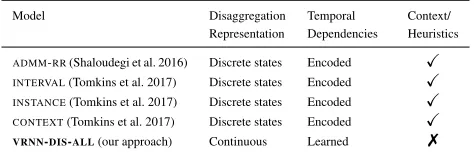
Table 1: A comparison table between our model and the state-of-the-art energy disaggregation approaches

(5)

b) Interval, Instance, and +Context models from Tomkins et al. (2017). Table 1 gives a comparison of our approach with the state-of-the-art energy disaggregation models. Our approach uses a continuous value representation, does not explicitly encode any domain-specific variables or capture any dependencies among them, and does not require any ad-ditional contextual information (such as temperature of the day, day of the month/year, user-specific contextual infor-mation). Our model automatically learns these dependencies from training data. In our experiments, we demonstrate that our models outperform ADMM-RR across most appliances in both the datasets and outperforms Tomkins et al.’s best model on one dataset and achieves comparable performance on another despite using no temporal, domain-related, or contextual information.

We present two metrics of evaluation for both the datasets: i) mean absolute error (MAE), and ii) percentage of total energy estimated by each appliance compared to percentage of total energy in the original data. The MAE is calculated by computing the absolute value of the difference between the predicted disaggregated appliance consumption (yˆt) and

the actual consumption (yt). Percentage of energy estimated

is calculated by taking the ratio of predictions associated with the appliance to original aggregated signal. This per-centage is compared with the actual perper-centage of energy consumption of the appliance in the aggregated energy con-sumption. We evaluate our percentage predictions in the fol-lowing ways: i) first, we compare the actual percentage num-bers between our predictions and the actual data, ii) second, we compute the percentage/range of error between the pre-dicted and the actual by taking the ratio of the difference in the percentages with the actual percentage, and iii) third, we compare our deviation in percentages (percentage of error) to the deviation in percentages reported for the same build-ing by Tomkins et al.

Datasets

We evaluate our model on two real-world energy datasets: i) Pecan Street Inc. Dataset (DATAPORT) (dat 2016), and ii) Reference Energy Disaggregation Dataset (REDD) (Kolter and Johnson 2011). These datasets have been used in sev-eral previous works (Tomkins, Pujara, and Getoor 2017; Shaloudegi et al. 2016; Makonin et al. 2016).

DATAPORT The Pecan Street dataset (DATAPORT) con-sists of energy consumption readings at 1-minute and 1-hour intervals. We evaluate on the finer-grained 1-minute read-ings. As there are missing values, we work on the same subset of buildings (2859, 3413, 6990, 7951, 8292) that Tomkins et al. (2017) use in their work. We consider data for the following appliances: air conditioner, furnace,

refrig-erator, dishwasher, kitchen outlet, dryer, microwave, and

clothes washer.

REDD The REDD dataset contains data for 10 houses from the greater Boston area for approximately two months. We again consider the same five houses (houses1,2,3,4, and6) that Tomkins et al. (2017) and Makonin et al. (2016) consider so that we can make a fair comparison. We also consider the same four appliances for houses1,2, and3:

refrigerator,dishwasher,light,microwave. For house6we

excludemicrowaveas the data for that appliance is unavail-able. We use the non-intrusive load monitoring toolkit (Batra et al. 2014) to get a sampling rate of every 6 or 60 seconds.

Data Preprocessing

To preprocess the data for our model, we first determine the minimum activation threshold for each appliance in each dataset. Then, we use a non-overlapping sliding window on the entire original time series data to construct sequences of fixed length from them. From these sequences, we filter the ones where at least one data point in the sequence is greater than the minimum threshold activation for each appliance. We treat each sequence as one data instance. We split the to-tal number of instances into training, testing, and validation sets in the ratio 50%:25%:25%, respectively. We record the performance metrics in the validation set every ten epochs to detect and prevent overfitting.

We construct batches of instances (which we refer to as

mini-batch) and train the model for many epochs for each

mini-batch. This enables the model to see a smaller num-ber of instances for a longer training period, enabling it to model the structural dependencies in the data. We use5-30 mini-batches. We report the average scores from three differ-ent train-test-validation splits across both datasets. Note that our approach uses very minimal pre-processing and domain knowledge when compared to the existing state-of-the-art approaches.

Energy Disaggregation Results on D

ATA

P

ORT

Table 2 shows the MAE of each appliance in each build-ing in DATAPORTdataset. Our model is able to achieve low MAE for appliances that consume higher energy in average such as clothes washer and air conditioner. The first one shows a MAE of1.5,6,8.5, and2.5in buildings2859,6990, 8292and3413, respectively and theair conditionerobtains a MAE of9.5for building2859. In addition to that, appli-ances which consume less energy on average such as

dish-washer,kitchen appliance, andmicrowaveshow an average

MAE of less or equal than15.5among all buildings. It is in-teresting to note that Tomkins et al.’s prediction performance of appliance states for appliances that consume lesser power on average and are intermittent is lower as indicated by their lower values of precision, recall and F1 scores. Thus, our model is able to discern patterns of consumption in both kinds of appliances and hence perform a more accurate dis-aggregation.

Figure 3a shows the comparison of average MAE value across the buildings and appliances between our model VRNN-DIS-ALL and two existing state-of-the-art ap-proaches. Since we consider the same set of buildings and appliances, we make a direct comparison to the results pre-sented by Tomkins et al. (2017). We observe that our model achieves29% performance improvement in MAE over the

+CONTEXT model (Tomkins et al.’s best model) and 41%

(6)

Building

Appliance 2859 6990 7951 8292 3413 AVG/Appliance

Air 9.50 199.50 152.50 98.50 64.00 104.80

Furnace 40.50 110.50 59.00 56.50 32.50 59.80

Refrigerator 32.50 70.00 77.50 60.00 71.50 62.30

Clothes washer 1.50 6.00 24.00 8.50 2.50 8.50

Dryer 4.00 52.00 33.00 78.50 35.50 40.50

Dish washer 1.00 8.00 14.50 25.00 9.50 11.60

Kitchenapp 1.00 3.00 14.00 17.50 1.00 7.30

Microwave 10 .00 12.50 40.00 9.00 6.00 15.50

AVG/Building 12.50 57.69 51.81 44.13 27.81 38.79

Table 2: VRNN-DIS-ALL results on DATAPORTshowing the MAE for each appliance for the five buildings.

in extracting complex features and learning structural de-pendencies among them. This eliminates the necessity to en-code domain-specific information and their relationships as in existing probabilistic energy disaggregation approaches. Hence, our approach requires less manual effort and can scale easily to new datasets without the need for careful en-coding of graphical structure among variables.

VRNN-DIS-ALL Instance Interval +Context ADMM-RR 0

20 40 60 80

Mean Absolute Error (KWatts)

(a) MAE: DATAPORT

Microwave Dishwasher Refrigerator Lights All 0

10 20 30 40 50 60 70

Mean Absolute Error (KWatts)

VRNN-DIS-ALL Instance Interval ADMM-RR

(b) MAE: REDD

Figure 3: MAE comparing our proposed model VRNN-DIS-ALL with existing state-of-the-art models (Interval, Instance, +Context, and ADMM-RR)

Figure 4 gives the percentage of total energy consumed by the appliance as predicted by our model compared with the actual percentage of total energy consumed by the appli-ance in the original data. We group the appliappli-ances intoair

conditioner(air),furnace,refrigerator,dryer, andothers, to

enable an easy comparison to Tomkins et al.’s percentage calculations. Comparing the predicted percentage of total energy with the actual forair conditioner across all build-ings, we observe that our model predicts within 4% of the actual percentage of energy consumed by the appliance for 4out of5buildings. Similarly, fordryer, our model’s predic-tions lie within 11% for4out of5buildings, and forfurnace, our model’s predictions lie within 6% for3out of5 build-ings. Comparing the percentages for building3413with the percentages reported by Tomkins et al., we observe that our model’s percentage prediction for air conditionerdeviates by only3.6% from the actual percentage, while theirs

de-viates by 7.3%. Similarly, comparing the percentages for

furnacewe observe that ours deviates by1.5% while theirs

deviates by10%. For the rest of the appliances, our model achieves comparable differences in percentages between the predicted and the actual values to their model.

Building 2859

0 0.25 0.5 0.75

Building 6990

0 0.25 0.5 0.75

Building 7951

0 0.25 0.5 0.75

Percentage of Total Energy Consumption

Building 8292

0 0.25 0.5 0.75

Building 3413

Air Furnace Refrigerator Dryer Others

0 0.25 0.5 0.75

Real Predicted

Figure 4: Percentage of total energy consumption of each appliance for Dataport homes

Energy Disaggregation Results on REDD

Figure 3b gives the comparison for average MAE of each appliance across buildings between VRNN-DIS-ALL and existing state-of-the-art approaches. Here, we only compare againstINTERVALand INSTANCEmodels from Tomkins et al. as the +CONTEXTmodel cannot be used due to absence of contextual information in the dataset. We observe that our model achieves superior performance ondishwasherand

lights, which are harder to predict due to their

unpredictabil-ity. We get performance improvements of 69% and 68%, re-spectively, over ADMM-RR and56% for dishwasher over Tomkins et al. For the other appliances:microwaveand

re-frigerator, we achieve comparable performance to one of

the existing approaches. Comparing our overall MAE aver-aged over all buildings and all appliances with ADMM-RR, we observe that VRNN-DIS-ALL achieves a performance improvement of 41%. Our overall MAE is comparable to Tomkins et al.’s models, despite having no careful encoding of domain-specific temporal, contextual, and structural de-pendencies using graphical templates, paving the way for a model that can be extended easily to other settings.

(7)

Building 1

0 0.15 0.3 0.45 0.6 0.75

Building 2

0 0.15 0.3 0.45 0.6 0.75

Percentage of Total Energy Consumption

Building 3

Refrigerator Dish Washer Light Microwave

0 0.15 0.3 0.45 0.6 0.75

Building 6

Refrigerator Dish Washer Light

0 0.15 0.3 0.45 0.6 0.75

Real Predicted

Figure 5: Percentage of total energy consumption of each appliance for REDD homes

an actual difference in percentage values of<4%for build-ing1. Again, comparing the percentages for building3with the percentages reported by Tomkins et al., we observe that our model’s percentage prediction forrefrigeratordeviates by13% from the actual percentage, while theirs deviates by 16.5%. Similarly, fordishwasher, our predictions deviate by 30% while Tomkins et al.’s deviate by 49%.

Further, the latent variable abstractions help our model discern which appliance(s) contribute to the aggregated power consumption and distinguish between appliance sig-natures, demonstrating the ability to perform blind source separation (Pal et al. 2013). In Figure 6, we show an ex-ample of disaggregation for REDD. We observe that the aggregated energy consumption (first subfigure from top) is significantly contributed by light and refrigerator. Our model accurately detects both these phenomena in the pre-dictions by identifying the presence of two peaks in this time period and the respective appliances responsible for them. These qualitative results demonstrate that our model is in-deed learning to split the aggregated energy consumption into its component appliance signals.

Building

Training 1 2 3 6 AVG

Same building 32.00 31.63 25.00 7.50 25.17

Unseen building 40.00 25.25 17.75 71.33 35.54

Table 3: VRNN-DIS-ALL MAE results on different data seen for training the REDD dataset

Testing on Unseen Data We evaluate the performance of our model training on all buildings leaving one building out and testing on that building. From Table 3, we can see that the MAEs for buildings 2 and 3 improve while building 1

0 0.1 0.2

KWatts

Aggregated Signal

0 0.1 0.2

Observed and Predicted Signals for Fridge

0 0.1 0.2

KWatts

0 0.1

0.2 Observed and Predicted Signals for Light

0 0.1 0.2

KWatts

0 0.1

0.2 Observed and Predicted Signals for Microwave

0 10 20 30 40 50 60

Time Steps 0

0.1 0.2

KWatts

Figure 6: Figures showing an example disaggregation by VRNN-DIS-ALL in REDD using aggregated and disag-gregated ground truth and predicted signals.

gets a comparable MAE. The overall MAE across all build-ings and appliances is also comparable to the result obtained when training on the same building with a difference of only

∼10in MAE and still achieving a superior prediction per-formance than ADMM-RR, illustrating the ability of our models to be extensible across buildings of the same dataset.

Discussion

(8)

References

Altrabalsi, H.; Stankovic, V.; Liao, J.; and Stankovic, L. 2016. Low-complexity energy disaggregation using appli-ance load modelling.AIMS Energy4(1):884–905.

Barker, S. K. 2014. Model-driven analytics of energy

me-ter data in smart homes. Ph.D. Dissertation, University of

Massachusetts - Amherst.

Barsim, K. S.; Mauch, L.; and Yang, B. 2018. Neural net-work ensembles to real-time identification of plug-level ap-pliance measurements. CoRR.

Batra, N.; Kelly, J.; Parson, O.; Dutta, H.; Knottenbelt, W.; Rogers, A.; Singh, A.; and Srivastava, M. 2014. NILMTK: an open source toolkit for non-intrusive load monitoring. In

Proceedings of the 5th international conference on Future

energy systems, 265–276. ACM.

Batra, N.; Jia, Y.; Wang, H.; Whitehouse, K.; et al. 2018. Transferring decomposed tensors for scalable energy break-down across regions. InProceedings of the Thirty-Second

AAAI Conference on Artificial Intelligence, 740–747.

Bengio, S.; Vinyals, O.; Jaitly, N.; and Shazeer, N. 2015. Scheduled sampling for sequence prediction with recurrent neural networks. InProceedings of the Conference on

Neu-ral Information Processing Systems (NIPS), 1171–1179.

Chung, J.; Kastner, K.; Dinh, L.; Goel, K.; Courville, A.; and Bengio, Y. 2015. A recurrent latent variable model for sequential data. InProceedings of the International

Con-ference on Neural Information Processing Systems (NIPS),

2980–2988.

2016. Pecan street inc., dataport.

do Nascimento, P. P. M. 2016.Applications of Deep

Learn-ing Techniques on NILM. Ph.D. Dissertation, Universidade

Federal do Rio de Janeiro.

Faustine, A.; Mvungi, N. H.; Kaijage, S.; and Michael, K. 2017. A survey on non-intrusive load monitoring methodies and techniques for energy disaggregation problem.

Ghahramani, Z., and Jordan, M. I. 1997. Factorial hidden markov models.Machine Learning29(2):245–273.

Hart, G. W. 1992. Nonintrusive appliance load monitoring.

Proceedings of the IEEE80(12):1870–1891.

Huss, A. 2015. Hybrid model approach to appliance load disaggregation: Expressive appliance modelling by combin-ing convolutional neural networks and hidden semi markov models. Master’s thesis.

Johnson, M. J., and Willsky, A. S. 2013. Bayesian non-parametric hidden semi-markov models.Journal of Machine

Learning Research14(1):673–701.

Kelly, J., and Knottenbelt, W. 2015. Neural nilm: Deep neu-ral networks applied to energy disaggregation. In Proceed-ings of the 2nd ACM International Conference on Embedded

Systems for Energy-Efficient Built Environments, BuildSys

’15, 55–64. New York, NY, USA: ACM.

Kim, H.; Marwah, M.; Arlitt, M.; Lyon, G.; and Han, J. 2011. Unsupervised Disaggregation of Low Frequency

Power Measurements.

Kingma, D. P., and Welling, M. 2014. Auto-encoding vari-ational bayes. The International Conference on Learning

Representations.

Kolter, J. Z., and Jaakkola, T. 2012. Approximate infer-ence in additive factorial hmms with application to energy disaggregation. In Proceedings of the Fifteenth

Interna-tional Conference on Artificial Intelligence and Statistics,

volume 22, 1472–1482. La Palma, Canary Islands: PMLR. Kolter, J. Z., and Johnson, M. J. 2011. REDD: A public data set for energy disaggregation research. InProceedings

of the KDD Workshop on Sustainability (SustKDD).

Lange, H., and Berg´es, M. 2016. The neural energy decoder: energy disaggregation by combining binary subcomponents.

In Proceeding of the 3rd International Workshop on

Non-Intrusive Load Monitoring.

Li, L., and Zha, H. 2016. Household structure analysis via hawkes processes for enhancing energy disaggregation. In

Proceedings of the Twenty-Fifth International Joint

Confer-ence on Artificial IntelligConfer-ence, IJCAI-16, 2553–2559.

Makonin, S.; Popowich, F.; Baji´c, I. V.; Gill, B.; and Bar-tram, L. 2016. Exploiting hmm sparsity to perform online real-time nonintrusive load monitoring. IEEE Transactions

on Smart Grid7(6):2575–2585.

Pal, M.; Roy, R.; Basu, J.; and Bepari, M. S. 2013. Blind source separation: A review and analysis. InInternational Conference Oriental COCOSDA held jointly with Confer-ence on Asian Spoken Language Research and Evaluation

(O-COCOSDA/CASLRE), 1–5.

Parson, O.; Ghosh, S.; Weal, M.; and Rogers, A. 2012. Non-intrusive load monitoring using prior models of general ap-pliance types. InProceedings of the Twenty-Sixth AAAI

Con-ference on Artificial Intelligence, 356–362.

Rezende, D. J.; Mohamed, S.; and Wierstra, D. 2014. Stochastic backpropagation and approximate inference in deep generative models. InProceedings of the 31st

Interna-tional Conference on Machine Learning, volume 32 of

Pro-ceedings of Machine Learning Research, 1278–1286.

Be-jing, China: PMLR.

Shaloudegi, K.; Gy¨orgy, A.; Szepesv´ari, C.; and Xu, W. 2016. SDP relaxation with randomized rounding for energy disaggregation. InProceedings of the Conference on Neural

Information Processing Systems (NIPS), 4985–4993.

Tomkins, S.; Pujara, J.; and Getoor, L. 2017. Disam-biguating energy disaggregation: A collective probabilistic approach. InProceedings of the Twenty-Sixth International

Joint Conference on Artificial Intelligence, IJCAI-17, 2857–

2863.

Zhang, C.; Zhong, M.; Wang, Z.; Goddard, N. H.; and Sut-ton, C. A. 2018. Sequence-to-point learning with neural networks for non-intrusive load monitoring. InProceedings of the Thirty-Second AAAI Conference on Artificial

Intelli-gence, 2604–2611.