The Thirty-Third AAAI Conference on Artificial Intelligence (AAAI-19)
Learning Models of Sequential
Decision-Making with Partial Specification of Agent Behavior
Vaibhav V. Unhelkar, Julie A. Shah
Massachusetts Institute of Technology 77 Massachusetts Avenue, Cambridge, MA 02139{unhelkar, julie a shah}@csail.mit.edu
Abstract
Artificial agents that interact with other (human or artifi-cial) agents require models in order to reason about those other agents’ behavior. In addition to the predictive utility of these models, maintaining a model that is aligned with an agent’s true generative model of behavior is critical for ef-fective human-agent interaction. In applications wherein ob-servations and partial specification of the agent’s behavior are available, achieving model alignment is challenging for a variety of reasons. For one, the agent’s decision factors are often not completely known; further, prior approaches that rely upon observations of agents’ behavior alone can fail to recover the true model, since multiple models can ex-plain observed behavior equally well. To achieve better model alignment, we provide a novel approach capable of learn-ing aligned models that conform to partial knowledge of the agent’s behavior. Central to our approach are a factored model of behavior (AMM), along with Bayesian nonparametric pri-ors, and an inference approach capable of incorporating par-tial specifications as constraints for model learning. We eval-uate our approach in experiments and demonstrate improve-ments in metrics of model alignment.
Introduction
Artificial agents interact with other agents, including hu-mans, in a variety of scenarios: for example, autonomous driving, human-robot collaborative manufacturing, intelli-gent tutoring, and serving as digital assistants. In order for such interactions to be successful, these agents require ac-curate behavioral models of the other agents’ sequential decision-making process. Not only are these models useful for predicting agents’ behavior, but maintaining shared men-tal models (i.e., the alignment of the learned model with the true behavior) is also critical for effective human-agent in-teraction (Jonker, Van Riemsdijk, and Vermeulen 2011).
Relying solely upon manual specification to develop mod-els is expensive and typically leads to incomplete modmod-els, thus motivating the development of algorithmic approaches for learning models that use behavioral data (observations of another agent’s behavior) (Albrecht and Stone 2018). While multiple data-driven approaches utilizing different model representations are capable of learning predictive models,
Copyright c2019, Association for the Advancement of Artificial Intelligence (www.aaai.org). All rights reserved.
they may fail to recover the true model of another agent. This occurs as multiple values of model parameters can ex-plain the observed behavior equally well - e.g., the reward in inverse reinforcement learning (IRL) (Abbeel and Ng 2004). Further, an agent’s behavior is often influenced by fac-tors that are not directly observable to another agent, or are difficult to manually specify a priori. For instance, in human-robot teamwork and assisted driving, the hu-man’s behavior depends on both observable features of the task/environment and latent states (e.g., trust, attention, and workload (Thomaz et al. 2016)); hand-coded categories are typically used to quantify such latent states (Fridman et al. 2018). More recently, principled approaches to learning models in the absence of missing decision factors have been developed (for example,(Panella and Gmytrasiewicz 2017)). However, due to their emphasis on prediction of agent’s be-havior and not model alignment, these approaches may also fail to recover the true model.
While developing these models, domain knowledge per-taining to the true model of behavior is often available or can be acquired by querying human experts (Chernova and Thomaz 2014). This domain knowledge corresponds to the partial specification of that agent’s decision factors (states), state dynamics, change points of states, and policy (mapping from states to actions). For applications in human-agent in-teraction, ensuring that the learned model conforms to these partial specifications is necessary for maintaining model alignment. Moreover, we posit that these auxiliary inputs (partial specification of the agent’s behavior) have the poten-tial to alleviate the ambiguity between the true and learned models that exists when learning via behavioral data alone. However, algorithms capable of complying with and utiliz-ing auxiliary inputs – especially given incomplete knowl-edge of an agent’s states – are currently lacking.
that allows us to incorporate auxiliary inputs as constraints during the learning process. We evaluate our inference al-gorithm and its ability to incorporate auxiliary information in experiments, and demonstrate improvements in alignment between the true and the learned model.
Model of Sequential Decision-Making
In order to pose the model-learning problem, we begin with a definition of the decision-making model and discuss its relation to relevant models in the literature. Several repre-sentations that originated in varied modeling and applica-tion requirements have been proposed and analyzed in prior research (Albrecht and Stone 2018). Due to our focus on sequential decision-making, we adopt a representation in-spired by controlled Markov chains, i.e., Markov chains with control inputs (Kumar and Varaiya 2016). To minimize am-biguity, we refer to the agent who seeks to learn the decision-making model as the observer.Controlled Markov Chains (CMC) Briefly, a CMC models the impact of an input (denoted by actiona ∈ A) on the sequential evolution of a random variable (denoted by statef ∈ F). Due to the Markov property, the distribu-tion of the next state given the entire history depends only on the current state and action – i.e.,Tf ≡ Pr(ft+1|ft, at) = Pr(ft+1|f0:t, a0:t). For a stationary CMC, both the state transition probabilities Tf and the initial state probability
bf ≡Pr(f0)remain constant over time. The model
param-eters(F, A, bf, Tf)and the state-action pair(ft, at), com-pletely specify the distribution of the next stateft+1.
Agent Markov Model (AMM) In order to model sequen-tial decision-making behavior, we build upon the CMC. The decision factors of an agent are modeled as the state of a factored CMC, f ≡ [x, s]. The decision-maker can ob-serve both xand s. However, only some decision factors are known to the observer (denoted as known states s ∈ S), while others are unspecified (representing latent/mental statesx ∈ X). This implies that neither the variablexnor the setX is known to the observer. (Note thatF =X×S
andTf =Tx·Ts.) Since the mental statesxcan impact the known states s only via the agent’s actions, the transition probabilities have the following factored structure:
Tf(ft+1|ft, at) =Ts(st+1|st, at)Tx(xt+1|xt, st, at) (1)
In order to model an agent’s decision-making, we addi-tionally require a mapping from decision factors to actions (i.e., policy). We model the decision maker to follow a sta-tionary Markov policy:π ≡ Pr(at|ft) = Pr(at|f0:t). Fur-ther, the initial probability distribution of the unknown deci-sion factor is denoted asbx, and the observable component of the initial state ass0. We term this generative model of
se-quential decision-making behavior, parametrized by the tu-ple(X, S, A, bx, Tx, Ts, π)and depicted in Fig. 1, as agent Markov model (AMM) (Unhelkar and Shah 2018).
As an example of a behavior modeled via the AMM, con-sider an agent navigating a grid world. To an observer, the agent’s position is observable and thus is the known state,s, while its goal is the unspecified latent state,x. Consequently,
π
Tx
Ts
bx
x0
s0
x1
s1
a0
x2
s2
a1
· · ·
· · ·
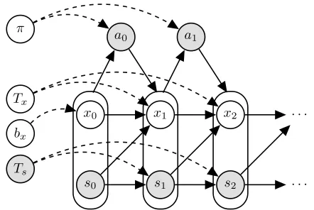
Figure 1: AMM, a model of sequential decision-making be-havior. Each node represents a random variable, and the ob-served variables are shown in grey. Decision factorssandx
(included in the oval supernode) impact the decision choices
a, based on the policyπ(a|s, x). The parametersTxandTs specify the probability for the next state given the previous state and the action, andbxmodels the initial probability.
both the number of goals,|X|, and their dynamics (the way in which the next goal is chosen),Tx, are unknown. While both(x, s)impact the agent’s choice of action (the direction in which the agent moves), the next position depends only on the current position and the action. Thus, the transition probabilities exhibit the factored structure of Eq. 1.
Related Models The AMM shares properties with exist-ing models for sequential decision-makexist-ing. However, it also includes specific features for incorporating domain knowl-edge and facilitating model alignment. Recently, Panella and Gmytrasiewicz used probabilistic deterministic finite state controllers (PDFCs) to model the behavior of another agent. A PDFC models the state transition as deterministic, and thus can be derived as a special case of the AMM with deter-ministicTf. Further, in contrast with the PDFC, the AMM uses a factored representation for the state variable, which allows the model to incorporate known dynamics of the state (via Ts), and prior knowledge regarding the impact of the known state on the agent’s policy (via priors forπ).
Inclusion of a reward function R within the AMM de-scribes an agent executing policy π in a factored Markov decision process (MDP) given by the tuple (F, A, Tf, R) (Puterman 2014). Since agents may not behave rationally (Kahneman 2003), by directly representing π to describe decision-making, the AMM does not assume rationality or even goal-oriented behavior on the part of the other agent.
Problem Definition
Consider an agent whose true behavior model is given by the AMM tuple(X, S, A, bx, Tx, Ts, π). An observer seeks to recover this true model, but has partial specification of the agent’s behavior, described as follows:
• partial knowledge of the decision factors,s∈S, • complete knowledge of the agent’s action space,a∈A, • dynamics of the known decision factors,Ts,
• Iexecution traces of the agent’s behavior, where thei-th trace refers to the sequences(si
0:Ni, a
i
0:Ni),
• noisy change point information regarding the latent state – i.e., the indicator variablect =I(xt+1 =xt)which is accurate with probabilitypc, and
• estimates of some elements of the transition function of latent states (i.e., partial knowledge ofTx).
Thus, formally, the problem of learning the decision-making model corresponds to learning the full AMM tuple given the partial tuple(·, S, A,·,·, Ts,·), execution traces, local auxil-iary input (i.e., the change point of latent states), and global auxiliary input (i.e., partial knowledge ofTx). In this section, we elaborate upon various inputs for the learning problem.
Known AMM Parameters and Execution Traces In the grid-based example introduced above, we have already dis-cussed the specification of the known statess∈Sand actions
a∈A. The specification ofTscorresponds to the known dy-namics of the agent motion and the map of the grid world. The factored representation of AMM allows us to directly incorporate this partial specification(S, A, Ts)of the agent’s model. Execution traces, then, correspond to the sequences of the agent’s position and action, both of which are readily observable within this domain. The problem of learning the model via execution traces and the partial AMM tuple bears similarity to the classical IRL setting; however, in the current problem, the execution trace includes only the partial state. While approaches exist for IRL in partially observable en-vironments, these methods assume knowledge about the set of latent variables and their dynamics (Bogert et al. 2016; Choi and Kim 2011). However, this knowledge, namelyX
andTx, is absent while learning the AMM.
Auxiliary Input While decision factors may not be com-pletely known, partial specifications are often available. This information can be provided by human experts, other algo-rithms or directly from the decision-maker, e.g., (Chernova and Thomaz 2014; Johnson and Willsky 2013). For human-agent interaction, ensuring that the learned model conforms to this information is critical for maintaining model align-ment. In the grid-world example, the number of goals,|X|, and their dynamics,Tx, are unknown to the observer; how-ever, domain knowledge in the form of regions where no goal exists may be available. Such information constraints the dynamics of the latent state and partially specifies the transition functionTx. Furthermore, the goal is but one ex-ample of the latent state; in other applications, the latent state may correspond to other difficult-to-quantify variables, such
as workload and attention. For such variables, constraints re-garding their dynamics can be obtained based on cognitive theories and models (Proctor and Van Zandt 2018).
We refer to the partial specification ofTx as the global auxiliary input, since it applies to all execution traces of the agent. In addition, local information may be queried from a domain expert or the decision maker regarding a specific execution trace. For instance, in the grid-world example, for a given execution trace, an expert can provide estimates of when the agent changed its goal. This corresponds to the change point information regarding the latent state ct, and is referred to as the local auxiliary input. To account for the fact that the expert can make errors, we model the input as accurate with a probabilitypc. We emphasize that while both auxiliary inputs are related to the latent state, they focus on the change in the latent state and do not assume knowledge of the specific label (value) of the latent state. In our prob-lem,xcorresponds to an unknown variable, thus, obtaining labels of this variable from human experts is not possible.
Bayesian AMM Learning
We adopt a Bayesian approach to recover the AMM param-eters given the partial AMM tuple and data (execution traces and auxiliary input). We view the unknown model parame-ters and state sequences as latent random variables, and seek to infer their posterior using the data. In this paper, we limit our scope to those AMMs in whichxis a scalar.
Prior Distributions The AMM tuple provides a genera-tive model for an agent’s behavior; however, since the tuple is only partially known, we include priors for the unknown AMM parameters in order to compute their posterior. As the set of unknown factors X is unknown a priori, the num-ber of factors x is also unknown. This motivates the use of nonparametric priors for the number of unknown states
nx =|X|, initial distributionbxand transition functionTx. We use hierarchical Dirichlet process (HDP) priors inspired by the infinite HMM model (Teh et al. 2006). Under this HDP prior, the popularity of the latent states is generated via a Dirichlet process (DP). The base distribution over pos-sible latent states, given byβ, can be obtained using a stick-breaking construction with hyper-parameterγ, i.e.,
β(·)∼GEM(γ) (2)
Tx(·|x, s, a)∼DP(α·β), ∀(s, a)andx= 1,2,· · · (3)
The rows of the transition function Tx are also generated using a Dirichlet process (DP) with base distributionβand scaling parameterα. This allows us to share parameters (in this case, the state space of latent states) between the rows of the transition function. The latent states are indexed as positive integers. A similar process is used forbx.
known states. In absence of additional knowledge, a Dirich-let distribution can serve as the policy prior,
π(a|s, x)∼DIR(ρ1:|A|), ∀(s)andx= 1,2,· · · (4)
The graphical model of Fig. 1, along with the priors spec-ified in Eq.2-4, provide a generative model for the AMM. In line with other nonparametric Markov models, we term this model as the infinite AMM (iAMM). The iAMM incor-porates a factorization structure common to several statisti-cal models (cf. Eq. 1 Hoffman et al.), which includes global variables(Tx, bx, π, β), local hidden variables (x0:N), ob-servations(s0:N anda0:N)and hyper-parameters(α, γ, ρ).
Variational Inference with Execution Traces
In general, obtaining the exact posterior distribution of the iAMM is intractable. Hence, we explore approaches that ap-proximate this distribution. Guided by the recent success of stochastic variational inference (SVI) for sequential models with factorization structures similar to the iAMM (Johnson and Willsky 2014), we provide a mean-field variational in-ference algorithm in order to approximate the posterior dis-tribution the iAMM. We first derive the algorithm for the case of execution traces as data, then augment it to incorpo-rate auxiliary input.
In this setting, the data consists of(s, a)traces fromI se-quences:x={xi
0:Ni}
I,s= {si
0:Ni}
I,a= {ai
0:Ni}
I. The
pos-terior distribution of the hidden variables of the iAMM is then denoted asp(x, Tx, bx, π, β|s,a). Mean-field inference approximates this posterior by the product of variational fac-torsq(x)q(Tx)q(bx)q(π)q(β)– i.e., by assuming indepen-dence between the hidden variables. Each variational factor is a distribution with separate parameters. The posterior is obtained as thearg maxof the evidence lower boundL;
L(q)≡Eq
p(x, T
x, bx, π, β|s,a)
q(x)q(Tx)q(bx)q(π)q(β)
(5)
Due to the mean-field assumption, this optimization prob-lem can be solved by iteratively optimizing and up-dating the parameters of the local q(x) and global
q(Tx), q(bx), q(π), q(β)variational factors. Following Hoff-man et al., we use natural gradient ascent for the global vari-ational updates. While the structure of the algorithm is sim-ilar to that of the SVI algorithm for the iHMM (Johnson and Willsky 2014), the variational factors and update equa-tions differ. Here, we include the key terms for inference of the iAMM; for an excellent introduction to variational infer-ence, we refer the reader to (Hoffman et al. 2013).
Local Variational Factor In order to efficiently estimate the latent state sequences in the presence of a nonparametric prior, we utilize the direct assignment truncation (Johnson and Willsky 2014). This requires a truncation parameterK
as input and models the assumption thatK latent states at most are present in the execution traces, i.e.,q(x)=0if any
x > K. The mean-field update for the local variational fac-tors is given as follows:
q(x)∝exp(Eq[lnp(x,data|Tx, bx, π, β, Ts)]) =Qiq(xi)
q(xi)∝exp Eq[lnp(xi0:N, si0:N, ai0:N|Tx, bx, π, β, Ts)] ∝exp Eq[lnp(xi0:N, si0:N, ai0:N|Tx, bx, π, Ts)] =p(xi0:N, si0:N, ai0:N|T˜x,˜bx,π, T˜ s)/Zi (6)
∝exp
ln ˜bx(xi0) +
Ni−1 X
0
ln ˜Tx(xit+1|xit, sit, ait)+
lnTs(sit+1|sit, ati) + ln ˜π(ait|xit, sit)
The tilde denotes the operatorA˜= exp(Eq(A)[lnA])and is
used to provide expectation with respect to the global vari-ational factors. The variable Zi denotes the normalization constant. To compute the normalization constant and given their utility in updating global factors, we compute the for-wardFand backward messagesBfor each sequence.
F(t,j)≡Pr(xt=j, s0:t, a0:t) (7)
=X
k
F(t−1,k)T˜x(j|k, st−1, at−1)
Ts(st|st−1, at−1)˜π(at|j, st)
B(t,j)≡Pr(st+1:N, at+1:N|xt=j, s0:t, a0:t) (8)
=X
k
B(t+1,k)T˜x(k|j, st, at)
Ts(st+1|st, at)˜π(at+1|k, st+1)
F(0,j)= ˜bx(j)˜π(a0|j, s0), B(N,j)= 1, Z =PjF(N,j)
The message computation takesO(N K2)time.
Global Variational Factors The direct assignment trun-cation allows us to represent the base distribution β = (β1:K, βrest), whereβ1:K represents the probability of the firstKstates andβrest≡1−PKk=1βkrepresents the prob-ability of truncated states. For the posterior inference, this results in a Dirichlet prior for the rows ofTxandbxgiven as DIR α·(β1:K, βrest). Due to the conjugacy of the Dirichlet and multinomial distributions, we set the variational factors (approximate posterior) for each row ofTxas follows:
q Tx(·|x=j, s=s, a=a)=DIR(λjsa) (9)
In order to update the global parameters, expected statis-tics are necessary with respect to the local factorq(x). For the transition function this corresponds to the expected tran-sition counts which can be efficiently computed using the forward and backward messages as follows:
ˆ
uTx
kjsa ≡Eq(x)PtI[xt+1=k, xt=j, st=s, at=a] (10) =P
tF(t,j)Ts(s0|s, a) ˜Tx(k|j, s, a)˜π(a0|k, s0)B(t+1,k)/Z
wherea0=a
t+1ands0=st+1. Given the expected transition
counts and conjugacy, the global variational parameters are updated by maximizing the evidence lower bound,
λjsa= arg max
λ L λ;Eq[ηg]=(α·β+ ˆu Tx
·jsa)
(11)
B(λ)represents the multivariate Beta function, andlnB(λ) is the log normalizer of the Dirichlet distribution (cf. Eq. 13 Hoffman et al.). This optimization problem is solved by equating the natural gradient (Amari 1998) of the objective function to zero, resulting in the update:
λjsa←(α·β+ ˆuT·jsax ) (12)
This update in the variational parameterλjsacorresponds to a natural gradient ascent of step size1. For large datasets, stochastic natural gradient ascent can be used by consider-ing only a subset of a dataset when computconsider-ing the expected statistics.
Due to conjugate priors, analysis similar toq(Tx)follows for updatingq(bx) and q(π). However, different expected statistics are required, which are computed as follows:
ˆ
ubx
j ≡Eq(x)I[x0=j] =B0,j/Z (13) ˆ
uπajs≡Eq(x)PtI[at=a, xt=j, st=s] (14) =P
tFt,jBt,jI[at=a, st=s]/Z
To obtain a variational estimate forβ, following (Johnson and Willsky 2014), we compute a point estimateβ∗by min-imizing the evidence lower bound with the constraint that all elements are non-negative.
Variational Inference with Auxiliary Inputs
Priors and hyper-parameters provide one avenue for incor-porating domain knowledge in our Bayesian approach. For instance, knowledge about the policy can be incorporated via the policy priors,ρ. However, the auxiliary inputs can-not be incorporated within the priors, motivating the need for modifications to the model or the inference approach.
Local Input Here, we first discuss how local information regarding change points of the latent states can be incor-porated by augmenting the model. We consider the change point information, when available, as an additional observa-tion with two levels,0and1, and the likelihood functionψ,
ψ(ct=1|xt+1=xt)=pc and ψ(ct=0|xt+16=xt)=pc (15)
pcrepresents the known accuracy of the domain expert. This observation depends on both the current and next states, re-quiring modifications to the local variational factors. The modified message computations and sufficient statistics u
are derived as follows (due to space constraints, we list the function arguments only if they are modified):
q(xi) =p(x0:iN, si0:N, ai0:N, ci0:N|T˜x,˜bx,π, T˜ s, ψ) (16)
F(t,j)≡Pr(xt=j, s0:t, a0:t, c0:t−1) (17)
=P
kF(t−1,k)T˜x(·)Ts(·)˜π(·)ψ(ct−1|k, j)
B(t,j)≡Pr(st+1:N, at+1:N, ct:N−1|xt=j, s0:t, a0:t) (18) =P
kB(t+1,k)T˜x(·)Ts(·)˜π(·)ψ(ct|j, k) ˆ
uTx
kjsa=
P
tF(t,j)Ts(·) ˜Tx(·)˜π(·)B(t+1,k)ψ(ct|j, k)/Z By utilizing the mean-field approximation, given the modi-fied sufficient statistics, no other changes to the global up-date equations are necessary.
Global Input Another available auxiliary input is partial knowledge of the transition function,Tx. For analyzing this global input, without loss of generality, we focus on one row of the transition functionθ ≡Tx(·|j, s, a)with a noisy es-timate of itsk-th element. The auxiliary input corresponds toθk, the estimate for thek-th parameter of the multinomial distributionθ. While the local change point information can be included by augmenting the model, incorporating global auxiliary input as additional observations is not straightfor-ward. Ifθkis modeled as a novel observation ofTx, the ben-efits of conjugacy are lost, necessitating computationally ex-pensive inference schemes. This occurs since the posterior of Tx given this novel observation, despite the mean-field assumption, is no longer a Dirichlet distribution.
In order to utilize the global auxiliary input and still pre-serve the benefits of conjugacy, we utilize a novel approach that incorporates this input as constraints for the variational inference. In this method (briefly), the information aboutθis converted into a set of constraints for the variational param-eters – corresponding to a constraint forλjsa, the variational parameters ofq(Tx(·|x, s, a)). To derive this constraint, we use properties (in the current example, the expected value) of the Dirichlet distribution as follows:
λjsa(k) =θkPiλjsa(i) (19) To compute the posterior, we solve a constrained op-timization problem in which the objective is identical to L and the constraints are derived from the auxiliary input (e.g., Eq. 19). Due to the mean-field assumption, these con-straints apply only to a subset of the global update equa-tions – specifically, to the update of global parameterλjsa given in Eq. 11 – and do not impact the local variational up-dates. Thus, the computationally faster (unconstrained) vari-ational inference can be used for the remaining parameters for which no auxiliary input is available.
We term this inference approach constrained variational inference (CVI). By incorporating auxiliary information as constraints over the variational parameters, the support of the posterior distribution is limited to those regions of vari-ational parameters λthat satisfy the constraints. Thus, our approach functions, in essence, as a weighted prior. We note that CVI provides an approximate posterior by limiting the posterior to be in the same family as the prior, and also that a computationally expensive approach that sacrifices conju-gacy can lead to better estimates. Instead, by utilizing con-strained optimization, our approach emphasizes the benefits of conjugacy – allowing us, in this case, to approximate the posterior ofTxwith the Dirichlet distribution.
Teh et al. provided an inference algorithm for the iHMM, a Bayesian nonparametric (BNP) hidden Markov model for scenarios in which the latent states are unknown (2006). Both sampling and variational inference algorithms for sev-eral extensions of iHMM have since been developed (Fox et al. 2011; Johnson and Willsky 2013; Saeedi et al. 2016). These approaches have been applied to segmentation and clustering of sequential data; however, they do not model agent policy or the decision-making process. Our approach to modeling the unknown state space,X, is inspired by these models and includes the explicit dependence of actions on states in order to model agent decision-making.
BNP extensions of decision-making models, both for planning (Doshi-Velez et al. 2015; Liu, Liao, and Carin 2011) and IRL (Michini and How 2012; Ranchod, Ros-man, and Konidaris 2015; Krishnan et al. 2016), have also been developed. Nonparametric IRL approaches incorporate execution traces as the input data and aim to recover the decision-maker’s latent state dependent reward/policy. They result in better performance than parametric IRL approaches when complete state specification is unavailable, but aim to maximize accrued reward and do not seek to recover the true behavioral model. In contrast, our approach explicitly mod-els the dependence of latent state transitions upon action and known states, and includes mechanisms to ensure alignment of the learned model with the auxiliary information. In order to relax the assumption of rationality, in AMM we directly model policy and do not explicitly represent reward. How-ever, our approach for incorporating partial specifications of agent behavior is general and complementary to prior IRL approaches. In domains that include goal-directed or near-rational behavior, future extensions that combine con-strained variational inference and IRL hold the potential to improve sample complexity.
In their work, Panella and Gmytrasiewicz provided a Bayesian nonparametric approach to learning the PDFC from execution traces. They further used the learned PDFC to define subintentional interactive POMDPs and generate autonomous agent behavior during multi-agent tasks. Our model representation and the associated generative model (iAMM) generalize the PDFC model representation by con-sidering stochastic transition of latent states. Further, in or-der to facilitate model alignment, our approach (a) includes a factored state representation to incorporate available infor-mation regarding the known states(S, Ts, ρs), and (b) pro-vides a mechanism to utilize auxiliary inputs regarding la-tent state sequences and their dynamics.
Recently, approaches that model latent states in sequential behavior using generative adversarial networks (GANs) and conditional variational autoencoders (CVAEs) have been developed (Li, Song, and Ermon 2017; Schmerling et al. 2017). By modeling latent states, these approaches can pdict and generate multimodal behavior. However, they re-quire specification of the number of latent modes and do not model their dynamics. In contrast, by utilizing BNP priors, our approach can jointly learning the number of latent states and their impact upon an agent’s behavior. Another interest-ing direction for future work would be to explore the inte-gration of these techniques with Bayesian nonparametrics.
Experiments
We conducted numerical experiments in order to confirm that the proposed approach can successfully incorporate partial specification of an agent’s behavior. Specifically, through the experiments, we measured the ability of the ap-proach to learn models that are aligned with an agent’s true model. Access to the true model is necessary for measuring model alignment and validating our approach; hence, in the experiments, we utilized two simulated scenarios for which the true model was accurately known.
For each scenario, we first specified the true model as a complete AMM tuple. Using this tuple, we generated the problem inputs (namely, the partial AMM tuple, execution traces, and local and global auxiliary inputs). We also gener-ated a test dataset (a set of execution traces) to compare the predictive performance of the learned model. The problem inputs were then used to learn the missing elements of the AMM tuple and infer the latent state sequences.
Metrics In order to measure the state estimation perfor-mance, we computed the normalized Hamming distance between the inferred and true state sequences using the Munkres algorithm (Saeedi et al. 2016). The Munkres algo-rithm provides a correspondence between the inferred and true state labels, such that the normalized Hamming dis-tance is minimized. We used this correspondence to mea-sure the predictive performance on the test set and the met-rics of model alignment. For measuring model alignment, we utilized a metric inspired by the weighted KL divergence (Panella and Gmytrasiewicz 2017). Specifically, to quantify error in learning the transition probabilitiesTx, we first used the Munkres correspondence to match the rows and columns of the learnedTˆxand trueTx, and computed the KL diver-gence between each matched row. Finally, the metric was obtained as an average score weighted by the relative counts of the input dataηdescribed as follows:
wKL(Tx,Tˆx) =Px,s,aηxsaKL(Tx(·|x, s, a)||Tˆx(·|x, s, a))
Similar procedures were used for measuring error for the parametersπandbx. We also quantified model alignment by computing weighted L2 norm(wL2)in a similar fashion.
Domain Line World Highway
MaxEnt VI VI-L CVI-G CVI-LG MaxEnt VI VI-L CVI-G CVI-LG
Hamming dist. (train) — 0.51 0.39 0.30 0.13 — 0.56 0.36 0.48 0.35
Hamming dist. (test) — 0.53 0.40 0.30 0.14 — 0.63 0.44 0.55 0.42
wKL(Tx,Tˆx) — 2.01 1.38 0.98 0.43 — 2.11 1.12 1.03 0.64
wKL(π,ˆπ) 1.08 0.77 0.56 0.41 0.19 1.04 0.48 0.38 0.38 0.33
wKL(bx,ˆbx) — 0.85 0.87 0.53 0.51 — 1.67 1.75 1.50 1.58
Table 1: State inference and model alignment errors. The results are averaged over twenty-five trials for each domain. For both MaxEnt and VI, the input was agent’s execution traces. Auxiliary inputs – either local (L), global (G) or both (LG) – were provided as additional inputs to the other approaches. All algorithms but MaxEnt model unknown states by utilizing AMM as the underlying model. Metrics for state estimation (Hamming dist.) and alignment ofTxandbxare undefined for MaxEnt.
The remaining versions demonstrated the utility of our ap-proach for different input settings. Identical priors, hyper-parameters, initialization and termination conditions were used for all the algorithms.
The four versions of our algorithm all perform inference using the AMM model and thus learn the impact of unknown states. In order to evaluate the effect of modeling unknown states (x), we further compared the performance of our al-gorithms with a representative approach that does not model unknown states, namely, Maximum Entropy IRL (MaxEnt) (Ziebart et al. 2008). Inference of unknown states is not possible using MaxEnt and the metrics Hamming distance,
wKL(Tx,Tˆx)andwKL(bx,ˆbx)are undefined. However, the policy alignment can be quantified using the weighted KL divergence between the true and learned policies.
For each domain, we compared the performance of the algorithms across twenty-five simulation trials. We imple-mented our algorithms as an extension ofpyhsmm, a Python library for approximate unsupervised inference. For CVI, a constrained optimizer is required to solve the resulting constrained optimization problem; towards this end, we uti-lized SLSQP, a sequential least squares programming opti-mization algorithm as implemented inscipy(Kraft 1994; Jones et al. 2001).
Line World
The grid world example described earlier was used as the first evaluation scenario. An agent navigating a one-dimensional grid of length five was considered, with its goal as the latent statexand position as the known states. The action space of the agent included three actions: left, right and wait. The known transition dynamicsTswere modeled as deterministic. The set of agent goalsX included either ends of the grid. The agent exhibited goal-directed motion, and switched its goal after reaching the current goal.
The inputs to the learning algorithm included the partial AMM tuple(S, A, Ts), five execution traces (each of length 20), and the auxiliary inputs. Noisy change point informa-tion for two execuinforma-tion traces with accuracypc=0.9served as the local input. The region of the grid where the agent did not switch its goal was randomly selected and specified as the global input. Additionally, five execution traces were gener-ated as the test set. The objective of the learning algorithm
was to recover the set of goalsX, their switching dynamics
Txand the agent’s policyπ. Despite the small domain size, the learning problem was challenging since different model parameters (Tx, π) could generate identical behavior. Fur-ther, depending on its goal the agent chose different actions for the same location, and execution traces included cycles.
The results of the experiments, averaged over the twenty-five trials, are summarized in Table 1. We observed that our complete approach CVI-LG resulted in models with better alignment (lowerwKL scores) as compared to the remain-ing baselines. Similar trends were observed for the model alignment metrics computed using the weighted L2 norm. Along with improved model alignment, CVI-LG resulted in lower Hamming distance between the true and inferred se-quences for both the training and test datasets. Utilization of only one auxiliary input also improved upon the base-line VI that relies only on execution traces. This validates that our approach is capable of utilizing auxiliary informa-tion when available. Interestingly, while the auxiliary inputs did not include information regarding the agent’s policy, the alignment between the true and learned policy improved by incorporating the auxiliary input. This is possible since our approach performs joint inference of the agent’s model pa-rameters (e.g.,Txandπ).
All versions of our algorithm resulted in lower policy alignment error as compared to MaxEnt. Despite identi-cal input data, VI (variational inference applied to AMM) demonstrated better model alignment and could perform state inference. This result indicates the utility of explicitly modeling the unknowns as part of the AMM and learning their impact on the agent’s behavior.
Highway Domain
on the highway, and could choose to switch lanes at each step. The agent’s actions depend on known, observable fac-tors (distance to cars and current lane) as well as latent states (whether it is driving nominally or pursuing a civilian car). The agent switched from nominal driving to pursuing a civil-ian car if two civilcivil-ian cars seemed to be racing (which the agent determined based on the relative distances of the cars), and returned to nominal mode after catching a car. The learn-ing algorithm had access to the known states of the agent, its action space and dynamics of the highway domainTs; how-ever, the number of latent statesx and their dynamicsTx were unknown.
We conducted experiments for the highway domain in a similar fashion to that for the line world scenario; how-ever, longer execution traces (each of length 40) were used for both training and testing datasets. For this domain, the learning algorithm had to reason over a much larger prob-lem with an observable state space of size200. The results of the experiments, averaged over the twenty-five trials, are summarized in Table 1. Similar to the first scenario, the ef-fect of modeling unknowns was evident, as all versions of our approach (including VI) resulted in lower policy align-ment error as compared to MaxEnt. Further, we observed that our approach could successfully incorporate auxiliary inputs and improve model alignment when one or both aux-iliary inputs are available. Lastly, we observed reductions in the state decoding and prediction errors (normalized Ham-ming distance on training and test data, respectively) when the local and global auxiliary inputs were utilized.
Discussions
Through the numerical experiments, we demonstrate that the proposed approach to model learning is capable of learn-ing AMM tuples that are aligned with an agent’s true model and that conform to the partial knowledge of an agent’s be-havior. Furthermore, as more information of varied types (e.g., execution traces, change point sequences, constraints on model parameters) is provided to the inference algorithm, the model alignment improves. This is possible despite in-complete specification of the agent’s decision factors.
The ability to incorporate these novel input types enables the use of high-level information of the agent’s behavior dur-ing the model learndur-ing and specification process. This ap-proach is made possible through the use of a factored model representation and a novel inference algorithm. While prior approaches to learning an agent’s model largely rely on ei-ther execution traces or label/feature queries, we provide an approach that can efficiently utilize different input types (in-cluding input about model parameters) and does not assume complete knowledge of the agent’s feature set (state space).
In our ongoing work, we are exploring interactive exten-sions of the proposed approach, wherein the observer can actively choose to query a human decision-maker (or a do-main expert) regarding additional and potentially informa-tive specifications. The algorithms presented in this work will enable the observer to utilize the queried specifications efficiently. Another application of our approach includes learning models from behavioral data that conform to pref-erences provided, as logical or procedural constraints, by a
human user; the global inputs provide one avenue to incor-porate preferences in our approach.
As mentioned in the introduction, a key motivation behind learning agent models is to enable effective human-machine interaction. The algorithms presented in this work can be used both by a collaborative robot (for learning models of human behavior to improve robot decision-making) and by a human (to learn transparent models of robot behavior to better calibrate trust) (Javdani et al. 2018; Yang et al. 2017). Both of these use cases offer novel research avenues, such as the efficient specification of decision-theoretic models for interaction (such as, POMDPs and decentralized-POMDPs) and evaluation of the utility of aligned models as compared to purely predictive models for human-machine interaction (Oliehoek, Amato, and others 2016).
We identify three areas of further improvement of our ap-proach. Firstly, our approach is limited in that it can learn the latent states and the AMM tuple, but not the semantic labels or interpretation of these latent states. We posit that interaction between a human (domain expert) and the algo-rithm will be necessary for incorporating interpretability in the latent states learned via Bayesian nonparametrics. Sec-ondly, our approach is limited to a scalar latent state and thus utilizes a flat state representation for the latent state. Lastly, we utilize tabular representations for the unknown AMM pa-rameters (namely,π, Tx). We aim in future work to address these limitations through the use of function approximation to represent model variables and factored latent state repre-sentations.
Conclusion
We consider the problem of learning an agent’s true decision-making model with partial specification of its be-havior. To formalize and address this problem, we utilize a factored representation of sequential decision-making be-havior, the agent Markov model (AMM). We pose the learn-ing problem as one of Bayesian inference, and provide novel variational inference algorithms for the AMM that can uti-lize different types of information – including, sequences of observed behavior, prior knowledge of agent’s policy, and partial specification of agent’s state and dynamics. Through numerical experiments, we validate that our approach is capable of utilizing varied information types and, conse-quently, learning models that align with the true behavioral model.
Acknowledgments
We thank Ardavan Saeedi for fruitful discussions on Bayesian inference and learning.
References
Abbeel, P., and Ng, A. Y. 2004. Apprenticeship Learning via Inverse Reinforcement Learning. InIntl. Conf. on Machine Learning (ICML). ACM.
Amari, S.-I. 1998. Natural Gradient Works Efficiently in Learning.Neural Computation10(2):251–276.
Bogert, K.; Lin, J. F.-S.; Doshi, P.; and Kulic, D. 2016. Expectation-Maximization for Inverse Reinforcement Learning with Hidden Data. InIntl. Conf. on Autonomous Agents and Multi-Agent Systems (AAMAS), 1034–1042. Chernova, S., and Thomaz, A. L. 2014. Robot Learning from Human Teachers. Synthesis Lectures on Artificial In-telligence and Machine Learning8(3):1–121.
Choi, J., and Kim, K.-E. 2011. Inverse Reinforcement Learning in Partially Observable Environments. Journal of Machine Learning Research12(Mar):691–730.
Doshi-Velez, F.; Pfau, D.; Wood, F.; and Roy, N. 2015. Bayesian Nonparametric Methods for Partially-Observable Reinforcement Learning. IEEE Trans. on Pattern Analysis and Machine Intelligence37(2):394–407.
Fox, E. B.; Sudderth, E. B.; Jordan, M. I.; and Willsky, A. S. 2011. A Sticky HDP-HMM with application to Speaker Di-arization.The Annals of Applied Statistics1020–1056. Fridman, L.; Reimer, B.; Mehler, B.; and Freeman, W. T. 2018. Cognitive Load Estimation in the Wild. InCHI Conf. on Human Factors in Computing Systems, 652. ACM. Hoffman, M. D.; Blei, D. M.; Wang, C.; and Paisley, J. 2013. Stochastic Variational Inference.Journal of Machine Learn-ing Research14(1):1303–1347.
Javdani, S.; Admoni, H.; Pellegrinelli, S.; Srinivasa, S. S.; and Bagnell, J. A. 2018. Shared Autonomy via Hindsight Optimization for Teleoperation and Teaming. The Interna-tional Journal of Robotics Research.
Johnson, M. J., and Willsky, A. S. 2013. Bayesian Nonpara-metric Hidden Semi-Markov Models. Journal of Machine Learning Research14(Feb):673–701.
Johnson, M., and Willsky, A. 2014. Stochastic Variational Inference for Bayesian Time Series Models. InIntl. Conf. on Machine Learning, 1854–1862.
Jones, E.; Oliphant, T.; Peterson, P.; et al. 2001. SciPy: Open Source Scientific Tools for Python.
Jonker, C. M.; Van Riemsdijk, M. B.; and Vermeulen, B. 2011. Shared Mental Models: A Conceptual Analysis. InCoordination, Organizations, Institutions, and Norms in Agent Systems (COIN). Springer. 132–151.
Kahneman, D. 2003. Maps of Bounded Rationality. The American Economic Review93(5):1449–1475.
Kraft, D. 1994. Algorithm 733: TOMP–Fortran modules for Optimal Control Calculations.ACM Trans. on Mathematical Software (TOMS)20(3):262–281.
Krishnan, S.; Garg, A.; Goldberg, K.; et al. 2016. SWIRL: A Sequential Windowed Inverse Reinforcement Learning Al-gorithm for Robot Tasks with Delayed Rewards. In Work-shop on the Algorithmic Foundations of Robotics (WAFR). Kumar, P., and Varaiya, P. 2016.Stochastic Systems. SIAM. Li, Y.; Song, J.; and Ermon, S. 2017. InfoGAIL: Inter-pretable Imitation Learning from Visual Demonstrations. In
Advances in Neural Information Processing Systems (NIPS), 3812–3822.
Liu, M.; Liao, X.; and Carin, L. 2011. The Infinite Re-gionalized Policy Representation. InIntl. Conf. on Machine Learning (ICML). ACM.
Majumdar, A.; Singh, S.; Mandlekar, A.; and Pavone, M. 2017. Risk-Sensitive Inverse Reinforcement Learning via Coherent Risk Models. InRobotics: Science and Systems. Michini, B., and How, J. 2012. Bayesian Nonparametric In-verse Reinforcement Learning. InJoint European Conf. on Machine Learning and Knowledge Discovery in Databases. Springer.
Oliehoek, F. A.; Amato, C.; et al. 2016.A Concise Introduc-tion to Decentralized POMDPs, volume 1. Springer. Panella, A., and Gmytrasiewicz, P. 2017. Interactive POMDPs with Finite-State Models of Other Agents. Au-tonomous Agents and Multi-Agent Systems31(4):861–904. Proctor, R. W., and Van Zandt, T. 2018. Human Factors in Simple and Complex Systems. CRC Press.
Puterman, M. L. 2014. Markov Decision Processes: Dis-crete Stochastic Dynamic Programming. Wiley & Sons. Ramachandran, D., and Amir, E. 2007. Bayesian Inverse Reinforcement Learning. InIntl. Joint Conf. on Artificial Intelligence (IJCAI).
Ranchod, P.; Rosman, B.; and Konidaris, G. 2015. Nonpara-metric Bayesian Reward Segmentation for Skill Discovery using Inverse Reinforcement Learning. InIntl. Conf. on In-telligent Robots and Systems (IROS), 471–477. IEEE. Sadigh, D.; Sastry, S.; Seshia, S. A.; and Dragan, A. D. 2016. Planning for Autonomous Cars that Leverages Effects on Human Actions. InRobotics: Science and Systems (R:SS). Saeedi, A.; Hoffman, M.; Johnson, M.; and Adams, R. 2016. The Segmented iHMM: a Simple, Efficient Hierarchical In-finite HMM. InIntl. Conf. on Machine Learning (ICML). Schmerling, E.; Leung, K.; Vollprecht, W.; and Pavone, M. 2017. Multimodal Probabilistic Model-Based Planning for Human-Robot Interaction.arXiv preprint.
Teh, Y. W.; Jordan, M. I.; Beal, M. J.; and Blei, D. M. 2006. Hierarchical Dirichlet Processes. Journal of the American Statistical Association101(476):1566–1581.
Thomaz, A.; Hoffman, G.; Cakmak, M.; et al. 2016. Compu-tational Human-Robot Interaction. Foundations and Trends in Robotics4(2-3):105–223.
Unhelkar, V. V., and Shah, J. A. 2018. Learning Models of Sequential Decision-Making without Complete State Speci-fication using Bayesian Nonparametric Inference and Active Querying. Technical report, Massachusetts Institute of Tech-nology (MIT).
Yang, X. J.; Unhelkar, V. V.; Li, K.; and Shah, J. A. 2017. Evaluating Effects of User Experience and System Trans-parency on Trust in Automation. InIntl. Conf. on Human-Robot Interaction (HRI), 408–416. ACM.