R E S E A R C H
Open Access
Latent class model with application to
speaker diarization
Liang He
1*, Xianhong Chen
1, Can Xu
1, Yi Liu
1, Jia Liu
1and Michael T. Johnson
2Abstract
In this paper, we apply a latent class model (LCM) to the task of speaker diarization. LCM is similar to Patrick Kenny’s variational Bayes (VB) method in that it uses soft information and avoids premature hard decisions in its iterations. In contrast to the VB method, which is based on a generative model, LCM provides a framework allowing both generative and discriminative models. The discriminative property is realized through the use of i-vector (Ivec), probabilistic linear discriminative analysis (PLDA), and a support vector machine (SVM) in this work. Systems denoted as LCM-Ivec-PLDA, LCM-Ivec-SVM, and LCM-Ivec-Hybrid are introduced. In addition, three further improvements are applied to enhance its performance. (1) Adding neighbor windows to extract more speaker information for each short segment. (2) Using a hidden Markov model to avoid frequent speaker change points. (3) Using an agglomerative hierarchical cluster to do initialization and present hard and soft priors, in order to overcome the problem of initial sensitivity. Experiments on the National Institute of Standards and Technology Rich Transcription 2009 speaker diarization database, under the condition of a single distant microphone, show that the diarization error rate (DER) of the proposed methods has substantial relative improvements compared with mainstream systems. Compared to the VB method, the relative improvements of LCM-Ivec-PLDA, LCM-Ivec-SVM, and LCM-Ivec-Hybrid systems are 23.5%, 27.1%, and 43.0%, respectively. Experiments on our collected database, CALLHOME97, CALLHOME00, and SRE08 short2-summed trial conditions also show that the proposed LCM-Ivec-Hybrid system has the best overall performance.
Keywords: Speaker diarization, Variational Bayes, Latent class model, i-vector
1 Introduction
Speaker diarization task aims to address the problem of “who spoke when” in an audio stream by splitting the audio into homogeneous regions labeled with speaker identities [1]. It has a wide application in automatic audio indexing, document retrieving and speaker-dependent automatic speech recognition.
In the field of speaker diarization, variational Bayes (VB) proposed by Patrick Kenny [2–5] and VB-hidden Markov model (HMM) introduced by Mireia Diez [6] have become the state-of-the-art approaches. This system has two characteristics. First, unlike mainstream approaches (i.e., segmentation and clustering approaches, discussed in the following section), it uses a fixed-length segmentation instead of speaker change point detection to do speaker segmentation, dividing an audio recording into uniform
*Correspondence:[email protected]
1Department of Electronic Engineering, Tsinghua University, Zhongguancun Street, 100084 Beijing, China
Full list of author information is available at the end of the article
and short segments. These segments are short enough that they can be regarded as each containing only one speaker. This type of segmentation leaves the difficulty to the clustering stage and requires a better clustering algo-rithm that includes temporal correlation. Second, the VB approach utilizes a soft clustering approach that avoids premature hard decisions. Despite its accuracy, there are still some deficiencies of the approach. The VB approach is a single-objective method. Its goal is to increase the overall likelihood, which is based on a generative model, not to distinguish speakers. Furthermore, because the seg-mented segments are very short, the probability that an individual segment occurs given a particular speaker is inaccurate and may degrade system performance. In addi-tion, some researchers have also noted that the VB system is very sensitive to its initialization conditions [7]. For example, if one speaker dominates the recording, a ran-dom prior tends to result in assigning the segments to each speaker evenly, leading to a poor result.
In this paper, to address the drawbacks of VB, we apply a latent class model (LCM) to speaker diarization. LCM was initially introduced by Lazarsfeld and Henry [8]. It is usually used as a way of formulating latent attitu-dinal variables from dichotomous survey items [9, 10]. This model allows us to compute p(Xm,Ys,ims), which represents the likelihood that both the segment repre-sentationXm and the estimated class representationYs are from the same speaker, in a more flexible and criminative way. We introduce the probabilistic linear dis-criminative analysis (PLDA) and support vector machine (SVM) into the computation, and propose LCM-Ivec-PLDA, LCM-Ivec-SVM, and LCM-Ivec-Hybrid systems. Furthermore, to address the problem caused by the short-ness of each segment, in consideration of speaker tem-poral relevance, we take Xm’s neighbors into account at the data and score levels to improve the accuracy of p(Xm,Ys). A hidden Markov model (HMM) is applied to smooth frequent speaker changes. When the speakers are imbalanced, we use an agglomerative hierarchical cluster (AHC) approach [11] to address the system sensitivity to initialization.
The parameter selection experiments are mainly car-ried out on the NIST RT09 SPKD database [12] and our collected speaker imbalanced database. In practice, the number of speakers in a meeting or telephone call is relatively easy to be obtained. We assume that this number is known in advance. RT09 has two evaluation conditions: single distant microphone (SDM), where only one microphone channel is involved; and multiple distant microphone (MDM), where multiple microphone chan-nels are involved. In this paper, we mainly consider the speaker diarization task under the SDM condition. We also conduct performance comparison experiments on the RT09, CALLHOME97 [13], CALLHOME00 (a sub-task of NIST SRE00), and SRE08 short2-summed trial condition. Experiment results show that the proposed method has better performance compared with the main-stream systems.
The remainder of this paper is organized as follows. Section 2 describes mainstream approaches and algo-rithms. Section3introduces the latent class model (LCM), and Section 4 realizes the PLDA, LCM-Ivec-SVM, and LCM-Ivec-Hybrid systems. Further improve-ments are presented in Section5. Section6discusses the difference between our proposed methods and related works. Experiments are carried out and the results are analyzed in Section7. Conclusions are drawn in Section8.
2 Mainstream approaches and algorithms
Speaker diarization is defined as the task of labeling speech with the corresponding speaker. The most com-mon approach consists of speaker segmentation and clustering [1,14].
The mainstream approach to speaker segmentation is finding speaker change points based on a similarity met-ric. This includes Bayesian information criterion (BIC) [15], Kullback-Leibler [16], generalized likelihood ratio (GLR) [17], and i-vector/PLDA [18]. More recently, there are also some metrics based on deep neural networks (DNN) [19, 20], convolutional neural networks (CNN) [21,22], and recurrent neural networks (RNN) [23,24]. However, the DNN-related methods need a large amount of labeled data and might suffer from a lack of robustness when working in different acoustic environments.
In speaker clustering, the segments belonging to the same speaker are grouped into a cluster. The problem of measuring segment similarity remains the same as for speaker segmentation and the metrics described above can also be used for clustering. Cluster strategies based on hard decisions include agglomerative hierarchical cluster-ing (AHC) [11] and division hierarchical clustering (DHC) [25]. A soft decision-based strategy is the variational Bayes (VB) [5], which is combined with eigenvoice modeling [2]. Taking temporal dependency into account, HMM [6] and hidden distortion models (HDM) [26,27] are successfully applied in speaker diarization. There are also some DNN-based clustering strategies. In [28], a clustering algorithm is introduced by training a speaker separation DNN and adapting the last layer to specific segments. Another paper [29] introduces a DNN-HMM-based clustering method, which uses a discriminative model rather than a gener-ative model, i.e., replacing GMMs with DNNs, for the estimation of emission probability, achieving better per-formance.
Some diarization systems based on i-vector, VB, or DNN are trained in advance, rely on the knowledge of application scenarios, and require large amount of matched training data. They perform well in fixed con-ditions. While some other diarization systems, such as BIC, HMM, or HDM, have little prior training. They are condition independent and more robust to the change of conditions. They perform better if the conditions, such as channels, noises, or languages, vary frequently.
2.1 Bottom-up approach
cosine distance [33] or probabilistic linear discriminant analysis (PLDA) [34–37] is usually used. The stopping cri-teria can be based on thresholds, or on a pre-assumed number of speakers, alternatively [38,39].
Bottom-up approach is more sensitive to nuisance vari-ations (compared with the top-down approach), such as speech channel, speech content, or noise [40]. A similar-ity function, which is robust to these nuisance variations, is crucial to this approach.
2.2 Top-down approach
The top-down approach is usually referred to as a divisive hierarchical clustering (DHC) [25]. In contrast with the bottom-up approach, the top-down approach first treats all segments as unlabeled. Based on a selection criterion, some segments are chosen from these unlabeled seg-ments. The selected segments are attributed to a new clus-ter and labeled. This selection procedure is repeated until no more unlabeled segments are left or until the stop-ping criteria, similar to those employed in the bottom-up approach, is reached. The top-down approach is reported to give worse performance on the NIST RT database [25] and has thus received less attention. However, paper [40] makes a thorough comparative study of these two approaches and demonstrates that these two approaches have similar performance.
The top-down approach is characterized by its high-computational efficiency but is less discriminative than the bottom-up approach. In addition, top-down is not as sensitive to nuisance variation and can be improved through cluster purification [25].
Both approaches have common pitfalls. They make premature hard decisions which may cause error prop-agation. Although these errors can be fixed by Viterbi resegmentation in next iterations [40,41], a soft decision is still more desirable.
2.3 Hidden distortion model
Different from AHC or DHC, HMM takes temporal dependencies between samples into account. Hidden dis-tortion model (HDM) [26,27] can be seen as a generaliza-tion of HMM to overcome its limitageneraliza-tions. HMM is based on the probabilistic paradigm while HDM is based on the distortion theory. In HMM, there is no regularization option to adjust the transition probabilities. In HDM, a regularization of transition cost matrix, used as a replace-ment of transition probability matrix, is a natural part of the model. Both HMM and HDM do not suffer from error propagation. They do re-segmentation via a Viterbi or forward-backward algorithm. And each iteration may fix errors in previous loops.
2.4 Variational Bayes
Variational Bayes (VB) is a soft speaker clustering method
introduced to address speaker diarization task [2, 5, 6]. Suppose a recording is uniformly segmented into fixed-length segmentsX = {X1,· · ·,Xm,· · ·,XM}, where the subscript m is the time index, 1 ≤ m ≤ M. M is the segment duration. LetY = {Y1,· · ·,Ys,· · ·,YS}be the speaker representation, wheresis the speaker index, 1≤ s≤S.Sis the speaker number.I= {ims}, whereims repre-sents whether a segmentmbelongs to a speakersor not. In speaker diarization,X is the observable data,Y andI are the hidden variables. The goal is to find properYandI to maximize logq(X). According to the Kullback-Leibler divergence, the lower bound of the log likelihood logq(X) can be expressed as
logq(X)≥
q(Y,I)lnq(X,Y,I) q(Y,I) dYdI
The equality holds if and only ifq(Y,I) = q(Y,I|X). The VB assumes a factorizationq(Y,I) = q(Y)q(I) to approximate the true posteriorq(Y,I|X)[2]. Then,q(Y) andq(I)are iteratively refined to increase the lower bound of logq(X). The final speaker diarization label can be assigned according to segment posteriors [2]. The imple-mentation of VB approach is shown in Algorithm 1. Compared with the bottom-up or top-down approach, the VB approach uses a soft decision strategy and avoids a premature hard decision.
Algorithm 1:Variational Bayes
1: Voice activity detection and feature extraction 2: Speaker segmentation
2.1: Split an audio intoMshort fixed-length segments.
3: Clustering 3.1:
For each speaker s, calculate speaker dependent Baum-Welch statistics and update speaker model
Ys. 3.2:
For each segment m and speakers, compute and update segment posteriors via eigenvoice scoring.
3.3: Viterbi or forward-backward realignment with minimum duration constraint.
3.4 Repeat 3.1–3.3 until stopping criteria is met.
3 Latent class model
Suppose a sequenceX is divided intoMsegments, and
This relationship is denoted by the latent class indicator matrixI= {ims}
ims=
1, if segmentmbelongs to the latent classs 0, if segmentmdoes not belong to the latent classs
(1)
Our objective function is to maximizes the log-likelihood function with constraint that there areSclasses, as follows
argQ,Ymax logp(X,Y,I)=argQ,Ymax M
m=1 log
S
s=1 p(Xm,Ys,ims)
s.t S classes
(2)
whereQ = {qms},qms is the posterior probability which will be explained later. Intuitively, if p(Xm,Ys,ims) > p(Xm,Ys,ims),s=s, 1≤s,s≤S, we will draw a conclu-sion that segmentmbelongs to classs. The above formula is intractable for the unknownYandI. We solve it through an iterative algorithm by introducingQas follows:
1 The objective function is factorized as
M
m=1 log
S
s=1
p(Xm,Ys,ims)= M
m=1 log
S
s=1
p(Xm,Ys)p(ims|Xm,Ys)
=
M
m=1 log
S
s=1
p(Xm,Ys)qms
(3)
In this step,p(Xm,Ys)is assumed to be known. We useqmsdenotep(ims|Xm,Ys)for simplicity. Note that,qms ≥0andSs=1qms=1. The (3) is optimized by Jensen’s inequality and Lagrange multiplier method. The updatedq(msu)is
q(msu)= Sqmsp(Xm,Ys) s=1qmsp(Xm,Ys)
(4)
The explanation for step 1 is thatqmsis updated, givenp(Xm,Ys)is known.
2 The objective function is factorized as
M
m=1 log
S
s=1
p(Xm,Ys,ims)= M
m=1 log
S
s=1
p(ims)p(Xm,Ys|ims)
≈
M
m=1 log
S
s=1
qmsp(Ys)p(Xm|Ys,ims)
(5)
There are two approximations used in this step. First, we use the posterior probabilityqmsin step 1 as the prior probabilityp(ims)in this step. Second, p(Ys|ims)=p(Ys)is assumed. According to our understanding,Ysis the speaker representation and imsis the indicator between segment and speaker. SinceXmis not referenced,Ysandimsare assumed to
be independent of each other. A similar explanation is also given in Kenny’s work, see (10) in [2]. The goal of this factorization is to putYson the position of parameter, which provides a way to optimize it. And this step is to estimateYs, givenp(ims)is known. 3 The objective function is factorized as
M
m=1 log
S
s=1
p(Xm,Ys,ims)= M
m=1 log
S
s=1
p(ims)p(Xm,Ys|ims)
≈
M
m=1 log
S
s=1
qmsp(Xm)p(Ys|Xm,ims)
(6)
There are also two approximations used in this step. First, we use the posterior probabilityqmsin step 1 as the prior probabilityp(ims)in this step. Second, p(Xm|ims)=p(Xm)is assumed. According to our understanding,Xmis the segment representation andimsis the indicator between segmentm and speakers. SinceYsis not referenced,Xmandimsare assumed to be independent of each other. The explanation for step 3 is thatp(Xm,Ys|ims)is calculated, givenp(ims)andYsare known. We compute the posterior probabilityp(Ys|Xm,ims) rather thanp(Xm|Ys,ims)to approximate
p(Xm,Ys|ims)with the goal that this factorization is to take advantages ofS speaker constraint. In next loop,p(Xm,Ys|ims)is used as the approximation of p(Xm,Ys)and go to step 1, see Fig.1.
After a few iteration, theqmsis used to make the final binary decision. We have several comments on the above iterations
• Although the form of objective function
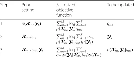
(argQ,Ymax logp(X,Y,I)) is the same in these three steps, the prior setting, factorized objective function and variables to be optimized are different, see Table1and Fig.1. This will also be further verified in the next section.
• The connection between step 1 and steps 2 and 3 are p(ims)andp(Xm,Ys), see the upper left text box in Fig.1. We use the posterior probability
(p(ims|Xm,Ys)andp(Xm,Ys|ims)) in the previous step or loop as the prior probability (p(ims)and p(Xm,Ys)) in the current step or loop.
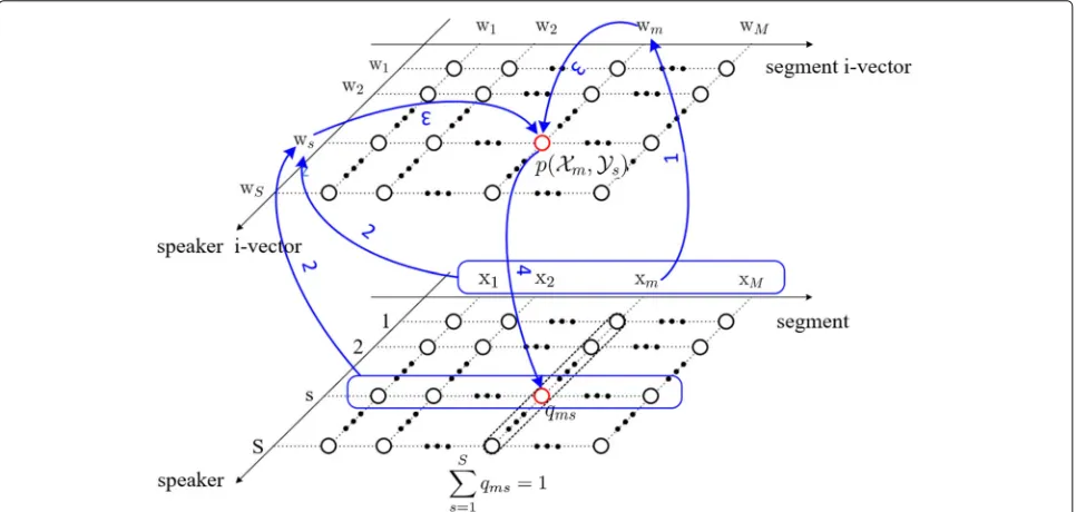
Fig. 1Diagram of LCM. The upper left text box illustrates the relationship between step 1 and steps 2 and 3. The lower left text box explains the difference between step 2 and step 3
• A unified objective function or not? Not necessary. Of course, a unified objective function is more rigorous in theory, e.g., VB [2]. In fact, we can use the above model to explain the VB in [2]. The (15), (19), and (14) in [2] are corresponding to steps 1, 2, and 3, respectively1. However, the prior setting in each step is different, as stated in Table1, we can take advantage of it to make a better estimation or computation. For example, we have two additional ways to improve p(Ys,Xm|ims)in step 3, compared with the VB. First, the (14) in [2] is the eigenvoice scoring, givenXmand
Ysare known, which can be further improved by more effective scoring method, e.g., PLDA. Second, there areS classes constraint, turning the open-set problem into the close-set problem.
• Whether the loop is converged? Not guaranteed. Since the estimation ofYsand computation of p(Xm,Ys|ims)are choices of designers, the loop will not converge for some poor implementation. But, if pu(Xm,Ysu∗|ims∗=1) >p(Xm,Ys∗|ims∗=1) (monotonically increase with upper bound) is satisfied, the loop will converge to a local or global optimal. The notation with star means that it’s the ground truth. TheYwith a superscriptu means the updatedYin step 2 and thep with a superscript u means another (or updated) similarity function in step 3. This also implies that we have two ways to
optimize the objective function. One is to use a better
Y(e.g., updatedYin step 2) and the other one is to choose a more effective similarity function. • Whether the converged results conform to the
diarization task? The Kullback-Leibler divergence betweenQ and I isDKL(IQ)= −Mm=1logqms. The minimization of KL divergence betweenQ and I is equal to the maximization ofMm=1logqms. According to (3),qmsdepends onp(Xm,Ys). If p(Xm,Ys∗) >p(Xm,Ys),s∗=s(ims∗=1is the ground truth), the converged results will satisfy the diarization task.
• In addition to explicit unknownQ andY, the unknown factors also include implicit functions, e.g., p(Xm,Ys|ims)in steps 2 and 3. These implicit
Table 1Settings for LCM in each step
Step Prior
setting
Factorized objective function
To be updated
1 p(Xm,Ys) Mm=1log
S s=1 p(Xm,Ys)qms
qms
2 Xm,qms Mm=1log
S s=1qms
p(Xm|Ys,ims)p(Ys)
Ys
3 Xm,qms,Ys Mm=1log
S s=1 qmsp(Ys|Xm,ims)p(Xm)
functions are statistical models selected by designers in implementation. What we want to emphasize is that we can do optimization on its parameters for a already selected function, we can also do
optimization by choosing more effective functions based on known setting, e.g., from eigenvoice to PLDA or SVM scoring.
4 Implementation
If we regard speakers as latent classes, LCM will be a natural solution to a speaker diariazation task. The implementation needs to solve three things further: specify the segment representationXm, specify the class representationYsand p(Xm,Ys)computation. Depending on different consider-ations, they can incorporate different algorithms. Given VB, LCM-Ivec-PLDA, and LCM-Ivec-SVM as examples,
1 In VB,Xmis an acoustic feature.Ysis specified as a speaker i-vector.p(Xm,Ys)is the eigenvoice scoring (Eq. (14) in [2]).
2 In LCM-Ivec-PLDA,Xmis specified as a segment i-vector.Ysis specified as a speaker i-vector. p(Xm,Ys)is calculated by PLDA.
3 In LCM-Ivec-SVM,Xmis specified as a segment i-vector.Ysis specified as a SVM model trained on speaker i-vectors.p(Xm,Ys)is calculated by SVM .
Actually,p(Xm,Ys)can be regarded as a speaker verifi-cation task of short utterances, which will benefit from the large number of previous studies on speaker verification.
The implementation of presented LCM-Ivec-PLDA speaker diarization is shown in Fig. 2. Different from the above section,X andY are abstract representations of segment m and speaker s. In this section, they are specified to explicit expressions. To avoid confusion, we use x, X, and w to denote an acoustic feature vector, an acoustic feature matrix and an i-vector. After front-end processing, the acoustic feature X of a whole recording is evenly divided into M segments, X = {x1,· · ·, xM}. Based on the above notations, the iterative procedures of LCM-Ivec-PLDA is as follows (Fig.2):
1 segment i-vectorwmis extracted fromxmand its neighbors, which will be further explained in Section5.
2 speaker i-vectorwsis estimated based onQ= {qms} andX= {xm}.
3 p(Xm,Ys)=p(wm, ws)is computed through PLDA scoring.
4 Updateqmsbyp(Xm,Ys).
This above process is repeated until the stopping crite-rion is met. The step 1 is a standard i-vector extraction procedure [42] and step 4 is realized by (4). So, we will put more attention on steps 2 and 3 in the following subsections.
4.1 Estimate speaker i-vector ws
If T denotes the total variability space, our objective function [2] is as follows
Fig. 2Diagram of LCM speaker diarization. Step 1: extract segment i-vector wm. Step 2: extract speaker i-vector ws. Step 3: computep(Xm,Ys). Step
argYsmax M
m=1 log
S
s=1
qmsp(Xm,Ys)
=argwsmax M
m=1 log
S
s=1
qmsp(xm|ws)p(ws)
=argwsmax M
m=1 log
S
s=1 qms
C
c=1
ωcN(xm|μubm,c+Tcws,ubm,c)
N(ws|0,IR)
(7)
where C is the number of Gaussian mixture compo-nents.N is a Gaussian distribution.ωc,μubm,c, andubm,c are the weight, mean vector, and covariance matrix of the cth component of UBM, respectively.IR is an iden-tity matrix with rankR. In contrast to speaker recognition in which the whole audio are assumed to be from one speaker, the segmentmbelongs to speakerswith a prob-ability qms in the case of speaker diarization. We use Jensen’s inequality [43] again and obtain the lower bound as follows
M
m=1 S
s=1 qms
C
c=1
γubm,mclogN(xm|μubm,c+Tcws,ubm,c)
N(ws|0,IR)
(8)
where
γubm,mc= ωcN(
xm|μubm,c,ubm,c) C
c=1ωcN(xm|μubm,c,ubm,c)
(9)
The above objective function is a quadratic optimization problem with the optimal solution
ws=IR+TtNs−1T−1Tt−1Fs (10)
whereNsandFsare concatenations ofNscandFsc, respec-tively. is a diagonal matrix whose diagonal blocks are ubm,m. TheNsc,Fscare defined as follows
Nsc= M
m=1
qmsγubm,mc
Fsc= M
m=1
qmsγubm,mc(xm−μubm,c)
(11)
In the above estimation, T and are assumed to be known. These can be estimated on a large auxiliary database in a traditional i-vector manner.
4.2 Computep(Xm,Ys)
To computep(Xm,Ys), we first extract segment i-vectors wmfrom xmand its neighbors, and evaluate the probabil-ity that wm and ws are from the same speaker. We take
advantages of PLDA and SVM to improve system perfor-mance, and propose LCM-Ivec-PLDA, LCM-Ivec-SVM, and LCM-Ivec-Hybrid systems.
4.2.1 PLDA
As each segment i-vector wmand speaker i-vector wsare known, the task reduces to a short utterance speaker ver-ification task at this stage. We adopt a simplified PLDA [44] to model the distribution of i-vectors as follows:
w=μI+y+ε (12)
where μI is the global mean of all preprocessed i-vectors,is the speaker subspace, y is a latent speaker factor with a standard normal distribution, and resid-ual term ε ∼ N(0,ε). ε is a full covariance matrix. We adopt a two-covariance model and the PLDA scoring [45,46] is
sPLDAms = p(wm, ws|ims=1) p(wm, ws|ims=1)
, (13)
and the posterior probability withSspeaker constraint is
p(Ys|Xm,ims)∝
sPLDAms κ S
s=1
sPLDAms
κ (14)
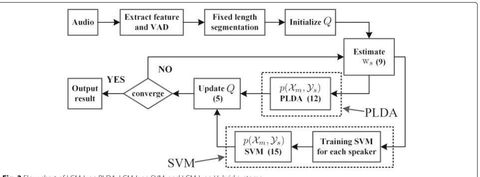
where κ is a scale factor set by experiments (κ = 1 in the PLDA setting). The explanation ofκ is similar to the κ of (1) in [47]. Asp(Xm)is the same forSspeakers and p(Ys,Xm|ims) = p(Xm)p(Ys|Xm,ims), thep(Xm) will be canceled in the following computation. The flow chart of LCM-Ivec-PLDA is shown in Fig.3without the flow path denoted as SVM.
4.2.2 SVM
Another discriminative option is using a support vector machine (SVM). After the estimation of ws, we train SVM models for all speakers. When training a SVM model (ηs,bs) with a linear kernel for speaker s, ws is regarded as a positive class and the other speakersωs(s = s) are regarded as negative classes.ηs,bsare linearly compressed weight and bias.
The SVM scoring is
sSVMms =ηswm+bs (15)
and the posterior probability withSspeaker constraint is
p(Ys|Xm,ims)∝
expκsSVMms
expκSs=1sSVMms
(16)
Fig. 3Flow chart of LCM-Ivec-PLDA, LCM-Ivec-SVM, and LCM-Ivec-Hybrid systems
following computation. The flow chart of LCM-Ivec-SVM is shown in Fig.3without the flow path denoted as PLDA.
4.2.3 Hybrid
The calculation ofp(Xm,Ys)is not explicitly specified in the LCM algorithm, which is just like the kernel function in SVM. As long as the kernel matrix satisfies the Mercer criterion [48], different choices may make the algorithm more discriminative and more generalized. In addition, multiple kernel learning is also possible by combining sev-eral kernels to boost the performance [49]. In the LCM algorithm, as long as the probability p(Xm,Ys) satisfies the condition that the more likely both Xm and Ys are from the same classs, the largerp(Xm,Ys)will be, we can take it and embrace more algorithms, e.g., the abovemen-tioned PLDA and SVM. We combine PLDA with SVM by iteration, see Fig.3. This iteration takes advantages of both PLDA and SVM and is expected to reach a better performance. This hybrid iterative system is denoted as LCM-Ivec-Hybrid system.
5 Further improvements
5.1 Neighbor window
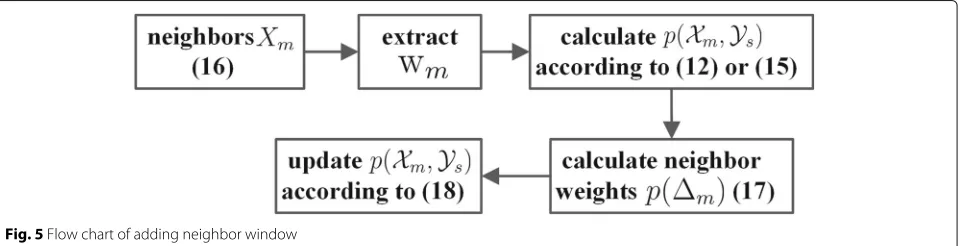
In fixed-length segmentation, each segment is usually very short to ensure its speaker homogeneity. However, this shortness will lead to inaccuracy when extracting seg-ment i-vectors and calculatingp(Xm,Ys). Intuitively, if a speakersappears at timem, the speaker will appear at a great probability in the vicinity of time m. So its neigh-boring segments can be used to improve the accuracy of p(Xm,Ys). We propose two methods of incorporat-ing neighborincorporat-ing segment information. At data level, we extract long-term segmental i-vectorXmto use the neigh-bor information. At score level, we build homogeneous Poisson point process model to calculatep(Xm,Ys).
Algorithm 2: LCM-Ivec-PLDA, LCM-Ivec-SVM, and LCM-Ivec-Hybrid
1: Voice activity detection and feature extraction 2: Segmentation
2.1: Split the audio into short segments equally, hence getMsegments.
3: Clustering
3.1: InitializeQrandomly 3.2:
Estimate speaker i-vector ws(10) based onQand xm 3.3: Extract each segment i-vector wm, see Section5 for more details.
3.4 (PLDA):
Calculate p(Xm,Ys) by PLDA (13) for each segment and speaker.
3.4 (SVM):
Train SVM for each speaker, and calcu-late p(Xm,Ys) by (16) for each segment and speaker.
3.4 (Hybrid): do 3.4 (PLDA) and 3.4 (SVM) alternatively
3.5: UpdateQaccording to (4). 3.6: Repeat 3.2–3.5 until converge.
5.1.1 Data level window
At the data level, we extract wmusing xmand its neighbor data. Let
Xm=
xm− Md,· · ·, xm,· · ·, xm+ Md
(17)
Fig. 4Data level and score level windows
be noted that Xm may contain more than one speaker, but this does not matter. This is because the extracted wm only represents the time m, not the time duration (m− Md,· · ·,m+ Md). From another aspect, data level window can be seen as a sliding window with high overlapping to increase the segmentation resolution.
5.1.2 Score level window
At the score level, we update p(Xm,Ys) with neighbor scores. Given the condition thatmth segment belongs to speakers, we consider the probability that(m+ m)th segment does not belong to speakers. If we define the appearance of a speaker change point as an event, the above process can be approximated as a homogeneous Poisson point process [50]. Under this assumption, the probability that a speech segment from m to m+ m belongs to the same speaker is equivalent to the probabil-ity that the speaker change point does not appear fromm tom+ m, and can be expressed as
p( m)=e−λ m, m≥0 (18)
where λ is the rate parameter. It represents the aver-age number of speaker change points in a unit time. We
consider the contribution of p(Xm+ m,Ys)to p(Xm,Ys) by updatingp(Xm,Ys)as follows:
p(Xm,Ys)← Ms
m=− Ms
p( m)p(Xm+ m,Ys)
(19)
where Ms is score level half window length, Ms > 0. It should be noted that, Md, Ms and λ are experiment parameters and will be exam-ined in the next section. As wm is extracted from Xm = (xm− Md,· · ·, xm+ Md), in fact, the updated p(Xm,Ys)is related to(xm− Ms− Md,· · ·, xm+ Ms+ Md), as shown in Fig.4. The full process of incorporating two neighbor windows is shown in Fig.5.
5.2 HMM smoothing
After several iterations, speaker diarization results can be obtained according toqms. However, the sequence infor-mation is not considered in the LCM system, there might be a number of speaker change points in a short duration. To address the frequent speaker change problem, a hidden Markov model (HMM) is applied to smooth the speaker change points. The initial probability of HMM isπs =
p(Ys). The self-loop transition probability isaii and the other transition probabilities areaij = 1S−−a1ii,i = j. Since the probability that a speaker transits to itself is much larger than that of changing to a new speaker, the self-loop probability is set to be 0.98 in our work. The emission probability is calculated based on PLDA (13) or SVM (16). With this HMM parameters,qmscan be smoothed using the forward-backward algorithm.
5.3 AHC initialization
Although random initialization works well in most cases, LCM and VB systems tend to assign the segments to each speaker evenly in the case where a single speaker dom-inates the whole conversation, leading to poor results. According to the comparative study [40], we know that the bottom-up approach will capture comparatively purer models. Therefore, we recommend an informative AHC initialization method, similar to our previous paper [51]. After using PLDA to compute the log likelihood ratio between two segment i-vectors [34, 35], AHC is applied to perform clustering. Using the AHC results, two prior calculation methods, hard prior and soft prior, are proposed [51].
5.3.1 Hard prior
According to the AHC clustering results, if a segmentmis classified to a speakers, we will assignqmswith a relatively larger valueq. The hard prior is as follows:
qms=I(Xm∈s)q+I(Xm∈/s) 1−q
S−1 (20)
whereI(·)is the indicator function.I(Xm∈s)means a segmentmis classified to speakers.
5.3.2 Soft prior
b For the soft prior, we first calculate the center of each estimated speakers
μws=
M
m=1I(xm∈s)wm M
m=1I(xm∈s)
(21)
The distance between wmandμwsisdms= wm−μws2. According to the AHC clustering results, if a segmentmis classified to a speakers, the prior probability for speakers at timemis
qms= 1 2
⎡ ⎢ ⎣e
− dms dmax,s
k −e−1 1−e−1 +1
⎤ ⎥
⎦ (22)
wheredmax,s =maxxm∈s(dms),kis a constant value. This soft prior probability varies from 0.5 to 1, ensuring that if wsis closer toμws,qmswill be larger. For other speakers at timem, the prior probability is(1−qms)/(S−1).
6 Related work and discussion
6.1 Core problem of speaker diarization
Different from some mainstream approaches, we take a different view for the basic concept of speaker diarization. Paper [40] summarizes that the task of speaker diarization is formulated as solving the following objective function:
argS,Gmaxp(S,G|X) (23)
where X is the observed data, S and G are speaker sequence and segmentation. In our work, we formulate the speaker diarization problem as follows:
argY,Qmaxp(X,Y,Q) (24)
where X be the observed data, Y and Q are hidden speaker representation and latent class probability matrix. Both objective functions can solve the problem of speaker diarization. However, the objective function (23) involves segmentation which introduces a premature hard decision that may degrade the system performance. The objective function (24) has difficulty in solving speaker overlapping problem and depends on the accurate estimate of speaker number.
6.2 Compared with VB
In VB,Ysis a speaker i-vector andp(Xm,Ys)is the eigen-voice scoring (Eq. (14in [2]), a generative model. In our paper, we replace eigenvoice scoring with PLDA or SVM scoring to compute p(Xm,Ys) which benefits from the discriminability of PLDA or SVM. Both VB and LCM-Ivec-PLDA/SVM are iterative processes, and there are two important steps:
Step 1 estimateQbased onX andY.
Step 2 estimateYbased onXandQ.
The two algorithms are almost the same in the second step. However, in step 1, the calculation ofQis more accu-rate by introducing the PLDA or SVM. In recent speaker recognition evaluations (e.g., NIST SREs), the Ivec-PLDA performed better than eigenvoice model (or joint factor analysis, JFA) [3]. The SVM is suitable for classification task with small samples. This is the reason why we intro-duce these two methods to LCM. Compared with VB, the main benefit of LCM-Ivec-PLDA/SVM is that it takes advantages of PLDA or SVM to improve the accuracy of p(Xm,Ys). Besides, the p(Xm,Ys) is enhanced by its neighbors both at the data and score level.
6.3 Compared with Ivec-PLDA-AHC
as done in paper [18,34–37]. Based on the PLDA similar-ity matrix, AHC is applied to the clustering task. Although the performance is improved, it still has the premature hard decision problem.
6.4 Compared with PLDA-VB
In paper [7], PLDA is combined with VB, and is similar to ours. We believe that the probabilistic-based iterative framework, as depicted in the LCM, and not just the introduction of PLDA, is the key to solving the prob-lem of speaker diarization. Our subsequent experiments also prove that using SVM can achieve a similar perfor-mance. The hybrid iteration inspired by the LCM can improve the performance further. In addition, we also study the use of neighbor information, HMM smoothing, and initialization method.
7 Experiments
Experiments have been implemented on five databases: NIST RT09 SPKD SDM (RT09), our own speaker imbal-anced TL(TL), LDC CALLHOME97 American English speech (CALLHOME97) [13], NIST SRE00 subset of the multilingual CALLHOME (CALLHOME00), and NIST SRE08 short2-summed (SRE08) databases to examine the performance of LCM. Speaker error (SE) and diariza-tion error rate (DER) are adopted as metrics to measure the system performance according to the RT09 evalua-tion plan [12] for RT09,TL, CALLHOME97, and CALL-HOME00 database. Equal error rate (EER) and minimum detection cost function (MDCF08) are adopted as auxil-iary metrics for SRE08 database.
7.1 Common configuration
Perceptual linear predictive (PLP) features with 19 dimen-sions are extracted from the audio recordings using a 25 ms Hamming window and a 10 ms stride. PLP and log-energy constitute a 20 dimensional basic feature. This base feature along with its first derivatives are concate-nated as our acoustic feature vector. VAD is implemented using the frame log-energy and subband spectral entropy. The UBM is composed of 512 diagonal Gaussian compo-nents. The rank of the total variability matrixTis 300. For the PLDA, the rank of the subspace matrix is 150. For seg-ment neighbors, Md, Ms andλ are 40, 40, and 0.05, respectively.
7.2 Experiment results with RT09
The NIST RT09 SPKD database has seven English meet-ing audio recordmeet-ings and is about 3 h in length. The BeamformIt toolkit [52] and Qualcomm-ICSI-OGI [53] front-end are adopted to realize acoustic beamforming and speech enhancement. We use Switchboard-P1, RT05, and RT06 to train UBM,T, and PLDA parameters. Three sets of experiments have been implemented to verify
the performance of our proposed LCM systems, usage of neighbor window, and HMM smoothing on RT09 database, respectively.
7.2.1 Comparison among different methods
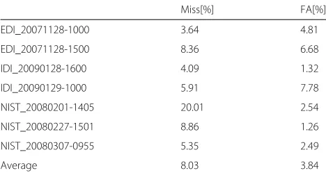
In the first set of experiments, we study the performance of different systems on the RT09 database. Table2lists the miss (Miss) rate and false alarm (FA) speech rate of LCM-Ivec-Hybrid system. It can be seen that the miss rate of the fifth recording reaches 20.0% percentage. This recording has much overlapping speech which is not well handled by our proposed approach.
Results of GMM-BIC-AHC, VB, and LCM-Ivec-PLDA/SVM/Hybrid systems are listed in Table 3. It can be seen that the performance of LCM systems is better than that of BIC system. This can be ascribed to the usage of qms for soft decisions instead of hard decisions. The performance of LCM is also better than VB system. This demonstrates that the introduction of a discriminative model is very effective. VB is a method with an iterative optimization based on a generative model. In contrast, LCM is a method with the computation of p(Xm,Ys) based on discriminative model, which is in line with the basic requirements of the speaker diarization task and contributes to its performance improvement. Compared with the classical VB system, the DER of LCM-Ivec-PLDA, LCM-Ivec-SVM, and LCM-Ivec-Hybrid have an average relative improvement of 23.5%, 27.1%, and 43.0% on NIST RT09 database. For some recordings, which already have good DERs with PLDA or SVM, the performance improvement of hybrid system is relatively small. For others with poorer DERs, the improvement of the hybrid system is prominent. We infer that the hybrid system may help to jump out of a local optimum achieved by a single algorithm.
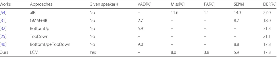
We also compare our system performance with other research work in the literature. Table4 lists the average performance of different methods on the RT09 database.
Table 2Miss and FA of LCM-Ivec-Hybrid system for RT09
Miss[%] FA[%]
EDI_20071128-1000 3.64 4.81
EDI_20071128-1500 8.36 6.68
IDI_20090128-1600 4.09 1.32
IDI_20090129-1000 5.91 7.78
NIST_20080201-1405 20.01 2.54
NIST_20080227-1501 8.86 1.26
NIST_20080307-0955 5.35 2.49
Average 8.03 3.84
Table 3Experiment results of different methods on RT09
DER[%] Speaker # BIC VB LCM-Ivec
PLDA SVM Hybrid
Given speaker # - Yes Yes Yes Yes Yes
EDI_20071128-1000 4 29.32 10.67 9.89 9.91 9.83
EDI_20071128-1500 4 35.61 48.66 19.68 19.87 17.40
IDI_20090128-1600 4 29.12 11.15 7.02 7.14 7.14
IDI_20090129-1000 4 37.27 35.85 31.99 32.37 21.82
NIST_20080201-1405 5 61.54 49.05 44.67 43.05 38.53
NIST_20080227-1501 6 40.32 39.97 24.76 25.66 13.96
NIST_20080307-0955 11 46.62 23.50 22.86 16.44 16.00
Average - 39.97 31.26 22.98 22.06 17.81
1The code for the BIC diarization system was downloaded from:https://github.com/gdebayan/Diarization_BIC
2VB is the system described in P. Kenny’s paper [2]. This system is partly realized by the python code downloaded from: http://speech.fit.vutbr.cz/software/vb-diarization-eigenvoice-and-hmm-priors
All of these systems except [54] is under a SDM condi-tion. It can be seen that the Miss + FA of our method is relatively higher. This is ascribed to the VAD error and overlapping speech. Our method has the lowest SE and DER.
7.2.2 Effect of different neighbor window
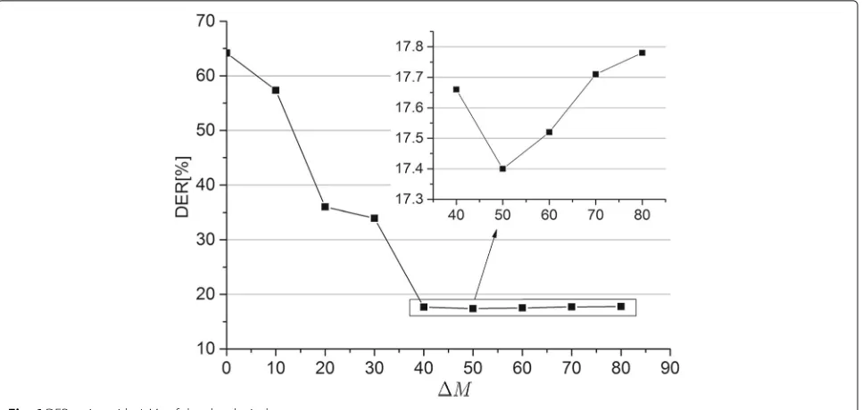
In the second set of experiments, we study the influ-ence of different neighbor windows at both data level and score level. For the data level window, Fig. 6shows the DER varies with Mdof LCM-Ivec-Hybrid on the audio ’EDI_20071128-1500’. It can be seen that when Md=0, that is to say no data level window is added, the per-formance of the speaker diarization is poor. As Md becomes larger, DER firstly decreases and then increases slightly. This is because we can extract more speaker infor-mation from Mdas it gets larger, but if it grows too large, it begins to mix with other speaker’s information.
At the score level, the DER varied with Ms andλis shown in Fig. 7. We can see that,whenλ approaches to 0, the value of (18) approaches 1, and the Poisson win-dow degrades to a rectangular winwin-dow, DER also first decreases and then increases with Ms. Asλgets larger, the window becomes sharper, so DER is not so sensitive to a larger Ms.
Table5shows the experimental results of the LCM sys-tem with or without neighbor windows on RT09. All these systems are randomly initialized. It can be seen that, from left to right, the performance of each system is gradually improved . This demonstrates that taking segment neigh-bors into account improves the robustness and accuracy of p(Xm,Ys) both in PLDA and LCM-Ivec-SVM systems, thus enhancing the system performance.
7.2.3 Effect of HMM smoothing
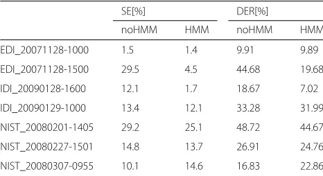
Table6lists our third set of experiment results, from the LCM-Ivec-PLDA system with or without HMM smooth-ing. It can be seen that, for the first six audio recordings, the SE and DER of the LCM-Ivec-PLDA system with HMM smoothing are better than that without HMM smoothing. This can be ascribed to the HMM smooth-ing that makes the speaker changes less frequent. For the seventh recording, the performance of LCM with HMM smoothing is not better than without HMM smoothing. This is because the seventh recording has eleven speakers, and the speaker changes much more frequently than in the first six examples. We guess that the HMM oversmooths the speaker change points, which means the loop proba-bility is too large for this case. In most cases, an HMM smoothing with proper parameters has positive effect.
Table 4Compared with other work performance on RT09. Scoring overlapped speech is accounted in the error rates
Works Approaches Given speaker # VAD[%] Miss[%] FA[%] SE[%] DER[%]
[54] aIB No – 11.6 1.1 14.3 27.0
[31] GMM+BIC No 2.7 – – 8.7 18.0
[32] BottomUp No 5.9 – – – 31.3
[25] TopDown No – – – – 21.1
[40] BottomUp+TopDown No 9.0 – – 8.8 17.8
Fig. 6DER varies with Mdof data level window
7.3 Experiment results withTL
The AHC initialization aims to solve of problem of speaker imbalance. When there is one speaker domi-nating the whole conversation (> 80% of the speech), VB and LCM will be sensitive to the initialization. Ran-dom initialization results in poor performance. But, if the conversation is not speaker imbalance, the initialization method has little influence on the performance. All the experiments except this section are random initialized.
The AHC initialization experiment is carried out on our collected audio recordingsTL. The training part of dataset TLcontains 57 speakers (30 female and 27 male). The total duration is about 94 h. All of the recordings are natural conversations (Mandarin) recorded in a quiet office condi-tion. The evaluation part ofTLhas three audio recordings (TL 7–9). These are also recorded in a quiet office, but there is one speaker who dominates the whole conver-sation (> 80% of the speech). Each recording has two
Table 5Performance of LCM system with or without neighbor windows
DER[%] LCM-Ivec-PLDA LCM-Ivec-SVM
neighbor window No Data Data+score No Data Data+score
EDI_20071128-1000 10.67 10.66 9.89 10.72 10.64 9.91
EDI_20071128-1500 45.14 20.93 19.68 43.02 20.77 19.87
IDI_20090128-1600 11.38 7.04 7.02 8.06 7.61 7.14
IDI_20090129-1000 34.00 32.11 31.99 33.19 32.24 32.37
NIST_20080201-1405 49.17 49.17 44.67 44.43 43.82 43.05
NIST_20080227-1501 58.49 47.11 24.76 27.01 26.18 25.66
NIST_20080307-0955 24.91 23.52 22.86 21.85 20.44 16.44
The term ‘no’ means no neighbor window is added, while ‘data’ means adding only data level window, and ‘data+score’ means that both data and score level windows are added
speakers and is about 20 min. In the AHC initialization,q is set to be 0.7 in the hard prior setting andkis 10 in the soft prior setting, unless explicitly stated. Table7lists the SE and DER after AHC initialization before applying VB or LCM diarization. The number of speakers is assumed to be known in advance.
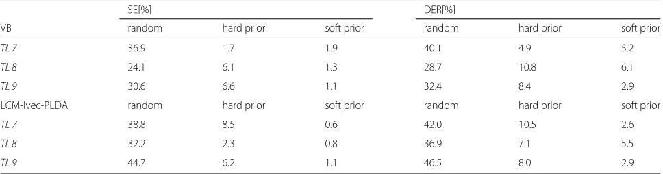
Figure8shows the DER of ’TL 7’ varies withkof soft prior (22). According to the variation trend, we choose k = 10 in our experiment. From Table8, we can see that random initialization gives poor results both in VB and LCM-Ivec-PLDA system in this case. The proposed AHC hard and soft prior improves the system performance significantly. The soft prior, which gives each segment an individual prior according to its distance to the esti-mated speaker centers, is more robust than the hard prior. With the AHC initialization, the LCM-Ivec-PLDA and VB system both have significant improvement compared with their random prior systems. The LCM-Ivec-PLDA system with hard/soft prior also surpasses the VB sys-tem with hard/soft prior with a relative improvement of 14.3%/14.2%. Tables7 and8demonstrate that, although AHC initialization gets a not bad result, adding VB or LCM further improve the performance.
Table 6Experiment result of LCM-Ivec-PLDA system with or without HMM smoothing
SE[%] DER[%]
noHMM HMM noHMM HMM
EDI_20071128-1000 1.5 1.4 9.91 9.89
EDI_20071128-1500 29.5 4.5 44.68 19.68
IDI_20090128-1600 12.1 1.7 18.67 7.02
IDI_20090129-1000 13.4 12.1 33.28 31.99
NIST_20080201-1405 29.2 25.1 48.72 44.67
NIST_20080227-1501 14.8 13.7 26.91 24.76
NIST_20080307-0955 10.1 14.6 16.83 22.86
7.4 Experiment results with CALLHOME97
The LDC CALLHOME97 American English speech database (CALLHOME97) consists of 120 conversations. Each conversation is about 30 min and includes about 10-min transcription. Only the transcribed parts are used. There are 109, 9, and 2 conversations containing 2, 3, and 4 speakers, respectively. We follow the practice of [55] and [56], conversations with 2 speakers are examined. We use Switchboard P1-3/Cell and SRE04-06 to train UBM, T, and PLDA parameters.
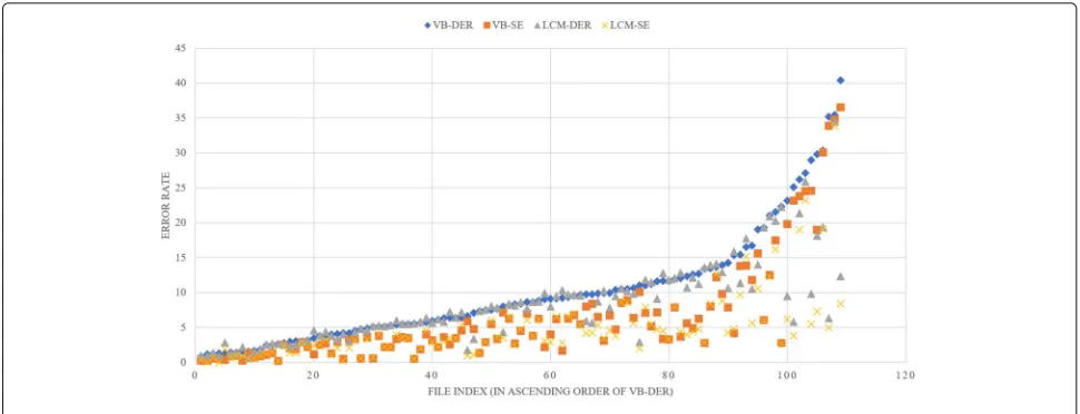
Scatter chart Fig. 9 enumerates VB-DER (blue dia-mond), VB-SE (orange square), LCM-Ivec-Hybrid-DER (LCM-DER, grey triangle), and LCM-Ivec-Hybrid-SE (LCM-SE, yellow cross) in the ascending order of DER. Both LCM-DER and LCM-SE are lower than VB-DER and VB-SE in summary, see also Table9.
We find an interesting thing. In the low region of DER (<6%), the performance of VB and LCM systems is sim-ilar. In the middle-to-high region of DER (>6%), LCM is not better than VB for all test conversations, but it has a significant performance improvement for a considerable number of conversations, see the distribution of blue dia-monds and grey triangles in Fig.9. The same situation is also reflected in Table3. We believe that the VB is trapped in a local optimum for these segments. By contrast, the LCM avoids this situation by incorporating with differ-ent methods. In addition, the standard deviation of DER and SE of the LCM is smaller (Table9), indicating that the performance of the LCM system is more stable.
Table 7Experiment result of AHC initialization
AHC initial SE[%] DER[%]
TL 7 3.0 5.9
TL 8 6.4 11.4
Fig. 8DER varies withkof soft prior (20)
Table9compares the results. It can be seen that com-pared with the VB system, the LCM-Ivec-Hybrid system has a relatively improvement of 26.6% and 17.3% in SE and DER, respectively. Compared with other listed methods, the LCM-Ivec-Hybrid system also performs best on the CALLHOME97 database. Diarization systems based on i-vector, VB, or LCM are trained in advance and perform well in fixed conditions. While diarization systems based on HDM have little prior training, it can perform better if test conditions vary frequently.
7.5 Experiment results with CALLHOME00
The CALLHOME00, a subtask of NIST SRE00, is a multi-lingual telephone database and consists of 500 recordings. Each recording is about 2∼5 min in duration, containing 2 ∼7 speakers. We use oracle speech activity marks and
speaker numbers. Similar to [34,38,57–59], overlapping error is not accounted. So, the DER is identical to the SE in this section. We use Switchboard P1-3/Cell and SRE04-06 to train UBM,T, and PLDA parameters.
From Table10, we may draw a conclusion that our pro-posed methods are optimal. However, it is not fair for [34, 57–59]. Paper [57, 59] do not use the oracle VAD, and paper [34,57,58] do not use the oracle speaker number. And both two factors have a great influence on the sys-tem performance. These results can only be used as an auxiliary reference. Paper [38] has the same setting with our work, and the proposed LCM-Ivec-Hybrid is slightly better. Based on the results of above three sections, we guess that our proposed system is more suitable for long speech, for the reason that Ys can be estimated more accurately from the long speech.
Table 8Experiment result with random initialization and AHC initialization
SE[%] DER[%]
VB random hard prior soft prior random hard prior soft prior
TL 7 36.9 1.7 1.9 40.1 4.9 5.2
TL 8 24.1 6.1 1.3 28.7 10.8 6.1
TL 9 30.6 6.6 1.1 32.4 8.4 2.9
LCM-Ivec-PLDA random hard prior soft prior random hard prior soft prior
TL 7 38.8 8.5 0.6 42.0 10.5 2.6
TL 8 32.2 2.3 0.8 36.9 7.1 5.5
Fig. 9DER and SE of VB and LCM-Ivec-Hybrid on CALLHOME97 database
7.6 Experiment results with SRE08
The NIST SRE08 short2-summed channel telephone data consists of 1788 models and 2215 test segments. Each segment is about 5 min in duration (about 200 h in total). We find that there is no official speaker diariza-tion key for the summed data. Thus, neither DER or SE is adopted for this set of experiments. The paper [2] reports that “We see that there is some correla-tion between EER and DER, but this is relatively weak.” So, we measure the effect of diarization through EER and MDCF08 in an indirect way. On the one hand, we use the NIST official trials (summed, short2-summed-eng). On the other hand, we follow the practice of [60] and make extended trials (ext-short2-summed, ext-short2-summed-eng).
We use Switchboard P1-3/Cell and SRE04-06 to train UBM,T and PLDA parameters. Here, our speaker veri-fication system is a traditional GMM-Ivec-PLDA system. The extracted 39 dimension PLP feature has 13 dimen-sion static feature, and . A diagonal GMM with 2048 components is gender-independent. The rank of the total variability matrixTis 600. For the PLDA, the rank of the subspace matrix is 150 [44].
To begin with, we give some experimental results on the NIST SRE08 core tasks, i.e., short2-short3-telephone (short2-short3) and short2-short3-telephone-English tri-als (short2-shor3-eng), to verify the performance of above speaker verification system, see Table11. Compared with the classical paper [42], our results are normal. Subse-quently, we present results of the same speaker verifica-tion system on the NIST SRE08 short2-summed condi-tion. Without the front diarization, the EER and MDCF08 are as high as 16.94% and 0.686. Whether it is a VB + windows or LCM-Ivec-Hybrid, speaker diarization can
significantly improve system performance. Comparing case 5,9,14,17 with case 6,10,15,18 in Table11, we think that the performance improvement of LCM over VB is mainly due to the better diarization of LCM.
According to our literature research, there are few doc-uments that report EER and MDCF08 on the short2-summed condition. We list state-of-the-art diarization-verification systems developed by the LPT [61,62] in 2008 in Table11. Paper [2] also presents the related EER in its Fig.4. Compared with them, our system works better. Part of the reason is the advance of speaker verification system, and the other part is the effectiveness of our proposed methods.
Paper [60] gives results on the extended trials which is more convincing in our opinion. On the ext-short2-summed trials, although our EER (4.99%) is worse than their report (4.39%), but our MDCF08 (0.201) is better than their report (0.209). Besides, paper [60] is a fusion system but our work is a single system.
8 Conclusion
In this paper, we have applied a latent class model (LCM) to the task of speaker diarization. LCM provides a
frame-Table 9Comparison with other works on CALLHOME97 database
Works Method SE[%] DER[%]
[55] Hidden distortion models (HDM)
– 12.71
[56] GMM-Ivec – 9.8
[2] + ours VB + windows 6.58±7.59 10.08±8.09
Table 10Result (in DER[ %]) on CALLHOME00 database
Speaker # 2 (303) 3 (136) 4 (43) 5 (10) 6 (6) 7 (2) Average
Table2in [57] 8.7 15.7 15.1 20.2 25.5 29.8 11.67
Figure5in [38] * 5.0 12.5 17.7 20.5 21.5 33.1 8.75
Table5in [58] 7.5 11.8 14.9 22.8 25.9 26.9 9.91
[34] – – – – – – 13.7
Kaldi [59] – – – – – – 8.69
VB+windows 6.68 14.51 18.68 26.78 24.88 25.35 10.53
LCM-Ivec-Hybrid 4.26 13.12 17.96 25.74 24.70 25.35 8.60
() denotes the number of recordings
* reflects that these numbers are measured from figures
work that allows multiple models to compute the prob-ability p(Xm,Ys). Based on this algorithm, additional LCM-Ivec-PLDA, LCM-Ivec-SVM and LCM-Ivec-Hybrid systems are introduced. These approaches significantly outperform traditional systems.
There are five main reasons for this improvement: (1) introducing a latent class model to speaker diariza-tion and using discriminative models in the computa-tion ofp(Xm,Ys) which enhances the system’s ability at distinguishing speakers. (2) Incorporating temporal con-text through neighbor windows, which increases speaker information extracted from each short segment. This
incorporation is used both at the data level, takingXmand its neighbors to constituteXm when extracting Ym, and at the score level, considering the contribution of neigh-bors when calculating p(Xm,Ys). 3) Performing HMM smoothing, which takes the audio sequence information into consideration. (4) AHC initialization is also a cru-cial factor when the conversation is dominated by a single speaker. (5) The hybrid schema can avoid the algorithm falling into local optimum in some cases.
Finally, our proposed system has the best overall perfor-mance on NIST RT09, CALLHOME97, CALLHOME00, and SRE08 short2-summed database.
Table 11Results on NIST SRE08 summed channel telephone data
Case Trials (Ivec-PLDA) Diarization EER[%] MDCF08
1 Short2-short3 – 4.47 0.245
2 Short2-summed – 16.94 0.686
3 Short2-summed Figure4in [2] 9.0 –
4 Short2-summed LPT [61,62] – 0.493
5 Short2-summed VB + windows 9.64 0.410
6 Short2-summed LCM-Ivec-Hybrid 8.71 0.374
7 Ext-short2-summed – 10.77 0.438
8 Ext-short2-summed Table2in [60] 4.39 0.209
9 Ext-short2-summed VB + windows 5.48 0.228
10 Ext-short2-summed LCM-Ivec-Hybrid 4.99 0.201
11 Short2-short3-eng – 1.76 0.0895
12 Short2-summed-eng – 14.25 0.504
13 Short2-summed-eng LPT [61,62] – 0.282
14 Short2-summed-eng VB + windows 6.33 0.236
15 Short2-summed-eng LCM-Ivec-Hybrid 5.62 0.245
16 Ext-short2-summed-eng – 10.00 0.400
17 Ext-short2-summed-eng VB + windows 4.13 0.154
Endnote
1Note that, equal prior is assumed in (15) in [2].
Acknowledgements
We would like to thank the editor and anonymous reviewers for their careful work and thoughtful suggestions that have helped improve this paper substantially.
Authors’ contributions
The contributions of each author are as follows: LH proposed the LCM methods, score level windowing, and the AHC initialization for speaker diarization. He realized these systems in C++ code (Aurora3 Project) and wrote the paper. XC did a lot of literature research, wrote the section of mainstream approaches and algorithms, and studied the data level windowing and HMM smoothing. CX did experiments on the database based on the code provided by He Liang. He also recorded and analyzed the results. YL provided the comparative systems. JL gave some advices. MTJ checked the whole article and polished English language usage.
Funding
The work was supported by the National Natural Science Foundation of China under Grant No. 61403224.
Availability of data and materials
The CALLHOME00, NIST RT05/RT06/RT09, and NIST SRE08 database were released by NIST during evaluation. The abovementioned data and LDC CALLHOME97 can also be obtained by LDC (https://www.ldc.upenn.edu/). For the TL database, please contact author for data requests
Ethics approval and consent to participate Not applicable.
Consent for publication Not applicable.
Competing interests
The authors declare that they have no competing interests.
Author details
1Department of Electronic Engineering, Tsinghua University, Zhongguancun
Street, 100084 Beijing, China.2Electrical and Computer Engineering, University
of Kentucky, 453E FPAT, Lexington, KY, 40506-0046, USA.
Received: 29 August 2018 Accepted: 28 May 2019
References
1. X. A. Miro, S. Bozonnet, N. Evans, C. Fredouille, G. Friedland, O. Vinyals, Speaker diarization: a review of recent research. IEEE Trans. Audio Speech Lang. Process.20(2), 356–370 (2012).https://doi.org/10.1109/TASL.2011. 2125954
2. P. Kenny, D. Reynolds, F. Castaldo, Diarization of telephone conversations using factor analysis. IEEE J. Sel. Top. Signal Proc.4(6), 1059–1070 (2010). https://doi.org/10.1109/JSTSP.2010.2081790
3. P. Kenny, Bayesian analysis of speaker diarization with eigenvoice priors. Technical report, CRIM (2008)
4. D. Reynolds, P. Kenny, F. Castaldo, inProceedings of Interspeech 2009. A study of new approaches to speaker diarization (ISCA(International Speech Communication Association), Brighton, 2009), pp. 1047–1050 5. F. Valente, Variational bayesian methods for audio indexing. PhD thesis,
Eurecom, Sophia-Antipolis, France (2005). http://dx.doi.org/10.5075/epfl-thesis-2092.http://www.eurecom.fr/publication/1739
6. M. Diez, P. M. L. Burget, inOdyssey The Speaker and Language Recognition Workshop. Speaker diarization based on bayesian hmm with eigenvoice priors (ISCA, Les Sables d’Olonne, 2018), pp. 147–154
7. A. E. Bulut, H. Demir, Y. Z. Isik, H. Erdogan, in2015 IEEE International Conference on Acoustics, Speech and Signal Processing (ICASSP). Plda-based diarization of telephone conversations (IEEE, Brisbane, 2015),
pp. 4809–4813.https://doi.org/10.1109/ICASSP.2015.7178884
8. P. F. Lazarsfeld, N. W. Henry,Latent Structure Analysis. (Houghton Mill, Boston, 1968)
9. J. Magidson, J. K. Vermunt, Latent class models for clustering: A comparison with kmeans. Can. J. Mark. Res.20, 37–44 (2002) 10. L. M. Collins, S. T. Lanza,Latent Class and Latent Transition Analysis with
Applications in the Social, Behavioral, and Health Sciences, 1st edn. (Wiley, New York, 2009)
11. K. J. Han, S. S. Narayanan, inProceedings of Interspeech 2007. A robust stopping criterion for agglomera-tive hierarchical clustering in a speaker diarization system (ISCA, Antwerp, 2007), pp. 1853–1856
12. NIST, The 2009 (RT-09) Rich Transcription Meeting Recognition Evaluation Plan (2009). Available: https://www.nist.gov/itl/iad/mig/rich-transcription-evaluation
13. L. data consortium, LDC97S42, Catalog (1997). Available:http://www.ldc. upenn.edu/Catalog/catalogEntry.jsp?catalogIdDLDC97S42. Accessed 29 Aug 2018
14. M. Zelenák, H. Schulz, J. Hernando, Speaker diarization of broadcast news in albayzin 2010 evaluation campaign. EURASIP J. Audio Speech Music Process.2012(1), 19 (2012).https://doi.org/10.1186/1687-4722-2012-19 15. C. Wooters, M. Huijbregts,TheICSIRT07sSpeakerDiarization System. (R. Stiefelhagen,
R. Bowers, J. Fiscus, eds.) (Springer, Berlin, Heidelberg, 2008), pp. 509–519 16. V. Gupta, G. Boulianne, P. Kenny, P. Ouellet, P. Dumouchel, in2008 IEEE
International Conference on Acoustics, Speech and Signal Processing. Speaker diarization of french broadcast news, (2008), pp. 4365–4368. https://doi.org/10.1109/ICASSP.2008.4518622
17. S. Meignier, T. Merlin, inCMU SPUD Workshop. Lium spkdiarization: an open source toolkit for diarization (HAL, Dallas, 2010)
18. B. Desplanques, K. Demuynck, J.-P. Martens, inProceedings of Interspeech 2015. Factor analysis for speaker segmentation and improved speaker diarization (ISCA, Dresden, 2015), pp. 3081–3085
19. S. Jothilakshmi, V. Ramalingam, S. Palanivel, Speaker diarization using auto associative neural networks. Eng. Appl. Artif. Intell.22(4), 667–675 (2009). https://doi.org/10.1016/j.engappai.2009.01.012
20. V. Gupta, in2015 IEEE International Conference on Acoustics, Speech and Signal Processing (ICASSP). Speaker change point detection using deep neural nets (IEEE, Queensland, 2015), pp. 4420–4424.https://doi.org/10. 1109/ICASSP.2015.7178806
21. M. Hruz, Z. Zajic, in2017 IEEE International Conference on Acoustics, Speech and Signal Processing (ICASSP). Convolutional neural network for speaker change detection in telephone speaker diarization system (IEEE, New Orleans, 2017), pp. 4945–4949
22. Z. Zajic, M. Hruz, L. Muller, inProceedings of Interspeech 2017. Speaker diarization using convolutional neural network for statistics accumulation refinement (ISCA, Stockholm, 2017), pp. 3562–3566
23. H. Bredin, in2017 IEEE International Conference on Acoustics, Speech and Signal Processing (ICASSP). Tristounet: Triplet loss for speaker turn embedding (IEEE, New Orleans, 2017), pp. 5430–5434
24. R. Yin, H. Bredin, C. Barras, inProceedings of Interspeech 2017. Speaker change detection in broadcast tv using bidirectional long short-term memory networks (ISCA, Stockholm, 2017), pp. 3827–3831 25. S. Bozonnet, N. W. D. Evans, C. Fredouille, in2010 IEEE International
Conference on Acoustics, Speech and Signal Processing (ICASSP). The lia-eurecom rt’09 speaker diarization system: Enhancements in speaker modelling and cluster purification (IEEE, Dallas, 2010), pp. 4958–4961. https://doi.org/10.1109/ICASSP.2010.5495088
26. I. Lapidot, J.-F. Bonastre, inOdyssey The Speaker and Language Recognition Workshop. On the importance of efficient transition modeling for speaker diarization (ISCA, Singapore, 2012), pp. 138–145
27. I. Lapidot, J.-F. Bonastre, inProceedings of Interspeech 2016. On the importance of efficient transition modeling for speaker diarization (ISCA, San Francisco, 2016), pp. 2190–2193
28. R. Milner, T. Hain, inProceedings of Interspeech 2016. Dnn-based speaker clustering for speaker diarisation (ISCA, San Francisco, 2016), pp. 2185–2189
29. M. Najafian, J. H. L. Hansen, in2017 IEEE International Conference on Acoustics, Speech and Signal Processing (ICASSP). Environment aware speaker diarization for moving targets using parallel dnn-based recognizers (IEEE, New Orleans, 2017), pp. 5450–5454.https://doi.org/10. 1109/ICASSP.2017.7953198