R E S E A R C H A R T I C L E
Open Access
A robust algorithm for implicit description
of immersed geometries within a
background mesh
Daniel Baumgärtner
1*, Johannes Wolf
1, Riccardo Rossi
2, Pooyan Dadvand
2and Roland Wüchner
1*Correspondence:
1Technische Universität
München, Arcisstr. 21, 80333 München, Germany Full list of author information is available at the end of the article
Abstract
The paper presents a robust algorithm, which allows to implicitly describe and track immersed geometries within a background mesh. The background mesh is assumed to be unstructured and discretized by tetrahedrons. The contained geometry is assumed to be given as triangulated surface. Within the background mesh, the immersed geometry is described implicitly using a discontinuous distance function based on a level-set approach. This distance function allows to consider both, “double-sided” geometries like membrane or shell structures, and “single-sided” objects for which an enclosed volume is univocally defined. For the second case, the discontinuous distance function is complemented by a continuous signed distance function, whereas ray casting is applied to identify the closed volume regions. Furthermore, adaptive mesh refinement is employed to provide the necessary resolution of the background mesh. The proposed algorithm can handle arbitrarily complicated geometries, possibly containing modeling errors (i.e., gaps, overlaps or a non-unique orientation of surface normals). Another important advantage of the algorithm is the embarrassingly parallel nature of its operations. This characteristic allows for a straightforward parallelization using MPI. All developments were implemented within the open source framework “KratosMultiphysics” and are available under the BSD license. The capabilities of the implementation are demonstrated with various application examples involving practice-oriented geometries. The results finally show, that the algorithm is able to describe most complicated geometries within a background mesh, whereas the approximation quality may be directly controlled by mesh refinement.
Keywords: Immersed boundary method, Implicit geometry description, Embedded geometry, Boundary tracking, Distance function, Level-set approach, Local best-fit approximation, Ray casting, Adaptive mesh refinement
Introduction
The increasing maturity of numerical techniques allows to perform detailed mechanical simulations taking into account geometrically complex, possibly moving objects, provided that asuitable computational mesh is available throughout the simulation. Unfortunately the availability of such a mesh is becoming more and more a bottleneck as the geometric complexity increases. Consider, for example, a situation in which the flow around an object shall be computed. Following classical approaches, the corresponding fluid domain
©The Author(s) 2018. This article is distributed under the terms of the Creative Commons Attribution 4.0 International License (http://creativecommons.org/licenses/by/4.0/), which permits unrestricted use, distribution, and reproduction in any medium, provided you give appropriate credit to the original author(s) and the source, provide a link to the Creative Commons license, and indicate if changes were made.
would be discretized by a “body-fitted” mesh, i.e., a mesh which matches the boundaries of the object. The requirement to locally match the boundaries, however, is problematic when the object represents a complicated geometry, say a complete racing car, or when the object contains many fine details, like the hole of a screw. In such cases, a proper resolution of the boundary can require a lot of manual modeling effort or lead to an impractical high mesh density. The corresponding limitations may be easily understood by trying out quality open source mesh generators like [1–5].
The situation becomes even worse when moving objects need to be taken into account, like in problems of fluid-structure interaction. In these cases, the requirement to main-tain a body-fitted mesh results in heavy mesh update procedures, which eventually will fail when large movements and rotations are involved. Furthermore, the simulation of problems with changing topology (like in the flow simulation of the landing gear of an aircraft during deployment) becomes virtually impossible, since the mesh graph changes. “Immersed boundary methods” appear to be a possible remedy to such problems. The general idea of immersed boundary methods is to place a model of the object of interest directly into a given background mesh, identify the object’s boundaries relative to the background mesh, and use the background mesh along with the implicit description of the immersed boundaries to eventually perform a mechanical analysis. The advantage is, that no body-fitted mesh is required anymore giving rise to a significantly decreased modeling effort. On the other hand, such an operation causes an intersection between the computational domain, i.e., the background mesh, and the objects’ skin. Correspondingly, algorithms are required to identify these intersections and to describe the immersed object implicitly.
It is obvious, that such an implicit geometrical representation of the object strongly depends on the grid size of the background mesh. That is, a too coarse mesh cannot represent the immersed object as accurately as a body-fitted mesh and geometrical details will be lost unless a local refinement is performed. However, this property is not necessarily bad, but can be exploited to run simulations with an intentionally reduced level of fidelity, as it is e.g. done in the context of the multiresolution paradigm.
Many approaches to perform computations based on an immersed boundary method were developed over the years. In the field of CFD, a review of immersed boundary meth-ods is given by [6]. An extended formulation to consider fluid-structure interaction is presented in [7]. More recent developments focusing on the finite element method are described in [8–11]. And an example in the context of the finite volume method is given by [12]. In the field of structural mechanics, the finite cell method (FCM) relies on an immersed boundary formulation [13,14]. An earlier proposition to represent solids in a structured background mesh is elaborated in detail in [15].
Besides the approaches above, which mostly focus on volumetric objects, the recently proposed isogeometric B-Rep analysis (IBRA) uses similar ideas to analyze thin-walled structures described as trimmed geometries in CAD. In IBRA, the geometry under consid-eration, representing e.g. a membrane or a shell, is immersed into an underlying NURBS-surface patch and the actual geometry is described by the cut-out of an arbitrarily curved free-form shape [16–18].
reconstruction of geometries that are immersed within a background mesh. In general, such an algorithm represents the basis of immersed boundary methods.
We consider the case of unstructured tetrahedral meshes, intersected by immersed objects given in form of triangulated surfaces. The immersed geometry is described implicitly using a discontinuous distance function based on a level-set approach. This allows to consider both, “double-sided” geometries, like sails, where fluid flows on both sides, and “single-sided” objects, for which an enclosed volume is univocally defined. For the second case, the discontinuous distance function is complemented by a continuous signed distance function. In this case, the identification of “inside” and “outside” regions, associated to respectively a positive and negative distance, is done by employing a ray casting approach. The ray casting is improved by using a cascade of techniques in order to enhance its robustness when dealing with “dirty” geometries. Furthermore, an adaptive mesh refinement, based on the technique described in [19], is employed to provide the necessary or intended resolution of the background mesh.
The proposed approach allows handling arbitrarily complicated geometries, possibly containing modeling errors (gaps, overlaps or a non-unique orientation of surface nor-mals). An important advantage over alternatives is the embarrassingly parallel nature of the operations involved, which allows a straightforward parallelization using MPI, provided that a copy of the object skin is owned by each of the MPI domains. All of the developments in current work were implemented and tested within the framework KratosMultiphysics [20,21] and are available under the BSD license [22].
Despite the focus on the implicit geometry description in this paper, it should be noted, that special attention is required if the proposed approach, with its included discontinuous distance function, is to be employed for the solution of physical problems. As a detailed discussion of the corresponding implications is far beyond the scope of this paper, but of interest especially in a finite element context, the situation in this case shall be briefly commented in the following.
The use of a discontinuous distance function inevitably implies that the finite element space is not conforming across cut faces. To consider this non-conformity, special strate-gies are typically employed in the formulation of conditions along the immersed bound-aries. A discussion of these strategies is not subject of this paper, but one can readily conclude that their formulation is a non-trivial task, particularly since it is difficult to discretize the immersed boundary for integration purposes. However, it is worthwhile to note, that the area of non-conformity tends to zero for smooth surfaces and an infinitely refined background mesh. In this context, the authors found, that applying boundary con-ditions based on discontinuous shape functions without any additional treatment of the non-conformity may be an effective approach in the solution of physical problems, even though a variational crime is committed. E.g., studies of the authors with a flow solver uti-lizing discontinuous shape functions as described in [23] show results in agreement with published data from general CFD analysis. This, however, is by no means a general result and different strategies will need to be devised when alternative solvers or formulations are employed.
points is then described in “Octree-based spatial search to determine intersections” sec-tion. Using the information about intersected elements, the actual representation of the immersed geometry by a discontinuous distance function is discussed in “Geometrical representation of immersed objects using a discontinuous distance function” section. In this section, also the related challenges are systematically prepared and specific solution approaches are elaborated. For an efficient improvement of the implicit geometry repre-sentation, local refinement strategies are presented in “Refinement strategies to improve the approximation quality” section. In “Identification of closed regions using a continu-ous distance function” section, an additional continucontinu-ous distance function is introduced, which is required for inside-outside distinctions in case of enclosed volumes. Finally, in “Examples of immersed geometries with different features and challenges” section, the developed and implemented concepts are demonstrated in various application examples each having its own challenges with respect to the immersed geometry.
Implicit geometry representation by means of a level-set approach
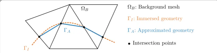
In this paper, we consider the case in which a geometry described by a triangulated surface is immersed into an unstructured tetrahedral background mesh. The objective is to implicitly describe the immersed geometry with respect to the background mesh, whereas particular focus is on the possibility to handle arbitrarily complicated geometries. The key idea to be leveraged is, that any tetrahedron in the background mesh can be intersected by the immersed geometry at most through a plane (which is not the case, e.g., for hexahedrons). Furthermore, it is assumed, that in cases where a given tetrahedron is intersected in a pattern that does not exactly form such a cutting plane, it may be properly approximated, e.g., by best-fit techniques. Given a description of the cutting plane for every intersected tetrahedron, it is finally possible to reconstruct an approximation of the immersed geometry.
To describe the cutting planes and hence the immersed geometry, a so called “level-set approach”, as described in [24], is utilized. The latter provides an implicit definition of the geometry as the zero isosurface of a smooth function defined over the background mesh. Typically, this function is chosen as thesigneddistance to the geometry of interest, whereas the sign is defined to be negative on one side of the geometry and positive on the other. The idea of such a distance function is visualized in Fig.1. In the figure, the distance function associates to each node of the background mesh the closest signed distance to the given immersed geometry. The sign may be chosen according to the normal orientation of the immersed geometry. The immersed geometry then appears as the zero distance isosurface.
Fig. 1 Distance function to implicitly describe an immersed geometry
Fig. 2 Need for a discontinuous distance function when dealing with arbitrary complicated geometries due to a potential non-unique definition of signed distances
given geometries, it must have a negative signed distance when considered as a part ofE2 and a positive signed distance as a part ofE1, which is obviously impossible.
In order to successfully capture such exceptions and to be able to describe arbitrarily complicated geometries, a distance function is used, which isdefined on an purely ele-mental basis. That is, the distances are computed individually for each element of the background mesh rather than for each node. This elemental description implies that the very same node may have different distance values when considered as part of different elements. The concept of an element-wise computation of distances is illustrated in Fig. 3. This customization gives rise to a central characteristic of our approach: The approx-imation of the immersed geometry turns into a purely local operation and the distance function becomesdiscontinuousalong the immersed boundary.
Fig. 3 Element-wise computation of distances
approximation of the cutting plane within each tetrahedron. Note also, that by having a purely local operation the distances can be computed independently for all elements in the background mesh. A parallelization of the approach is hence straight-forward and very effective, which is beneficial in terms of computational efficiency. Also, as seen later, the inherent discontinuities arising in the representation of the immersed geometry may be considered as negligible assuming a sufficiently refined background mesh. Given only a coarse mesh, choices of possible refinement strategies are described in “Refinement strategies to improve the approximation quality” section.
In the special case of dealing with closed geometries immersed in a background mesh, it is typically also required to determine which nodes of the background mesh are lying inside the closed regions and which ones are outside. In this special case, a continuous distance function is well defined and may be readily used to compute signed distances such that a negative distance indicates a point inside and a positive sign a point outside of the closed region. Therefore, in cases including closed immersed geometries, a continuous distance function is reconstructed on the basis of the above mentioned discontinuous one. A ray casting approach is then used to assign the resulting nodal distances with a sign. The latter appears to be the most robust solution, as it is detailed in “Identification of closed regions using a continuous distance function” section.
In summary, the proposed strategy to implicitly represent immersed geometries inside a background mesh is as follows: first, the immersed geometry is described element-wise by distances to the locally approximated cutting plane. This process corresponds to the formulation of a discontinuous distance function. If the problem involves complicated geometries, adaptive mesh refinement is applied prior to this step. Then, in case the immersed geometry contains closed bodies, the discontinuous distance function is com-plemented by a continuous one such that signed nodal distances may be determined. After computing both distance functions, the immersed geometry is finally described implicitly with respect to the background mesh and it may be readily reconstructed on the basis of the given distance values. The process is summarized in Fig.4. The following chapters will detail each individual step of this overall process. The corresponding chapters are referenced in the figure.
Octree-based spatial search to determine intersections
Input: background tet-mesh & triangulated surface geometry (e.g. stl)
Compute elemental distances using discontinuous distance function Refine background mesh if nessecary (5)
Output: Implicit geometry description with respect to the background mesh Closed geometry included?
Compute signed nodal distances using continous distance function (6)
Determine sign of nodal distances using ray casting Construct continous from discontinuous distance function
Y
N Tet intersects geometry? (3)
Loop over all tets
Determine local cutting plane (4)
For each tet node compute distance to cutting plane (4) Y
N
Fig. 4 Algorithm for implicit geometry description based on a combined discontinuous and continuous distance function (sections containing further details are referenced in brackets)
In the present work, it is necessary to find all intersecting elements of the immersed geometry for a given element of the background mesh. For that matter, it is valid to assume that the background mesh is modeled as a convex hull over the immersed geometry so thatNb>Ng, whereNbandNgare the number of background and geometry elements,
respectively. In a straightforward algorithm, to identify all intersections, every geometry element may be checked against each element of the background mesh corresponding to an algorithm of complexityO(Nb×Ng). For a highly refined background mesh this
quickly leads to an explosion of the computational costs. This calls for more advanced spatial search techniques.
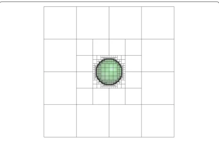
Fig. 5 Distribution of leaf cells resulting from a quadtree data structure generated around a circular geometry using eight consecutive levels of refinement
Since in the present case objects have to be searched in a very irregular domain, i.e., given an element of the background mesh it is necessary to search the intersecting elements of the immersed geometry, whereas the immersed geometry itself can be arbitrarily shaped and hence represent a very irregular domain, spatial search based on an octree appeared to be the best solution. In this method, a block-shaped bounding box around the immersed geometry is divided into eight equal cells, where each cell is partitioned into another eight cells in case that an element of the immersed geometry is contained. This process is performed several times up to the desired level of refinement. The final distribution of cells is then referred to as the leaf cells. As a result, the domain of the geometry is represented by a tree-like data structure, i.e., an octree in 3D or a quadtree in 2D. An example for the distribution of leaf cells resulting from a quadtree data structure is given in Fig.5. There are many partitioning techniques of this type [31]. In this work a mid-point partitioning based on the work of [32] has been employed as basic data structure.
Having identified a suitable data structure, the following general procedure is proposed to perform spatial search: First, the basic octree data structure representing the immersed geometry is created. Then, every element of the background mesh is assigned with point-ers to the corresponding leaf cells it intpoint-ersects with. Based on this link of information from both domains, the intersection testing between the immersed geometry and the background mesh can be eased significantly. Instead of checking every element of the background mesh against each element of the immersed geometry, one checks for a given background element just a small subset of all geometry elements for potential intersec-tions. This reduces the complexity of the intersection test from originallyO(Nb×Ng) to
an order ofO(Nb×log(Ng)).
Input: background tet-mesh & triangulated surface geometry
Search for subset of leaf cells inersecting tet
Generate bounding box around tet
Cell intersects tet (box-tet intersection)?
Generate octree based on immersed geometry
Output: Intersections between brackground mesh & immersed geometry Loop over tet elements of background mesh
Determine intersections between tet & geometry in subset of leaf cells Y
Determine leaf cells intersecting bounding box (box-box intersection)
Loop over intersecting leaf cells
Add cell to container N
Loop over tet edges
Check intersections between triangle & tet edge (triangle-line int.) Loop over leaf cells in container
Loop over triangles in leaf cell
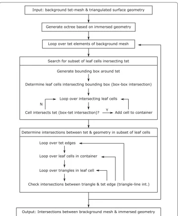
Fig. 6 Algorithm based on an octree data structure to determine intersection points between background mesh and immersed geometry
At first, an octree representing the immersed geometry is created and a loop over the elements of the background mesh is initialized.
Fig. 7 Approximation of an immersed geometry within each intersected element of a background mesh
Fig. 8 Signed nodal distance values defining cutting plane for an intersected element as zero isosurface. The cutting plane locally approximates the immersed geometry (blue area)
of leaf cells containing all (triangular) geometry elements with a possible intersection is obtained. This set is stored in a container and associated to the given background element. Given this container for an element of the background mesh, one can in the last main step identify the actual intersection points. As the detection of intersection points between a tetrahedron and a triangle is a geometrically complex problem, this step is divided into a loop over several basic tests. In these basic tests, the intersection points are deter-mined subsequently by testing all tetrahedron edges against the given triangles, which only involves a basic computation of the intersection point between a ray and a triangle. Having performed this last main step for all elements of the background mesh in the loop, all intersection points with the immersed geometry are finally determined.
Geometrical representation of immersed objects using a discontinuous distance function
In “Implicit geometry representation by means of a level-set approach” section the gen-eral approach to implicitly represent immersed objects within a background mesh was introduced. In this context, a tetrahedral background mesh and a triangulated immersed geometry is assumed. The corresponding algorithm is summarized in Fig.4. This chapter discusses in detail how to compute the elemental distances within the algorithm. Also it presents a way to visualize the corresponding approximation of the immersed geometry. This visualization will be the basis for the discussion of the approximation quality.
Computation of elemental distances
work, the arbitrary boundary of an immersed object is represented by a collection of pla-nar cutting planes, whereas in each intersected element of the background mesh there is exactly one defined plane. The principle is conceptually illustrated in Fig.7. As a conse-quence of this local reduction of the immersed geometry to a cutting plane, the approxi-mation quality is strictly limited by the density of the background mesh.
According to the previously introduced discontinuous level-set approach, this cutting plane is separately defined for each intersected element as zero isosurface emanating from signed distance values associated to its nodes. To obtain the corresponding zero isosurfaces, three basic steps have to be performed:
1. Determine all intersection points between background mesh and immersed geome-try,
2. Determine the specific cutting plane for each intersected background element based on the local intersection pattern,
3. Compute for each node of an intersected element the signed distance to its cutting plane.
The first step in the previous enumeration is done using the algorithm presented in Fig.6. How to determine the cutting plane is discussed in section . Assuming the cutting plane is already determined and hence available, the set of four signed nodal distances may finally be computed as follows:
di = n
n ·(Ni−P). (1)
Here, the nodal distance values in each element of the background mesh,di, are
com-puted from the nodal coordinatesNi, a normal vectornrepresenting the orientation of
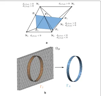
the cutting plane, and a corresponding base pointPon the plane given by one of the inter-section points. The concept is visualized in Fig.8. Note, that in the proposed approach the set of four signed nodal distance values is computed in a purely local operation. Hence, each background element has its own set of nodal distances. Therefore, in the following, this set of distances is referred to as elemental distances. These elemental distances finally define the discontinuous (element-wise) distance function. Having defined the discon-tinuous distance function, an approximation of the immersed structure appears as zero isosurface within the background mesh.
Visualization of the approximated immersed geometry
inter-sected at four points, the corresponding quadrilateral area is recreated as two neighboring triangles with similar orientation. All triangles are finally collected in a container and may be visualized as a common surface mesh.
The procedure is conceptually visualized in Fig.9a. In the figure, two distance valuesdi
anddjare computed for every edge in each tetrahedron separately. These values describe
the distances of the two corresponding edge nodesNiandNjto the immersed boundary.
If the product of both distance values is positive, then the corresponding element is not intersected by an immersed geometry. In case the product is negative, however, it means that the tetrahedron is intersected at this edge and the corresponding intersection point
Pcan be computed by linear interpolation:
P= | |dj|
di| + |dj|·Ni+ |di| |di| + |dj|·Nj
. (2)
In the given example, the distance values indicate that both tetrahedrons are intersected, whereas the linear interpolation results in one element with four intersection points and one with three intersection points. Correspondingly, three triangles can be reconstructed. These three triangles eventually represent a local reconstruction of the immersed bound-ary as it is seen by the two tetrahedrons (the background mesh).
A more complicated example is given in Fig.9b, where the implicit representation of an immersed cylinder is visualized. It is important to realize that the resulting triangular surface mesh (A) is different from the original immersed surface mesh (I given as
STL) and only serves visualization purposes. Thus, the supposedly bad quality of the reconstructed surface mesh (see the blue mesh in Fig.9b) is only a result of the chosen visualization technique and does not have any further implications. This is important to remember in the follow-up sections, when results of a surface approximation are shown with feature lines for a better distinction of individual geometrical aspects.
Determination of cutting planes for different intersection patterns
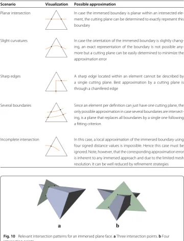
As explained in “Computation of elemental distances” section, in order to implicitly describe an immersed object, its boundary is approximated by a collection of planar cutting planes defined for each intersected element of the background mesh. Therefore, this cutting plane has to be determined depending on the local intersection pattern. Deter-mining this pattern is a challenging operation since different geometries may locally result in the same intersection pattern. Because of that, no unique definition of the cutting plane is possible. Thus, numerous special cases have to be considered in order to obtain a robust algorithm. How to determine the cutting plane for the most important scenarios is dis-cussed in this section. All of these scenarios and the corresponding intersection patterns are conceptually visualized in Table1. Note, that the scenarios are visualized in 2D but they are readily transferable to the three-dimensional case.
Approximation of planar surfaces
a
b
Fig. 9 Visualization of the geometry approximation resulting from an implicit description of the immersed object by a discontinuous distance function.aConcept: visualization by surface reconstruction.bExample: approximation of an immersed cylinder
cutting plane is defined using three of the possibly four given intersection points together with the surface normal vector from the immersed boundary.
To evaluate the corresponding approximation quality, the algorithm is tested for the case of a simple triangulated plate immersed into a box-shaped background mesh with around 19,000 elements, see Fig.11a. The testing process is as follows: first, the elemental distances are computed as described in “Computation of elemental distances” section, whereas immersed planar surfaces are treated as introduced above. Then, the hereby approximated surface is reconstructed and visualized following the approach introduced in “Visualization of the approximated immersed geometry” section. The resulting approx-imation of the immersed structure is presented in Fig.11b.
Table 1 Scenarios of immersed geometries leading to different intersection
patterns—the geometric complexity increases from the top to the bottom of the table
Scenario Visualization Possible approximation
Planar intersection In case the immersed boundary is planar within an intersected ele-ment, the cutting plane can be determined to exactly represent this boundary
Slight curvatures In case the orientation of the immersed boundary is slightly chang-ing, an exact representation of the boundary is not possible any-more but a cutting plane can be easily determined to minimize the approximation error
Sharp edges A sharp edge located within an element cannot be described by a single cutting plane. Best approximation by a cutting plane is through a chamfered edge
Several boundaries Since an element per definition can just have one cutting plane, the only possible approximation in case several boundaries are intersect-ing, is a plane that replaces all boundaries by a single one following a fitting criterion
Incomplete intersection In this case, a local approximation of the immersed boundary using four signed distance values is impossible. Hence this case must be ignored. Note, however, that the corresponding approximation error is inherent to any immersed approach and due to the limited mesh resolution. It can be well reduced by refinement strategies
Fig. 10 Relevant intersection patterns for an immersed plane face.aThree intersection points.bFour intersection points
Approximation of curved surfaces
As opposed to planar geometries, a curved surface generally can not be approximated exactly by a single cutting plane since the normal vector of the immersed boundary changes its direction within the intersected element. Therefore, a decision has to be made in terms of a normal vector and a base point in order to describe a plane which best approximates the immersed boundary. To this end three different cases are considered:
Fig. 11 Test case to evaluate surface approximation for immersed planar geometries.aTest setup: plate immersed into box-shaped background mesh with∼19,000 elements.bReconstruction of the immersed boundary (A)
Fig. 12 Concept to approximate a slightly curved immersed boundary within a background element
Given an intersection pattern with three intersection points (P1,P2,P3), a good approx-imation of the immersed boundary is easily obtained by the triangle formed from these intersection points. Therefore, the cutting plane is defined to be this triangle, whereas one of the intersection points is chosen as base point of the plane and the normal vector is derived from the cross product of two edges:
n= −−→P1P2× −−→P1P3. (3)
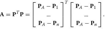
Case: four intersection pointsIn the case of four intersection nodes, the points are generally not located in a common plane anymore. In this case, a best-fit approach is chosen to compute the cutting plane such that it has a minimal distance to all intersection points. To formulate the corresponding optimization problem, first recall the equations which define the four nodal distancesdiof the corresponding background element:
d1= n
n·(PA−P1), (4a)
d2= n
n·(PA−P2), (4b)
d3= n
n·(PA−P3), (4c)
d4= n
Here,ndefines the unknown normal of the approximation plane. PA defines a base
point on the plane and Pi represents the position of thei−thintersection point. The
above equation can be rewritten in matrix form as follows:
d= n
nP, (5)
whereas the matrixPcollects the distance vectors between the intersection points and the base point of the plane:
P= ⎡ ⎢ ⎢ ⎢ ⎣
PA−P1
PA−P2
PA−P3
PA−P4 ⎤ ⎥ ⎥ ⎥
⎦. (6)
To find an optimal compromise for the cutting plane, a least squares approximation is applied, and the unknown normal vector as well as the unknown base point are chosen such that the nodal distances are minimized:
minimize n,PA
f : f = d2= 1
n2 ·n
T
PTP
A
n. (7)
In the last equation the matrix productPTPis summarized to a matrixA. To reduce the
problem, the base point is predefined as average point over all given intersection points:
PA=
1 4
4
i=1
Pi, . (8)
Furthermore, a unit surface normal is required, such that:
nTn=1. (9)
The final formulation of the least-squares problem reads:
minimize
n n
T
An
subject to nTn−1=0.
(10)
This corresponds to a constrained quadratic optimization problem. To solve for the three unknown components of the normal vectorn= {nx, ny, nz}, a Lagrange functionL
is formulated using the Lagrangian multiplierλ:
L(n,λ)=nTAn+λ(nTn−1). (11)
The stationary point ofLis obtained based on the following necessary conditions:
∂L
∂n =An+λn=0 (12a)
∂L
Fig. 13 Special intersection pattern for curved geometries in which edges of the background mesh are intersected twice.a3D example.bClose-up of the same example
The first Eq. (12a), can be rearranged such that the following eigenvalue problem is obtained:
An=λn. (13)
Here,λdenotes the eigenvalue of the matrixAandnthe corresponding eigenvector. With this knowledge in mind, Eq. (13) is multiplied bynT, which results in:
nTAn=λ. (14)
As the left hand side in this equation now characterizes the objective functionf [refer to Eq. (7)], one can deduce from (14) that the objective value is minimal ifncorresponds the eigenvector of the symmetric matrixAwith the smallest eigenvalue. Hence the normal which best fits the cutting plane to the four intersection points is chosen to be this eigen-vector. The corresponding eigenvalue problem is solved using the iterative Gauss-Seidel method.
Case: double-intersected edgesAnother special intersection pattern which has to be consid-ered with immersed geometries having a curved surface, is the case of double-intersected edges. Such an intersection pattern is shown in Fig.13. In the figure, a curved geometry (blue) immersed in a non-visible background mesh intersects a selected tetrahedron from the background mesh (green) in six points, whereas the top edge of the tetrahedron is intersected twice. The situation is conceptually sketched in Fig.14a.
a b
Fig. 14 Approximation strategy for immersed geometries that are slightly curved and lead to
double-intersected edges.aConceptual illustration of the problem.bConceptual illustration of the solution strategy
is defined through a base pointPA, which averages allnintersection points:
PA=
1 n
n
i=1
Pi, (15)
and a surface normaln, which corresponds to the eigenvector associated to the smallest eigenvalue of the following matrixA:
A=PTP=
⎡ ⎢ ⎣
PA−P1 ...
PA−Pn
⎤ ⎥ ⎦ T⎡ ⎢ ⎣
PA−P1 ...
PA−Pn
⎤ ⎥
⎦. (16)
The solution strategy to determine a cutting plane for immersed geometries which are slightly curved or which lead to double-intersected edges is conceptually illustrated in Fig. 14b.
Having presented strategies to approximate the cutting plane in case curved geometries are immersed into a background mesh, the resulting approximation quality shall be inves-tigated in the following. Test example is a sphere positioned into a box-shaped background mesh. The background mesh corresponds to the one which was already used for the pla-nar test case shown in Fig. 11a. By construction, the sphere intersects the background mesh such that all of the above cases appear (i.e., there are background elements with three and four intersection points, and there are elements with double-intersected edges). The testing process is as follows: first the elemental distances are computed as described in “Computation of elemental distances” section, whereas curved surfaces are treated as introduced above. Then, the hereby approximated surface is reconstructed and visual-ized following the approach introduced in “Visualization of the approximated immersed geometry” section. The resulting approximation of the immersed sphere is presented in Fig.15a, b for two different resolutions of the background mesh.
Fig. 15 Surface approximation of a sphere immersed into a background mesh.aReconstruction of immersed boundary (A) given a coarse background mesh.bReconstruction ofAgiven a fine background mesh.cReconstruction ofAwithout considering double-intersected edges
a b
Fig. 16 Conceptual illustration of intersection patterns with sharp edges inside single background elements.
aCase: intersection points uniquely define a plane.bCase: approximation by a plane requires fitting
to a locally unsuccessful approximation of the cutting plane (see Fig.15c). From the pre-vious results, one can conclude, that the presented algorithm is able to handle immersed geometries with slight curvatures.
Approximation of surfaces with sharp edges
The description of sharp edges within single background elements is generally not pos-sible since in the present approach only one cutting plane can be defined per element. However, this situation appears frequently unless the immersed geometry is completely smooth. Hence a proper approximation of sharp edges has to be found. To find such an approximation, two different intersection patterns shall be distinguished. Both patterns are conceptually illustrated in Fig.16.
a b
Fig. 17 Strategies to approximate sharp edges within single background elements.aCase: intersection points uniquely define a plane.bCase: approximation by a plane requires fitting
Fig. 18 Surface approximation of a cube immersed into a coarse background mesh to demonstrate the implicit description of sharp edges (feature lines are hidden)
as already described in “Approximation of curved surfaces” section, is followed in this case. The two solution strategies are conceptually illustrated in Fig.17.
Having presented strategies to approximate sharp edges within single background ele-ments, the resulting approximation quality shall be investigated in the following. Test example is a cube positioned into a box-shaped background mesh. The background mesh corresponds to the one which was already used for the planar test case shown in Fig.11a. The testing process is as follows: First the elemental distances are computed as described in “Computation of elemental distances” section, whereas sharp edges and planar sur-faces are treated as introduced above and in “Approximation of planar sursur-faces” section. Then, the hereby approximated surface is reconstructed and visualized following the approach introduced in “Visualization of the approximated immersed geometry section”. The resulting approximation of the immersed cube is presented in Fig.18.
a b
Fig. 19 Improper / misaligned approximation of cutting plane in case several boundaries are intersecting a single background element.aSeveral boundaries intersecting a single element.bWrong approximation of cutting plane following a best-fit approach
Approximation in case several boundaries are intersecting
Since a specific background element can per definition just have one cutting plane, the only possible approximation, in case of several intersecting boundaries, is a plane. This plane replaces all boundaries by a single one and is determined following a fitting criterion. In doing so, it must be accepted that all information about the single boundaries is lost. This loss of information, however, is not necessarily a bad characteristic. As a matter of fact, it allows to properly describe immersed geometries even if they are badly modeled and contain overlaps or duplicated geometries. More precisely, when several boundaries within one intersected background element are replaced by a single one, overlaps or dupli-cated geometries are simply “overseen” and therefore do not cause any further problems. i.e., a robust treatment of such “dirty geometries” is an inherent property of the pre-sented approach. The specific strategy to approximate several immersed boundaries by one cutting plane is described in the following:
Consider the conceptual illustration of the problem in Fig.19a. The figure visualizes a case where two distinct immersed boundaries are traversing the same elements of the background mesh. The corresponding intersection pattern is characterized by the fact that there are more than three intersection points and double-intersected edges. Therefore, an obvious way to approximate the immersed boundary by a cutting plane would be again a best-fit approach, much like it was already proposed in the previous sections for similar intersection patterns. However, if one actually approximates the immersed boundaries by a single plane determined through a best-fit procedure, it is possible to obtain an approximation of the geometry as depicted in Fig.19b. As can be seen from the figure, the best-fit approach may result in an approximated cutting plane which indeed is “optimally” placed between the intersection points, but its orientation is clearly wrong. Instead, one would expect the cutting planes to be aligned with the two opposite surfaces.
Fig. 20 Approximation of a properly aligned cutting plane for the case of multiple boundaries crossing single background elements
a
b
Fig. 21 Problematic intersection pattern with the approximation of a wing in a background mesh.aWing model.bElement with several immersed boundaries at the sharp edge of the wing
n= 1
m
m
i=1
ni, (17)
To avoid cancellation in case individual surface normals point in opposite directions, meaning their enclosed angle exceeds 90◦, all vectors are firstly aligned to the first in the sum. I.e., iffni·n1<0, thenni = −ni. The final approach is illustrated in Fig.20.
As already mentioned above, such a solution for the approximation of several immersed boundaries by a single cutting plane is advantageous if immersed objects contain modeling errors. However, it also plays an important role in cases where thin or tapered structures are immersed into a background mesh. As an example, consider the wing shown in Fig. 21a. Putting this wing into an arbitrary tetrahedral background mesh, there will be most likely a lot of elements around the sharp edge, which are intersected by several immersed boundaries (see Fig.21b). Therefore, a proper treatment of these cases is decisive for the overall approximation quality. The achievable approximation quality for the presented wing is discussed in “Refinement strategies to improve the approximation quality” section in the context of mesh refinement.
Summarized strategy to determine local cutting planes
Fig. 22 Strategy to determine the cutting plane for a given intersected background element. Determination requires a base pointPAand a normal vectorn.Pidenotes the intersection points
which was chosen in the individual case, was depending on the number of intersection points as well as the local intersection pattern. Figure22summarizes the proposed overall strategy to determine the cutting plane for a given intersected background element.
Refinement strategies to improve the approximation quality
In the context of immersed methods, the size of the elements in the background mesh generally defines a length scale up to which geometric details of the immersed object can be resolved. Consequently every detail smaller than this length scale is simply neglected. The approximation quality is hence directly depending on the resolution of the background mesh and, if necessary, may be controlled by means of refinement strategies. Note that the dependency of the approximation quality on the resolution of the background mesh may be actually seen as a very beneficial characteristic since it inherently allows to handle flaws in the description of the immersed geometry (like gaps, overlaps, etc.) and it allows to exploit a multiresolution analysis in the case of complex investigation scenarios.
In case the approximation quality must be improved, an adaptive mesh refinement in two steps is proposed: first, in a loop over all elements of the background mesh, ele-ments that satisfy a specified refinement criterion are tagged. Then, in a second loop over the elements, all tagged elements are refined using the algorithm described in [19]. As refinement criterion, the local approximation quality is utilized, i.e., only those elements shall be tagged, which cause problems in the approximation of the immersed geometry. Within this paper, three of such problematic cases are considered. They are conceptually summarized in Fig.23.
The first problematic case is identified when an element of the background mesh is intersected by the immersed geometry such, that it contains an edge which is cut twice (see Fig.23a). In order to properly approximate the immersed geometry in this case, the corresponding element has to be refined until the two opposite surfaces fall into different elements of the background mesh.
a b c
Fig. 23 Problematic cases to be tagged for refinement.aDouble-intersected edges.bHigh change in curvature.cElements with no cutting plane
slightly curved or even planar, the change of normal vectors is small, i.e., no refinement is necessary. But if the curvature is large or the object changes its direction within an element, the element needs to be refined. Therefore, in case the normal orientation of the immersed geometry changes within a single background element, every pair of surface normals at the intersection points,n1andn2, is compared. If the corresponding angular change exceeds an adjustable limit ofα, the element is also tagged for refinement.
As third and last indicator, consider the case in which a background element is just slightly touched by the immersed object such that no cutting plane can be approximated (e.g., only one edge of the element is cut, see Fig.23c). As pointed out earlier in “Geometri-cal representation of immersed objects using a discontinuous distance function” section, elements where no cutting plane can be approximated are simply ignored. As this will obvi-ously introduce an error in the approximation of the immersed geometry, a refinement shall be triggered here. Note, that unlike in the previous two cases, a refinement will in this case not completely cure the problem as there will be always one element at the very edge of the immersed geometry. But by refinement, this problem may be reduced to a negligible influence. The final adaptive mesh refinement algorithm in pseudocode reads as follows:
//1 Tag problematic elements to be refined
forElementinBackgroundMeshdo
DetermineCuttingPattern()
ifncut_edges<3orndouble_intersected_edges>0or (n1,n2)> αthen: TagElement()
end if end for
// 2. Refine all tagged elements
forElementinBackgroundMeshdo
ifElement.IsTagged()then: RefineElement()
end if end for
Fig. 24 Model setup to test the proposed refinement strategy with regard to possible improvements in the approximation of immersed objects.aOverall model setup with wing placed into a background mesh.b
Section view through the background mesh around the wing for a size comparison
mesh is large compared to the characteristic dimensions of the immersed object. For a size comparison, refer to Fig.24, which shows the overall setup as well as a section view around the wing.
The resulting approximation of the wing without any refinement of the background mesh and following the procedure discussed in “Geometrical representation of immersed objects using a discontinuous distance function” section is presented in Fig.25a. As can be seen, without any refinement, the surface of the wing is quite porous and the leading and the trailing edge is not well approximated. However, already after applying one refinement iteration (α=30◦), the results can be improved significantly, as shown in Fig.25b. Further refining the background mesh finally results in a continuously better resolved geometry, see Fig.25c, d. After five levels of refinement already a very good surface quality is obtained. With regard to the background mesh, the number of elements hardly increases after the first three levels of refinement. This is because additional elements are only introduced around critical areas, i.e., mostly along the edges and regions with a low geometry reso-lution. This quickly fixes large surfaces and repairs comparably slower the edges. Only if one wants to further resolve geometric details, such as the sharp edges here, more levels of refinement are necessary. In the present case this leads to 2.2e6 elements after five repetitions of the proposed refinement strategy.
Fig. 25 Approximation of an immersed wing geometry within a background mesh after different levels of refinement.aNo refinement (4.0e5 elements).b1 level of refinement (4.4e5 elements).c3 levels of refinement (6.2e5 elements).d5 levels of refinement (2.2e6 elements)
Fig. 26 Approximation of a cube immersed into a refined background mesh.aSection view of the refined background mesh with immersed cube (nodes of the entire background mesh are highlighted).bResulting surface approximation within the refined background mesh
accumu-102 103 104 105 106 107 number of background elements
10-4 10-3 10-2 10-1 error adaptive refinement
102 103 104 105 106 107
number of background elements
10-4 10-3 10-2
10-1 uniform refinement
102 103 104 105 106 107
number of background elements 10-4 10-3 10-2 10-1 error uniform refinement
Fig. 27 Quantitative study of the approximation error for a sphere immersed into a continuously refined background mesh (The dots indicate six levels of refinement following two different strategies)
lation around the edges is due to the additional elements, which were introduced into the background mesh during the refinement.
After the previous focus on qualitative aspects, a quantitative evaluation of the geometric approximation quality is presented in the following. As a precisely defined test case, a sphere with the radiusr= 0.4 is positioned into a box-shaped background mesh, which then is refined several times, both uniformly at every intersection and adaptively using the above presented algorithm withα = 1◦(i.e., if the surface normal of the immersed geometry within a single intersected background element changes by more than one degree, the corresponding element is refined). For every mesh, the following error measure is evaluated:
= ||r−r˜i||max (18)
In this equation, ˜rirepresents the approximated radius at thei-th node of the
approxi-mated sphere, and|| · ||maxthe maximum norm. Figure27summarizes the results of this
study.
locally result in problematic elements again, which explains the sudden error increase in the last iteration of the uniform strategy.
From all the previous results in this section, it can be concluded, that the proposed com-bination of adaptive mesh refinement and implicit geometry description results in high quality surface approximations with a manageable number of elements in the background mesh.
Identification of closed regions using a continuous distance function
For the special case that closed geometries shall be described implicitly within a given background mesh, an algorithm is presented in the following, which allows to distinguish regions inside the closed domain from regions outside of it. The approach relies on a continuous distance function which is formulated based on the discontinuous distance function presented in “Geometrical representation of immersed objects using a discon-tinuous distance function” section. The condiscon-tinuous distance function is constructed such that it assigns each node of the background mesh a unique negative distance value if it lies inside the immersed geometry, and a unique positive distance value else. The proposed algorithm consists of the following three basic steps:
1. Calculate elemental distances: Calculate for each intersected element separately the nodal distances following the above introduced discontinuous distance calculation. 2. Determine absolute nodal distances: Determine for each node of the background
mesh a unique distance value by finding the smallest distance value associated to this node in all intersected neighbor elements.
3. Determine signs: Determine for each node if it lies inside or outside the closed region using a specially tailored ray casting algorithm.
The first step recalls the techniques introduced in “Geometrical representation of immersed objects using a discontinuous distance function” section and the second step corresponds to a straightforward operation. Thus, in the following, the focus is on the last step. In this last step, it has to be determined whether a given node lies inside or outside the closed geometry. This operation is known in literature as the point-in-polygon (PIP) problem [35–37].
There are several algorithms to solve the PIP problem. Many of them rely on watertight boundaries or a proper orientation of surface normals. However, in case of complicated geometries or models from practice, none of these two characteristics can be guaranteed. Correspondingly, an approach is proposed in the following, which does not utilize such information. Instead, an algorithm based on ray casting is elaborated. Note, that a common alternative to this ray casting would be an approach based on voxelization, see e.g. [38,39]. However, such an algorithm strongly depends on the voxel size for non-clean geometries, which is why this alternative was avoided.
Basic ray casting
Fig. 28 Concept of ray casting to identify inside and outside of a closed geometry: Start from outside and determine the status of a given node by following the status of the ray, which changes after each intersection with the boundaries
existing methods, a classical approach is the ray intersection method [35]. In this method, a random ray is emitted from the point of interest and the resulting number of intersections between this ray and the surface contours of the given 3D object is counted. If the number is even, the point is outside the 3D object. If it is odd, the point is considered inside. A slightly modified version of this method is used within the current work to solve the problem of assigning signs to the nodal distance values. The modifications are mainly introduced to increase the algorithm’s robustness in case of deficient (“dirty”) geometries. One modification is the following: Instead of starting from the point of interest, the ray is always shot from a point outside of the domain to a node of interest within the background mesh, and from there to a point outside again. In doing so, the ray is aligned to the Cartesian directions. The latter improves the efficiency of the intersection search and the fact that it starts and ends outside may be later used for the purpose of ray validation. Given such a ray, all intersections between the immersed geometry and the ray are determined, whereas in direction of the ray, every intersection causes a change of its status (inside or outside the immersed geometry). That is, starting from a point outside, the first intersection indicates that the ray entered the inside of the immersed geometry. Another intersection then indicates that the ray is outside again, and so forth. The position of the actual node of interest is then determined by the current status of the crossing ray. Finally, a positive sign is assigned to the node’s distance value if the ray indicates a region outside and a negative value else. A 2D example of the approach is illustrated in Fig.28. Further modifications of the ray casting algorithm are discussed in the following sections.
Improvements for non-watertight geometries
The ray casting technique has a deterministic behavior for clean geometries so that one ray is enough to univocally determine whether a node is inside or outside. However, for non-watertight geometries there are many possibilities for which the basic technique fails. Considering the non-watertight geometry with gaps and overlaps depicted in Fig.29, the failure cases are:
Fig. 29 A non-watertight geometry with gaps and overlaps
Fig. 30 Errors in the modeled geometry, which lead to an erroneous coloring (wrong identification of inside / outside status).aSituation with gaps.bSituation with overlaps
2. The ray passes through an overlapped part (see Fig.30b). In this situation, the ray would detect two intersection points when entering the geometry leading to the wrong conclusion that after the second intersection it is again outside.
To deal with these problems, it proposed to use several rays for a specific node of interest, i.e., one ray for every coordinate direction, and decide on the nodes position by voting. The concept is adopted from an approach to simplify and repair polygonal models [41]. In the three-dimensional case for example, if one ray passes through a gap or overlapped region, the other two rays would vote for a correct result. Hence the node’s position can be determined correctly. Figure31conceptually illustrates the approach for the two-dimensional case with two rays. From the experience of the authors, this simple idea works well in practice and can handle the majority of modeling errors by the cost of an increased ray casting time. However, the latter is negligible compared to the rest of the algorithm presented in this paper.
While the proposed mechanism of voting works well in practice, there is still the lit-tle possibility that two or even all rays are passing conflicting areas leading to wrong conclusions. To this end several improvements are included:
Fig. 31 Concept of voting: two rays vote whether a certain node is inside or outside. Then a decision is made based on the votes. Here, one ray is voting for outside and the other for inside. Note that in 3D, there is one more ray, so that a draw is not possible
Fig. 32 Improvements for on increased robustness of the ray casting algorithm.aExclusion of an invalid ray from voting.bLocal ray casting
exclusion of an invalid ray prevents false conclusions with respect to a node position is given in Fig.32a.
2. Collapse adjacent hits: If a ray detects two intersections that are very close (in com-parison with the element size), they are collapsed in order to better deal with overlaps. 3. Local ray casting: Invalidating rays may result in situations where all rays are con-sidered invalid or where two valid ones give different results. In such cases, a local ray casting from neighbor nodes with known color (inside/outside status) will be performed. Therefore, local rays are sent from these neighbors to the one node to be colored. Then the final color is decided by voting again. The concept is illustrated in Fig.32b.
It should be remarked, that the concept of voting and all the other above improvements do not reduce the theoretical possibility of failure to zero. But in practice, they yield a very robust algorithm to determine the sign of all distance values respectively all inside and outside areas.
Cases that include double-sided geometries
deter-Fig. 33 Combination of closed (solid line) and double-sided structures (dashed line): double-sided structure is marked by a flag and then simply ignored in the ray casting algorithm
mine inside or outside areas since the ray will also count hits with the double-sided object. To this end, a previous mark-up is introduced. That is, in cases where both, double-sided geometries and closed volume bodies are immersed into the same background mesh, the double-sided geometries are flagged prior to the ray casting. Hits with flagged geometries will then simply be neglected in the actual ray casting afterwards. Hence inside and outside areas may again be properly defined. The concept is illustrated in Fig.33.
Examples of immersed geometries with different features and challenges In this chapter, the implicit description of geometry within a background mesh using the above presented strategy is tested for several geometries with varying complexity. The goal is to demonstrate its capabilities and its applicability in conjunction with complex 3D geometries. Therefore, three test cases from different fields of application are considered. The first one is a sail model representing the general case of a surface geometry immersed into a computational background mesh. The second case represents a section model of an inflatable hangar with which the situation for closed volume geometries shall be investigated. The last test case comprises a complete racing car and hence combines all the aforementioned cases to a complex problem, as it has to be expected for industrial examples.
The testing procedure is as follows: first, the geometry under consideration is placed into a simple block-shaped domain which is meshed with equally distributed tetrahedral elements as it may be obtained from any meshing software within a short period of time. Then, the complete algorithm, as presented in this paper and as outlined in Fig. 4, is applied to implicitly describe the immersed geometry with respect to the given background mesh. Finally, the implicit description of the geometry is used to reconstruct a surface approximation (see “Visualization of the approximated immersed geometry” section), which in a last step is then compared to the original model. Note, that in the following, a visualization of the background mesh is omitted to avoid clutter.
Surface geometries
Fig. 34 STL model of sails to be represented within a background mesh
background mesh, whereas the particular focus is on how well the curved surface areas and free edges are approximated.
Applying the presented algorithm to implicitly describe the sails within the given back-ground mesh, the surface approximation presented in Fig.35a is obtained. From the latter one can see, that the curved surface regions are approximated very well such that the three different sails clearly form out without any unexpected approximation errors. At the free edges or sharp corners, however, there are striking defects that do not resolve the actual edge sufficiently. As a matter of fact, these defects arise from the special inter-section patters between geometry and background mesh at the free edges and can be considered as a problem of mesh refinement. Applying adaptive refinement as introduced in “Refinement strategies to improve the approximation quality” section, the quality of the approximation can be significantly improved up to a point where the free edges are accurately captured, see Fig.35b. It is worthwhile to mention, that this test case includes a point where different geometric entities (two sails) touch each other such that a G0-continuous connection forms out. As can be seen from Fig.35b, also the area in the direct vicinity of this connection point is accurately resolved, which can be traced back to the advantages of the discrete distance function that identifies the immersed boundary in a purely local operation.
Closed volume geometries
Fig. 35 Reconstructed surface approximation of sails immersed into a block-shaped background mesh.a
Without adaptive refinement of background mesh (∼800,000 elements).bWith four levels of adaptive refinement (ca. 4.5 Mio. elements)
Applying the presented algorithm to implicitly describe the hangar section within a background mesh of initially 800,000 tetrahedrons, the surface approximation presented in Fig.36b is obtained. Even though the tubes and surface regions are clearly forming out as expected, there are striking defects around the sharp edges on the ground. Similarly as in the previous section, this is mostly because of the low resolution of the background mesh, which yields very difficult intersection patterns for areas with rapidly changing geometric characteristics such as the sharp edges. The defects can be resolved by an adaptive refinement of the background mesh, see Fig. 36c. Moreover, the refinement leads to a proper capturing of the hangar’s closed regions, see Fig.36d.
Apart from the pure approximation of the immersed geometry, also inside and out-side regions were identified following the approach described in “Identification of closed regions using a continuous distance function” section. Figure37shows the corresponding results for an arbitrary cross-section of the hangar. From the figure it may be seen, that only the nodes inside the geometric boundaries, so the nodes that are part of the pressur-ized volume, are tagged with a negative signed distance, whereas all the others obtain a positive sign. The signs allow for a clear distinction of the different parts in the computa-tional mesh. The corresponding information may for example be utilized in an immersed CFD simulation where the interior and the exterior flow need to be treated differently. It is worthwhile to mention, that this distinction was performed without referring to the surface normals of the geometry. By doing so, any problems related to misaligned nor-mals, as they often occur in practical applications, are avoided. From the previous results it is evident, that a combination of discontinuous and continuous distance function, as proposed in this paper, can be utilized effectively to represent closed geometries within a background mesh.
Combined arbitrarily complex geometries
Having tested both, closed and double-sided geometries individually, the presented algo-rithm is in this section applied to a large-scale example, which includes both cases. The model under consideration represents a complete racing car and contains rather sim-ple as well as very comsim-plex geometric features on various length-scales ranging from large-spanned surface areas to detailed geometric objects. The corresponding geometry is depicted in Fig.38. As a reference discretization, again a block-shaped tetrahedral mesh is used, whereas this time, the initial discretization is intentionally chosen to be very coarse (only 40,000 elements). Starting from that coarse discretization, the background mesh is gradually refined, and in each case the corresponding implicit surface representation is evaluated.
Fig. 37 Sign of nodal distances at a cross-section of the hangar (a positive sign indicates a node outside the tubes and a negative sign a node inside).aPosition of cross-section.bSign of nodal distance values
Fig. 38 STL model of a racing car representing a complex geometry including surface and volume areas at different length-scales
in all its details within the background mesh, see Fig.39b, c. The resulting number of elements (1.6·106) thereby remains in an acceptable range. Particularly interesting to see is, that hollow regions at the air ducts and the driver cabin as well as the flat spoiler and undertray parts are generally detected and resolved.
Fig. 39 Surface approximation of racing car with different refinements of the background mesh.aNo refinement (4.0e4 fluid elements).b2 levels of refinement (9.5e4 fluid elements).c5 levels of refinement (1.6e6 fluid elements).dClose-up after last refinement
the immersed geometry). As a result an accumulation of feature lines or reconstructed elements indicates indirectly regions where the adaptive refinement actually refined the background mesh. Knowing the meaning of the feature lines, one can conclude from Fig. 39c, that spots on the race car with a complex geometry and difficult intersection patterns (spoiler, undertray, edges) are refined much more than wide surface areas or planar parts. This has to be expected from the adaptive refinement strategy.
Despite all the refinement so far, there are still local approximation errors on a small scale, mostly around edges (see close-up in Fig.39d). These local approximation errors still appear because the model contains very small details compared to its overall dimensions, i.e., the resolution of the background mesh is locally still too coarse. In fact, these errors can not be avoided completely, however, by further refinement of the background mesh, they may be reduced down to a scale where their impact is acceptable. In this context, Fig. 40shows the best surface approximation, which was obtained for the racing car within the present work.
Conclusion