R E S E A R C H A R T I C L E
Open Access
Toward 4D mechanical correlation
François Hild
1*, Amine Bouterf
1, Ludovic Chamoin
1, Hugo Leclerc
1, Florent Mathieu
1,
Jan Neggers
1, Florent Pled
3, Zvonimir Tomiˇcevi´c
1,2and Stéphane Roux
1*Correspondence:
1LMT, ENS
Cachan/CNRS/Université Paris-Saclay, 61 Avenue du Président Wilson, Cachan, France Full list of author information is available at the end of the article
Abstract
Background: The goal of the present study is to illustrate the full integration of sensor and imaging data into numerical procedures for the purpose of identification of constitutive laws and their validation. The feasibility of such approaches is proven in the context of in situ tests monitored by tomography. The bridging tool consists of spatiotemporal (i.e., 4D) analyses with dedicated (integrated) correlation algorithms.
Methods: A tensile test on nodular graphite cast iron sample is performed within a lab tomograph. The reconstructed volumes are registered via integrated digital volume correlation (DVC) that incorporates a finite element modeling of the test, thereby performing a mechanical integration in 4D registration of a series of 3D images. In the present case a non-intrusive procedure is developed in which the 4D sensitivity fields are obtained with a commercial finite element code, allowing for a large versatility in meshing and incorporation of complex constitutive laws. Convergence studies can thus be performed in which the quality of the discretization is controlled both for the simulation and the registration.
Results: Incremental DVC analyses are carried out with the scans acquired during the in situ mechanical test. For DVC, the mesh size results from a compromise between measurement uncertainties and its spatial resolution. Conversely, a numerically good mesh may reveal too fine for the considered material microstructure. With the
integrated framework proposed herein, 4D registrations can be performed and missing boundary conditions of the reference state as well as mechanical parameters of an elastoplastic constitutive law are determined in fair condition both for DVC and simulation.
Keywords: Digital volume correlation, Identification, Integrated approaches, Tomography, Verification
Background
The emergence of simulation-based engineering sciences calls, among many chal-lenges [1], for robust validation procedures and uncertainty quantifications to achieve reliable predictions. Full-field measurements are one way of bridging experimental and computational mechanics. Their advantage lies in the fact that the comparison is now achieved by using huge amounts of data, including 3D imaging, to probe the predictive capacity of material models [2] and numerical frameworks [3]. The aim of the paper is to show that a seamless procedure, hereafter called “integrated 4D registration,” can be formulated to analyze an in-situ test performed in a lab tomograph for the purpose of identifying a nonlinear constitutive law and unknown boundary conditions.
©The Author(s) 2016. This article is distributed under the terms of the Creative Commons Attribution 4.0 International License (http://creativecommons.org/licenses/by/4.0/), which permits unrestricted use, distribution, and reproduction in any medium, provided you give appropriate credit to the original author(s) and the source, provide a link to the Creative Commons license, and indicate if changes were made.
Computed microtomography allows 3D images of materials to be obtained, which reveal the microstructure in the bulk in a non-destructive way [4–8]. Very early on, mechanical tests were performed in-situ [9–12]. For instance, the damage development in particulate composites could be analyzed [11,13,14]. Creep has also been studied with such tech-niques [15–18]. One additional feature is to quantify kinematic fields via digital volume correlation (or DVC [19,20]). This additional piece of information can be used to ana-lyze fatigue crack propagation [21,22] or to validate finite element simulations of cracked samples [3].
Very few studies deal with the identification of material parameters based on volumetric analyses. A first reason is related to the measurement uncertainties and biases that are usu-ally higher than those typicusu-ally encountered in 2D analyses [23,24]. Second, the computa-tional environment needed to solve these inverse problems is generally very intrusive (e.g., constitutive equation gap method [25–27], virtual fields method for nonlinear constitutive laws [28], equilibrium gap method [29]). Third, nonlinear constitutive equations require spatiotemporal (i.e., 4D) analyses to be considered, which are both experimentally and computationally very demanding. The aim of the present work is to show the feasibility of such a framework to study the elastoplastic behavior of spheroidal graphite (SG) cast iron. One of the goals of the present study is to achieve full integration of sensor and measure-ment data in the developed numerical procedures [1]. This type of analysis corresponds to so-calledintegratedapproaches [30,31], which were developed up to now mostly with 2D images of sample surfaces [32–36] in which material parameters are directly measured from image registrations. A first extension to 3D images was recently proposed to analyze an indentation experiment on plasterboard monitored via tomography and DVC [37]. When material parameters are sought, the corresponding kinematic and static sensitivi-ties [38] are needed. Finite element simulations are used in particular to generate a set of kinematic fields that are further used for DVC purposes. It was shown that non-intrusive spatiotemporal schemes can be used for 2D images [39], whereby the incorporation of time leads to 3D integration. In a similar spirit but extended to 3D (spatial) images, the following analysis corresponds to a first step toward 4D integration.
In “Methods” section, the experimental configuration is presented. DVC analyses based upon discretizations with 4-noded tetrahedra (i.e., T4-DVC) are used to measure kine-matic fields without any mechanical regularization. From the acquired scan in the ref-erence configuration, a mesh is adapted to the actual shape of the sample. From the kinematic measurements, the measured nodal displacements of the top and bottom faces of the region of interest (ROI) become the boundary conditions of the integrated scheme in which the material parameters are sought. A non-intrusive setting is developed. The previous framework is applied to analyze the described tensile test on spheroidal graphite cast iron to determine unknown boundary conditions, and to identify elastoplastic para-meters (“Results and discussion” section). Uncertainty quantifications are performed in addition to convergence analyses in which the mesh quality is assessed as well.
Methods
In situ mechanical test
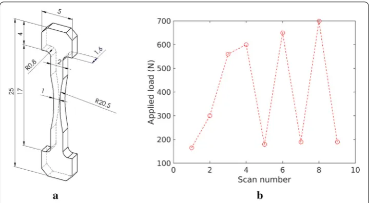
Fig. 1 In situ tensile test.aDog-bone sample used for tomography. The dimensions are expressed in mm. bLoading history for the in situ tensile test
area and not in the grips, the central part is thinned with a radius of 20 mm (Fig. 1a). This zone is 9-mm high, while the smallest cross-section of the sample is 1.6×1 mm2. The tensile test reported herein has been carried out in the X50+tomograph of LMT. The specimen is loaded in nine incremental loading and unloading steps (Fig. 1b) in a custom made testing machine, which is placed on the turntable of the tomograph [40]. It is worth noting that the reference scan is acquired at a load level equal to 165 N. The first two scans of the reference configuration allow displacement uncertainties to be evaluated.
A complete scan of the sample corresponds to a 360◦rotation along its vertical axis, dur-ing which 1000 radiographs are acquired with a definition of 1280×1860 pixels. Each scan lasted less than 40 min. The physical voxel size is 6.4µm, and the reconstructed volume is encoded with 8-bit deep gray levels. This test was analyzed via global approaches to DVC with regular meshes made of 8-noded cubes to reveal the damage micromechanism (i.e., nodule debonding) with the correlation residuals [41]. In the following, the underlying macroscopic behavior will be studied.
Digital volume correlation
DVC is used to measure 3D displacement fields in the bulk of samples [42,43]. In its incre-mental version, DVC consists of registering two volumes by evaluating displacement fields that yield the best possible match. In the early developments, small zones of interest or ZOIs (i.e., small interrogation volumes [19,20,44,45]) in the considered region of interest (ROI) are registered. This type of approach is nowadays referred to aslocal(i.e., the only information that is kept is the mean displacement assigned to each analyzed ZOI center) and incremental since only two volumes are considered. Each registration is performed over the ZOI with various kinematic hypotheses, possibly accounting for its warping. This type of analysis is not considered herein since it does not offer an interpretation of the kinematic measurement that is “congruent” with that of FE analyses.
formulations). The fact that continuity is enforced allows the measurement uncertainty to be reduced in comparison with the samediscretization in which the nodes are not shared [47]. Another important advantage of global DVC in comparison with local DVC is its direct link with numerical simulations of mechanical problems [3,21]. When dealing with digital volumes it is natural to consider regular meshes made of 8-noded cubes (i.e., C8-DVC [46]) even though unstructured meshes may also be considered [48]. In the following, unstructured meshes made of 4-noded tetrahedra are chosen to allow for a more faithful description of external surfaces (“Mesh of the ROI” section) in comparison with structured C8 meshes.
The incremental registration problem (i.e., digital volume correlation) consists in min-imizing the sum of squared differences
umeas=Argmin u
ROI
(I0(x)−It(x+u(x)))2
2γI2 (1)
over the considered ROI for the reconstructed volumes in the reference configurationI0(x)
and deformed configurationIt(x).γI2denotes the variance associated with acquisition and reconstruction noise of the gray level volumes. For the sake of simplicity and in line with the chosen formulation (1), the latter is assumed to be white and Gaussian. This is a rather crude assumption for computed tomography, for which as its very name indicates, the raw data (i.e., radiographs) are processed to provide the reconstructed volume [49], and thereby the original noise in the radiograph displays in the reconstructed volume a nonho-mogeneous character and exhibits strong and anisotropic spatial correlations. However, even if this assumption is not optimal, from previous experience, it revealed sufficient for handling DVC for standard tomographic images. Correlation residuals however do reveal systematically more pronounced levels close to the rotation axis and artifacts such as rings [23,50].
Equation (1) expresses the underlying assumption of gray level conservation for each considered voxelxof the ROI. This least squares problem is nonlinear. It is solved with an iterative Gauss–Newton scheme [51] in which the stationarity condition is recast in the following variational formulation [52].
Problem 1 Findδusuch thatA(δu,δv)=L(δv) for any incremental fieldδvwith A(δu,δv)= 1
2γI2
ROI
(δu· ∇∇∇I0)(x)(δv· ∇∇∇I0)(x) L(δv)= 1
2γI2
ROI
ρ(x)(δv· ∇∇∇I0)(x) (2)
and whereρ(x) = I0(x)−It(x+u(x)) is the current gray level residual,uthe current estimate of the sought displacement field,δuthe correction to the current displacement field, andδvan increment to the trial displacement field.
The subspace to which the measured and trial displacements belong is chosen to be the vector space generated by a set of fieldsϕn(x) so that
u(x)= n
where υn are the sought amplitudes at the considered time t (υn(0) = 0), which are gathered in the column vector{υ}. The minimization procedure consists of successive linearizations and corrections{δυ}to the measured degrees of freedom [53]
[M]{δυ} = {b} (4)
with
[M]=[]†[] and {b} =[]†{ρ} (5)
where{ρ}gathers all voxel-scale dimensionless residualsρ(x)/√2γI, and † denotes the transpose of a matrix or column vector. The DVC matrix [M] and the corresponding residual vector{b}are constructed with the matrix [] that gathers all scalar products of the basis fields by the volume contrast (i.e.,(x, n)=ϕn(x)·∇I0(x)/
√
2γI).
The covariance matrix [Covυ] of the measured degrees of freedom is given by [54]
[Covυ]=[M]−1 (6)
In the following analyses, 4-noded tetrahedra will be considered. Consequently the kinematic basis made ofϕn(x) fields corresponds to the shape functions of T4 elements. Such registration approach will be referred to as incremental T4-DVC.
Mesh of the ROI
To perform T4-DVC analyses, the ROI of the sample needs to be meshed based on its true geometry. This type of procedure usually requires the acquired scan to be processed with mathematical morphology and ad hoc procedures [55–57]. When multiphase microstruc-tures are studied, this operation becomes more complex to make sure that the mesh is compatible with the morphology of the phases. For instance, adaptive level-set method can be used [58]. In the present case, the simulations will not be performed at the microstruc-tural scale but using a macroscopic description of the material behavior. Consequently, the mesh will not be adapted to the underlying microstructure. However, it needs to comply with the external surface of the sample.
A digital image correlation procedure is implemented to adjust a regular mesh made of 4-noded quadrilaterals to the actual surface of the sample [59]. Different transverse sections are considered. From these registrations, a 3D discretization made of 8-noded hexahedra (H8) is obtained. It is subsequently converted into a T4 discretization by subdividing each H8 element into six T4 elements of equal volume. The two meshes are exactly node-equivalent, i.e., the number of nodes and the node positions are unchanged.
With a given discretization, one critical issue in DVC analyses is the measurement uncertainty. Because the registration is an inverse problem, it is expected that finer meshes will lead to poorer measurement uncertainties [47]. This effect can be understood by estimating the uncertainty associated with acquisition noise. Equation (6) shows that the covariance of measured degrees of freedom is related to the inverse of the DVC matrix. The latter is assembled by using elementary matrices [Me] of the T4 elements used in the mesh. The latter contains scalar products of the volume contrast (i.e.,∇I0(x)) and
the vector shape functions (i.e.,Ni(x)ep, withi = 1,4 andp= 1,3). Consequently, the components of sub-matrices [Mepq] read
(Mepq)ij = δpq 2γI2
VOIe
whereVOIecorresponds to the integration domain of the considered T4 element,Nithe (linear) shape functions of the T4 element, andδpqKronecker’s delta. If the correlation length of the gray level volume is smaller than a characteristic length scaleof the element a mean field approximation can be made [47]
(ep·∇I0)(eq·∇I0) ≈I2δpq (8)
whereI2=(1/3)∇I02is the mean square of the volume contrast. The expression of each sub-matrix then becomes
[Mepq]= δpq 2γI2
2 I3 20 × ⎡ ⎢ ⎢ ⎢ ⎣
2 1 1 1 1 2 1 1 1 1 2 1 1 1 1 2
⎤ ⎥ ⎥ ⎥
⎦ (9)
where 3 is equal to the volume of the T4 element and the corresponding covariance matrix
[Covepq]=δpq 8γ2
Iμ2
2 I3
× ⎡ ⎢ ⎢ ⎢ ⎣
4 −1 −1 −1
−1 4 −1 −1
−1 −1 4 −1
−1 −1 −1 4
⎤ ⎥ ⎥ ⎥
⎦ (10)
where μis the physical size of one voxel. The standard uncertainty for each degree of freedom reads
γυe= 4 √
2γIμ
I3/2
(11)
Equation (11) shows that the measurement uncertainty is related to the noise to signal ratioγI/I within the considered ROI, and is inversely proportional to the square root of the number of voxels within the considered T4 element. The standard displacement uncertainty γυe is two times lower than that of a regular hexahedron with thesame volume [47].
The elementary matrices [Me] are then assembled to evaluate the global DVC matrix [M] and the corresponding covariance matrix [Covυ]. In the assembly process, the nodal displacements will now be evaluated over more than one element (i.e., all the elements sharing the considered node). Consequently, the number of voxels3
gconsidered for the evaluation of the nodal displacements will become larger than that of each individual element. For a regular mesh made of C8 elements, the corresponding volume is equal to (2)3[47]. With the chosen procedure to transform H8 meshes into T4 meshes, inner T4 nodes are shared by 24 elements. This discussion shows that when using a T4 mesh with all its connectivities enforced, a reduction factor of the order of 2√6 is to be expected on the standard displacement uncertainty in comparison with thesamediscretization in which each T4 element is considered independently. An additional gain is to be expected thanks to the overall continuity requirement of the displacement field [47,54]. Last, if thesame
element sizes as defined herein are considered for T4 and C8 meshes, the measurement uncertainties of the former are expected to be 2√3 times lower than the latter.
In the context of the Finite Element Method, verification procedures have been intro-duced since the late 1970s [60–62]. They enable a posteriori discretization error estimates to be computed and mesh adaptivity to be driven. In this work, a verification procedure based on the concept of constitutive relation error (CRE) [61] is implemented. It leads to robust error estimates for both linear and nonlinear time-dependent problems [63–66]. The CRE concept, which is particularly suited to Computational Mechanics models, is based on duality and rests on a simple idea, namely, after constructing so-called admis-sible fields satisfying all equations of the model except (part of) the constitutive law, the residual associated with the constitutive relationship is evaluated.
The constitutive equation investigated herein is Ludwik’s law [67], which is written within the continuum thermodynamics framework [68]. The corresponding state poten-tial reads [69]
ψ = 1
2(−
p) :C: (−p)+Kpn+1
n+1 (12)
whereis the total strain tensor,pthe plastic strain tensor,pthe cumulated plastic strain, CHooke’s tensor, and (K,n) the hardening parameters. The state laws are derived from the state potential
σ= ∂ψ
∂ = −
∂ψ
∂p =C: (−
p), R= ∂ψ
∂p =Kp
n (13)
The intrinsic dissipated power densityDbecomes
D=σ: ˙p−Rp˙ (14)
The pseudo potential of dissipationϕ∗(σ, R) is the indicatorIf of the elastic domain. The yield function is written as
f =J2(σ)−σy−R (15)
whereJ2is the second invariant of the deviatoric stress tensor, andσythe yield stress. The growth laws become
˙ p∈∂
σϕ∗(σ, R)=λ˙∂∂σf, −p˙∈∂Rϕ∗(σ, R)=λ˙∂ f
∂R (16)
where ˙λis the plastic multiplier that is obtained from the consistency condition ˙f =0. Let us introduce the dual pseudo potential of dissipationϕ(˙p,−p˙) defined in the Legendre-Fenchel sense as
ϕ(˙p,−p˙)=sup
σ,R
σ: ˙p−Rp˙−ϕ∗(σ, R) (17) Within this standard material formulation with internal variables, the dissipation error is the relevant tool in the CRE concept [65]. It consists of dividing constitutive equations into two groups:
• constitutive equations related to the free energy (i.e., balance equations, kinematic constraints, initial conditions, state laws) that define the concept of admissibility; • constitutive equations related to the dissipation (i.e., growth laws).
For a given admissible solution (˙ˆp,p,˙ˆ σˆ,Rˆ) satisfying the first group of equations, the local dissipation error functional is constructed as
and the global dissipation error, θCRE, which is used as a posteriori error estimate, is obtained from
θ2
CRE=
T
0
ROIη
dxdt (19)
Performing the appropriate change of variables (p, R) → (˜p,R˜) so that a normal for-mulation with linear state law ˜R = γp˜ is obtained [63], it can be shown that the error estimate (19) is directly related to a gap between exact and FE solutions [65]. This key result is analogous to the Prager-Synge theorem for elasticity problems [70]. Moreover, a relative error is defined as
θ = θCRE
D (20)
with
D2=2 sup t∈[0,T]
t
0
ROI
(ϕ+ϕ∗) dxdt+1
2
ROI
( ˆσ:C−1: ˆσ+γ−1Rˆ˜2)|t dx
(21)
The construction of an admissible solution (˙ˆp,p,˙ˆ σˆ,Rˆ) is performed by post-processing the computed FE solution [63,65]. The main technical part is the construction of an admissible stress field that satisfies balance equations in the strong sense. The technique used herein is based on a domain decomposition approach [61,65,71].
The uncertainty analysis and the verification steps are not necessarily compatible (i.e., the discretization used for DVC purposes requires not too fine meshes to be considered). Therefore a compromise needs to be found if the two approaches are performed sequen-tially, otherwise the two meshes will be different and the interpolation quality from one mesh to another will not be checked against experimental data. In the following, it will be shown that integrated approaches will no longer require this trade-off to be implemented since both steps will be performed in a unique calculation in which the mesh is no longer a limitation since the number of unknowns will be drastically reduced.
4D mechanical correlation
Up to now, the implicit regularization of the correlation procedure is related to the defini-tion of ZOIs (in a local approach) or elements (in a global approach) and the displacement interpolations therein since the inversion problem cannot be solved at the voxel scale. Incremental FE-based DVC can be seen as a strong regularization of local incremental DVC.
Another regularization route consists in performing spatiotemporal registrations [36, 75,76]. This type of approach will be referred to as 4D correlation. The spatiotemporal registration problem aims to minimize the sum of squared differences over space and time
umeas=Argmin
[0,tmax]
ROI
(I0(x)−It(x+u(x, t)))2
2γI2 (22)
The displacement field is expressed in a spatiotemporal way as
u(x, t)= m
n
υmnφm(t)ϕn(x) (23) whereφm(t) are the temporal discretization functions, andυmnthe spatiotemporal kine-matic unknowns.
A final step consists in requiring the measured displacement fields to be fully mechani-cally admissible (i.e., they satisfy equilibrium for a chosen constitutive law). The first 3D developments were based on elastic simulations for which a non-intrusive framework was developed [37]. The finite element code is then used to generate kinematic fields that are needed for DVC purposes. When material parameters are sought, the corresponding spa-tiotemporal sensitivities [38] are also needed for nonlinear constitutive postulates. The 4D kinematics is thus parameterized with the sought corrections{δp}to the current material parameters{p}
u(x, t,{p})=u(x, t,{p})+
∂u
∂{p}(x, t,{p}) †
{δp} (24)
where [∂u/∂{p}] is the matrix gathering all the spatiotemporal sensitivity fields to the sought material parameters. In the present case, the number of acquired scans is small (i.e., 9). Consequently, the time regularization described by the temporal functionsφm(t) will not be considered since loading / unloading sequences are performed and very few scans are available for each loading / unloading step (see Fig. 1b). Conversely, the fact that the sensitivity fields are available still regularizes very strongly the 4D (mechanical) correlation procedure. Thus the discretized displacement field becomes
u(x, t,{p})= t
n
υn({p}, t)ϕn(x) (25) in which the kinematic degrees of freedomυnare not independent but all linked via their sensitivities to the sought parameters
υn({p}, t)=υn({p}, t)+ ∂υ
n
∂{p}({p}, t) †
{δp} (26)
The kinematic sensitivities associated with a chosen spatial discretization are gathered in matrix [Sυ(t)] (i.e., (Sυ(t))nm= (∂υn/∂pm)(t)] that is evaluated for each time stept. The 4D mechanical correlation then consists of minimizing the sum of squared differences directly with respect to{p}
{p}meas=Argmin {p}
[0,tmax]
ROI
(I0(x)−It(x+u(x, t,{p})))2
2γI2 (27)
As in incremental DVC, a Gauss–Newton scheme is implemented for which the correc-tions{δp}to the sought material parameters satisfy at a current iteration
[Hυ]{δp} = t
with
[Hυ]=
t
[Hυ(t)]
(29)
where [Hυ(t)]=[Sυ(t)]†[M][Sυ(t)] is the instantaneous weighted kinematic Hessian [39]. The covariance matrix [Covp] of the measured parameters reads
[Covp]= 1 2[Hυ]
−1+1
2[Hυ]
−1[S
υ]†[M][Sυ][Hυ]−1 (30)
with
[Sυ]=
t [Sυ(t)]
(31)
The second term of Eq. (30) is due to all the correlations associated with the volume in the reference configuration. If the cross-correlations are neglected, Eq. (30) reduces to [39]
[Covp]≈[Hυ]−1 (32)
In the present case, load measurements gathered in vector{Fmeas} are also available. They can therefore be compared with the FE predictions in which the reaction force vector {FFE} is due to the fact that measured displacements are prescribed on the top and bottom boundaries of the considered ROI. These Dirichlet boundary conditions are measured with incremental T4-DVC and applied to the FE model. The global equilibrium gap over the whole loading history reads
ρ2
F =
1
γ2 F
{Fmeas−Fmeas({p})}2 (33)
whereγ2
F denotes the variance of the measurement uncertainty of load cells. The latter is assumed to be white and Gaussian.
The minimization ofρF2 alone corresponds to updating the FE model by considering only global equilibrium to estimate the sought parameters{p}. It is referred to as load-based finite element model updating (or FEMU-F [77,78]). As for displacement-based approaches, the load sensitivity matrix [SF(t)] to the sought parameters is computed to update{δp}from the current estimate{FFE({p})}of the reaction forces. A Gauss–Newton scheme can also be implemented so that the corrections {δp} to the sought material parameters satisfy at a current iteration
[HF]{δp} = 1
γ2 F
t
[SF(t)]†{Fmeas(t)−FEF(t,{p})} (34)
with [HF(t)]=[SF(t)]†[SF(t)]/γF2the instantaneous static Hessian [39], and [HF]=
t
[HF(t)]
(35)
The covariance matrix [Covp] of the measured parameters is given by
[Covp]=[HF]−1 (36)
merit (i.e., variance and covariance with all the other data). 4D mechanical correlation finally consists of minimizingχ2with respect to the sought parameters
{p}meas=Argmin {p} χ
2 (37)
with
χ2= |ROI|
|ROI| +nFχ 2
I +
nF |ROI| +nFχ
2 F (38) and χ2 I = 1
|ROI|nt
[0,tmax]
ROI
(I0(x)−It(x+u(x, t,{p})))2 2γ2
I
χ2
F =
1
nFnt
t
{Fmeas(t)−FEF(t,{p})}2
γ2 F
(39)
wherenFdenotes the number of load measurements per scan (i.e.,nF =1 in the present case). The global system to solve for each Gauss–Newton iteration reads
[HυF]{δp} = t
{hυF(t)} (40)
with
[HυF(t)=[Hυ(t)]+[HF(t)], [HυF]=
t
[HυF(t)]
(41)
and
{hυF(t)} =[Sυ(t)]†{b(t)} + 1
γ2 F
[SF(t)]†{Fmeas(t)−FEF(t,{p})} (42)
The covariance matrix [Covp] of the measured parameters is given by [39]
[Covp]=[HυF]−1
1 2[Hυ]+
1
2[Sυ]†[M][Sυ]+[HF]
[HυF]−1 (43)
whose approximation when neglecting correlations associated with the reference volume reduces to
[Covp]≈[HυF]−1 (44)
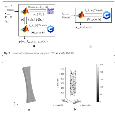
The integrated DVC code, Correli 3.0 [79], is a Matlab implementation that uses in a non-intrusive way a finite element code to compute the spatiotemporal sensitivity fields (Fig.2a) in addition to the current estimates of the displacement fields and reaction forces. The inputs to such simulations are the measured displacements of some boundaries of the ROI. In the present case, the commercial finite element package Abaqus/Standard is used with its built-in constitutive laws. C++ kernels compute all the other data needed to perform DVC analyses, namely, the DVC matrix [M], the instantaneous voxel residuals
ρ(x, t), and the instantaneous nodal residual vector{b(t)}. Binary MEX files are generated and called in the Matlab environment to compute the Hessians and residual vectors to be utilized in the Gauss–Newton schemes introduced above.
Fig. 2 Numerical implementation. Integrated DVC (a) and T4-DVC (b)
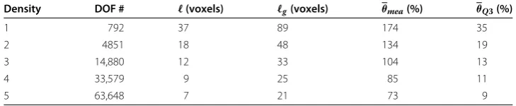
Fig. 3 Reconstructed volume in the reference configuration. 3D rendering of the thresholded volume (a) and gray level orthoslice (b) in which the ferritic-pearlitic matrix appears in light levels and the graphite nodules in dark
Results and discussion In situ mechanical test
Figure3shows the reconstructed volume in the reference configuration (i.e.,F=165 N). The coarse microstructure of cast iron can be observed in which the graphite nodules appear dark and the ferritic-pearlitic matrix in light gray levels. This is due to the fact that the X-ray absorption of iron is significantly higher than that of carbon. The mean volume fraction of nodules is equal to 15%.
Mesh of the ROI
Fig. 4 H8 and T4 meshes for a density of 1.aH8 mesh adapted to the actual sample geometry. bCorresponding T4 mesh with the same number of nodes
Table 1 Different meshes studied in this work and their corresponding quality with measured and linearly interpolated boundary conditions
Density DOF # (voxels) g(voxels) θmea(%) θQ3(%)
1 792 37 89 174 35
2 4851 18 48 134 19
3 14,880 12 33 104 13
4 33,579 9 25 85 11
5 63,648 7 21 73 9
Finer meshes will also be considered in integrated analyses (Table1). For each mesh, two different equivalent lengths are given. The first one corresponds to the cubic root of the mean volume of the T4 elements. This quantitywas introduced for the evaluation of the measurement uncertainty when each T4 element is considered independently. However, to define the spatial resolution associated with displacement measurements of global DVC a second length is also evaluated. It corresponds to the cubic root of the mean number of voxels considered for the nodal displacement measurement. This lengthgdefines the spatial resolution of the measurement technique. Table1shows thatgis less than three times the element size.
Measured displacement fields
The root mean square (RMS) residual is equal to 6.5 gray levels, which is an estimate of acquisition and reconstruction noise (i.e.,√2γI).
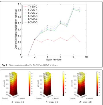
The T4-DVC code is then run incrementally to estimate the total displacements for the 9 analyzed steps. Figure5shows the change of the dimensionless RMS gray level residual
ρ2ROI/2γ2
I for all analyzed scans. These levels are virtually constant for the whole analysis except the first one where no motion has occurred between the two acquisitions. Furthermore the dimensionless residuals remain very close to 1 (i.e., an increase of 30% at most is obtained). This trend was also observed in C8-DVC and regularized C8-DVC (i.e., RC8-DVC) analyses [41].
Longitudinal displacement fields are reported in Fig.6for three different load levels. As the applied load level increases so do the displacement amplitudes. It is worth noting that even for the last load level no localization is observed. The material is presumably still in the hardening regime of plasticity.
Integrated DVC
In the sequel all reported results will consider displacement fields that are mechanically admissible in a finite element sense. Consequently, the first question to address is the
Fig. 5 Dimensionless residual for T4-DVC and I-DVC analyses
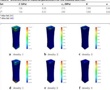
Table 2 Different sets of material parameters for the studied cast iron
Set E(GPa) ν σy(MPa) K n
1a 158 0.28 210 1300 0.44
2b 156 0.33 290 1260 0.62
aAfter Ref. [41] bAfter Ref. [40]
Fig. 7 Effect of mesh density and type of boundary conditions on local CRE errors. Local contributions to the error estimate for different mesh densities and for measured (top row) or linearly interpolated (bottom row) boundary conditions
quality of the finite element simulations. The next issues will be related to the analysis of the experiment per se. It is worth remembering that when finite element simulations are carried out, the material model and the parameters need to be known for cast iron. Two sets of parameters (see Table2) will be considered for Ludwik’s law (“Mesh of the ROI” section). The first one was obtainedviaweighted FEMU-UF [41] to analyze a cyclic tensile test on the same material at the macroscale. The second one was determined from the analysis of a standard monotonic tensile test [40].
Verification
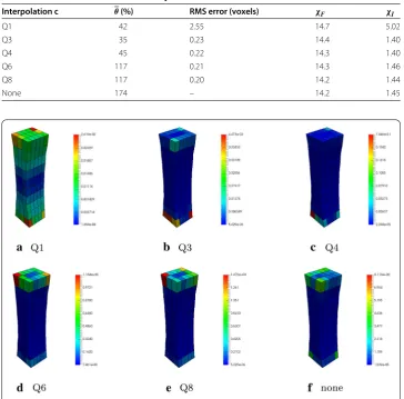
Table 3 Effect of the interpolation of boundary conditions on mesh quality and identification results for mesh density 1
Interpolation c θ(%) RMS error (voxels) χF χI
Q1 42 2.55 14.7 5.02
Q3 35 0.23 14.4 1.40
Q4 45 0.22 14.3 1.40
Q6 117 0.21 14.3 1.46
Q8 117 0.20 14.2 1.44
None 174 – 14.2 1.45
Fig. 8 Effect of boundary condition interpolations on local CRE errors. Local contributions to the error estimate for a given mesh (with density 1) but various interpolations of the boundary conditions
{1, x, y, xy, x2, y2, x2y, xy2}, wherexandydenote the two spatial coordinates over which the interpolation is performed. Therefore, Q1 corresponds to constant interpolation, Q3 to linear interpolation, and Q6 to quadratic interpolation. For a linear interpolation, there is a clear gain in terms of discretization errors when compared to the initial results (Fig.7). Table3shows that the RMS interpolation error between the measured displace-ments and their interpolations is very high for the uniform case (i.e., more than 36 times the standard displacement uncertainty). This is due to the fact that rigid body rotations are not accounted for. The interpolation errors for the other descriptions are close and significantly lower than in the previous case (i.e., of the order of 3 times the standard displacement uncertainty).
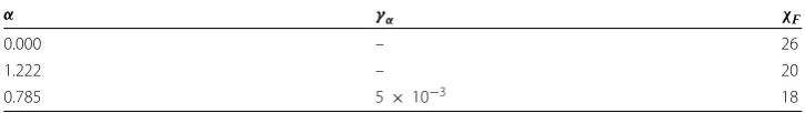
Table 4 Effect of displacement amplitudes on static residual for a mesh density of 1 and the first set of material parameters
α γα χF
0.000 – 26
1.222 – 20
0.785 5×10⁻³ 18
an eightfold gain is observed for mesh densities ranging from 3 to 5 (Table1). This result proves that most of the CRE errors are due to Dirichlet boundary conditions constructed with the measured displacement fields whose high frequency fluctuations are due to noise.
Boundary conditions
Since the reference scan was acquired for a load level equal to 165 N (Fig.1), the zero load configuration is not known. This lack of information is of no consequence when standard DVC analyses are run (i.e., C8-DVC and T4-DVC) or even regularized DVC. Conversely, when integrated approaches are performed in which the constitutive law is nonlinear, the zero load configuration has to be either known or estimated. In the present case, the second route has to be followed.
Since the measured displacement fieldsumeas(x, t−t0) have been evaluated with respect
to a nonzero load configuration (at timet0for which the load level is equal to 165 N), an
additional fieldu(x, t0) has to be added to get the experimental displacement from which
the Dirichlet boundary conditions are extracted to drive FE simulations
umeas(x, t)=umeas(x, t−t0)+u(x, t0) (45)
This additional field being unknown, it will be evaluated via FEMU-F. Since the first increment is elastic, it is assumed that
u(x, t0)=αumeas(x, t1−t0) (46)
wheret1corresponds to the 300-N load level, andαan unknown amplitude to be deter-mined.
For a mesh density of 1 and the first set of material parameters, Table4shows the effect of different values of the amplitudeαon the static residualχF. There is a clear influence of
αonχF, and more importantly, the standard uncertaintyγαis very low in comparison with the reported level ofα. The fact thatχFis significantly larger than unity is an indication of model errors. This first analysis allows the load residuals to be decreased from 26 (when
α = 0) to 18 whenα is optimized via the load residuals, which corresponds to a 30% decrease.
The next question to address is whether a more complex correction can be proposed. Instead of having the same amplitude on the longitudinal and transverse components, it is proposed to look for three different amplitudes αx,αy andαz for each direction. Before performing the identification, a sensitivity analysis is carried out [81]. It consists in computing the dimensionless static Hessian for a given variation of the sought parameters (here chosen equal to 10%)
[HF]= 1
ntnFγF2
[δF]†[δF] (47)
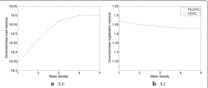
Fig. 9 Effect of mesh density on I-DVC results. Load (a) and registration (b) residuals as functions of mesh density for the first set of material parameters
equal to 1 will more sensitive than the noise level. The load cell of the testing machine used herein has a standard uncertainty equal to 3.5 N. In the present case, the dimensionless static Hessian reads
[HF]=
⎡ ⎢ ⎢ ⎣
4×10⁻³ −2×10⁻³ −34×10−3
−2×10⁻³ 3×10⁻³ 76×10−3
−34×10−3 76×10−3 2.247
⎤ ⎥ ⎥
⎦ (48)
and has only one eigen value greater than 1. The corresponding eigen vector is essentially aligned with the third parameter direction (i.e.,αz). The other two eigen values are at least three orders of magnitude lower. The new parameterization is therefore not sensitive enough with the data at hand. Similarly, when αx andαy are assumed to be identical, the largest eigen value is greater than 1 and its eigen direction is again aligned with the direction of αz. The second eigen value is three orders of magnitude lower. This last parameterization is not compatible with the available information. Consequently only the first one is considered hereafter.
Effect of mesh density
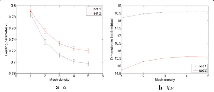
Fig. 10 Values ofαandχFfor two different sets of material parameters and five mesh densities. Theerror barsindicate the standard deviationγαfor each identified value
history of instantaneous dimensionless registration residuals is again analyzed (Fig. 5). Contrary to T4-DVC it is observed that the registration quality degrades as the scan number increases, i.e., more yielding has occurred. The fact that this trend is identical for all five mesh densities is an indication of a material model error and not a discretization error. To obtain the results discussed in this section the computation time ranges from a few minutes for mesh density 1 to two hours for the finest mesh on a workstation (with 2.6-GHz Intel Xeon E5-2650 processor). Let us emphasize that this computation time remains small as compared to the duration of the experiment, and even smaller if preparation time is considered.
Comparison of two sets of material parameters
Having based 4D registrations on a single set of material parameters, the next question to address is their influence on the results. A second set of parameters (see Table 2) is used in the same analysis as in the previous sections. Figure10shows the values of the unknown loading parameter α as functions of the mesh densities for the two sets of material parameters when using FEMU-F. This convergence analysis shows that for the two sets of material parameters, the mesh densities 4 and 5 lead to approximately the same value ofα andχF. There is a small influence (i.e., less than 3%) of the set of material parameters on the value for the finest meshes. This is to be expected since the first load level is assumed to be elastic and the corresponding Young’s moduli are very close. Further, the standard uncertaintyγαdecreases by about 15% from density 1 to 5.
Table5shows the load and registration residuals for the two sets of material parameters. For the load residual, the second set of material parameters is better than the first one. There is a clear sensitivity ofχFto the two sets. It is worth noting that the finer the meshes the sightly higher the load residuals in both cases. For the registration residuals, the first set of material parameters is better than the second one. This is also true for the global residualχ. These results indicate that even though the number of scans is very small (i.e., less than ten), the two residuals are sensitive to the material parameters.
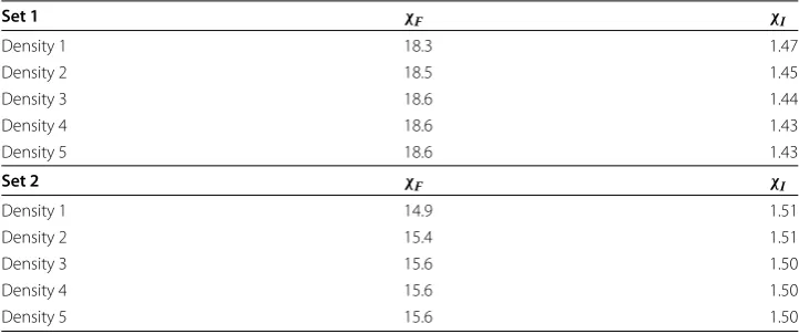
Table 5 Static and registration residuals for the two sets of material parameters and different mesh densities
Set 1 χF χI
Density 1 18.3 1.47
Density 2 18.5 1.45
Density 3 18.6 1.44
Density 4 18.6 1.43
Density 5 18.6 1.43
Set 2 χF χI
Density 1 14.9 1.51
Density 2 15.4 1.51
Density 3 15.6 1.50
Density 4 15.6 1.50
Density 5 15.6 1.50
Table 6 Material parameters determined via FEMU-F. Static, registration and global residuals for different mesh densities
Density σy(MPa) K(MPa) n χF χI
1 250±6 1300±109 0.55±0.03 14.17 1.49
2 258±7 1300±160 0.57±0.05 14.20 1.48
3 257±2 1300±40 0.57±0.01 14.27 1.46
4 256±5 1300±83 0.57±0.03 14.30 1.46
5 256±7 1300±140 0.57±0.04 14.31 1.45
Identification of material parameters
In the following, only the plastic parameters (i.e.,σy,Kandn) are identified. By performing the same sensitivity analysis as in “Boundary conditions” section, it is concluded that two eigen values of [HF] are greater than 1 for a parameter variation of 10%. Instead of setting the least sensitive parameter to its initial guess, a Tikhonov-type of regularization [82] is preferred. It consists in adding a penalization term from the initial guess{p0}of the sought parameters, say in the FEMU-F procedure,
[HF]+λF[I]{δp} =
t
[SF(t)]†{Fmeas(t)−FEF(t,{p})} +λF({p0} − {p}) (49) whereλF is set in such a way that at the end of the relaxation procedure is has the same order of magnitude as the second eigen value of [HF]. The relaxation procedure [59] consists in iterating the present scheme by starting with λF equal to one thousandth of the maximum eigen value of [HF]. Once convergence is reached (i.e., each relative parameter variation is less than 10−5), the regularization lengthλFis divided by ten and the procedure is repeated untilλF has the same order of magnitude as the second eigen value.
Fig. 11 Identification results for five mesh densities. Values ofχI(a) andχF(b) at convergence of the FEMU-F procedure
Fig. 12 Effect of the interpolation of the Dirichlet boundary conditions on the identified material parameters (mesh density: 1). The reference set of parameters is that when no interpolation is applied to the measured boundary conditions
acquisition noise. However, it is lower than what was observed for the two sets of material parameters (Table5).
Figure11shows an opposite dependence of the two identification residuals with the mesh density. However, the relative variations ofχF are smaller than those observed for the two sets of parameters (Table5). Conversely,χIis slightly more sensitive to the mesh density.
Fig. 13 Identification results via 4D registration.aFinest mesh used in the present study (density: 5). bOrthoslice of the gray level residuals of scan #9.cComparison of measured and predicted load levels
the same density. The material parameters are not significantly altered in comparison to the identified values reported in Table6.
Sensitivity to boundary conditions
In the following, only the linear interpolation is studied for the different mesh densi-ties. When the load and registration residuals are computed for all these cases with the same material parameters (identified when the measured boundary conditions are con-sidered), the registration residuals are identical and the load residuals slightly increase with the mesh density as already observed (see Fig.11). These results indicate that the identification procedure does not need such fine meshes. One of the reasons of this result is likely to be related to the fact that the load residuals are still very high (i.e., there is a significant model error). Figure13summarizes the identification results for the finest mesh (i.e., leading to the smallest CRE error). The gray level residuals are very low in com-parison with the reference microstructure (see Fig.3b). This is an additional proof that the registration is successful not only globally but also locally. When the measured load history is compared to the corresponding predictions, higher differences are observed. This result is to be expected from the global residuals, which are significantly higher than the measurement uncertainties.
Conclusions
It has been shown herein that full integration of sensor and measurement data can be achieved in numerical procedures via so-called 4D mechanical correlation. In the present case, load measurements are combined with reconstructed volumes thanks to computed tomography. Local and global residuals have been constructed in which each measured or predicted result is compared to the corresponding noise level. In 4D registrations, the mechanical finite element code was utilized in a non-intrusive way to generate elastoplas-tic fields. This type of approach is very generic and can be deployed under very different conditions.
Within the proposed framework, uncertainty quantifications have been carried out for the measured kinematic degrees of freedom and the sought parameters. For incremental correlation procedures, it is shown that the finer the mesh, the more uncertain the mea-sured quantities. This trend is opposite to that of verification procedures where refined meshes better capture mechanical fields. This limitation can be overcome by considering kinematic fields that are mechanically admissible, i.e., to integrated DVC (i.e., 4D mechan-ical correlation). Consequently, convergence studies can be conducted when dealing with experimental data.
Alternative 4D routes may be considered as well. For instance, by resorting to projection-based registration procedures [48], it is possible to reduce the number of projections needed to evaluate 3D kinematic fields. When extended to (many) more time steps, it would allow the experimentalist not to interrupt the test and acquire the radiographs on the fly. A truly 4D formulation would be required in which reconstruction and registration procedures would be coupled with mechanically admissible fields.
Another direction of progress can be envisioned thanks to the scale at which microto-mography is performed, namely, the study of the mechanical behavior at the microscale. For the studied material, this would allow the behavior of the ferrite/pearlite matrix to be analyzed in conjunction with the debonding of the interface between the brittle nod-ules and their surrounding matrix. The same framework as that introduced herein can be used. However, the meshes will needed to be significantly finer and adapted to the microstructure [58].
Authors’ contributions
AB and ZT carried out the in-situ test. FP and LC performed the verification analyses. The computational framework (Correli 3.0) was implemented by HL, FM and JN. FH wrote all the I-DVC routines within the Correli 3.0 framework. SR and FH introduced the theoretical background and performed the uncertainty quantifications. All authors read and approved the final manuscript.
Author details
1LMT, ENS Cachan/CNRS/Université Paris-Saclay, 61 Avenue du Président Wilson, Cachan, France ,2Department of
Engineering Mechanics, Faculty of Mechanical Engineering and Naval Architecture, University of Zagreb, Luˇci´ca 5, Zagreb, Croatia,3Laboratoire Modélisation et Simulation Multi Echelle MSME UMR 8208 CNRS, Université Paris-Est,
5 Boulevard Descartes, Marne-la-Vallée, France.
Acknowledgements
This work was supported by BPI France (DICCIT project) and by the French “Agence Nationale de la Recherche” through the “Investissements d’avenir” program (ANR-10-EQPX-37 MATMECA grant). ZT thanks Campus France for supporting his stay at LMT through an Eiffel scholarship.
Competing interests
The authors declare that they have no competing interests.
Received: 23 February 2016 Accepted: 27 April 2016
References
1. Oden JT, Belytschko T, Fish J, Hughes TJR, Johnson C, Keyes D, Laub A, Petzold L, Srolovitz D, Yip S. Simulation-based engineering sciences. Final report, NFS. 2006.http://www.nsf.gov/pubs/reports/sbes_final_report
2. Avril S, Bonnet M, Bretelle AS, Grédiac M, Hild F, Ienny P, Latourte F, Lemosse D, Pagano S, Pagnacco E, Pierron F. Overview of identification methods of mechanical parameters based on full-field measurements. Exp Mech. 2008;48(4):381–402.
3. Rannou J, Limodin N, Réthoré J, Gravouil A, Ludwig W, Baïetto MC, Buffière JY, Combescure A, Hild F, Roux S. Three dimensional experimental and numerical multiscale analysis of a fatigue crack. Comp Meth Appl Mech Eng. 2010;199:1307–25.
4. Baruchel J, Buffière JY, Maire E, Merle P, Peix G, editors. X-ray tomography in material sciences. Paris: Hermès Science; 2000.
5. Salvo L, Cloetens P, Maire E, Zabler S, Blandin JJ, Buffiere JY, Ludwig W, Boller E, Bellet D, Josserond C. X-ray micro-tomography an attractive characterisation technique in materials science. Nucl Instr Meth Phys Res B. 2003;200:273– 86.
6. Desrues J, Viggiani G, Bésuelle P, editors. Advances in X-ray tomography for geomaterials. London: Wiley / ISTE; 2006. 7. Stock SR. Recent advances in X-Ray microtomography applied to materials. Int Mat Rev. 2008;53(3):129–81. 8. Maire E, Withers PJ. Quantitative X-ray tomography. Int Mat Rev. 2014;59(1):1–43.
9. Desrues J, Chambon R, Mokni M, Mazerolle MF. Void ratio evolution inside shear bands in triaxial sand specimens studied by computed tomography. Géotechnique. 1996;46(3):529–46.
10. Guvenilir A, Breunig TM, Kinney JH, Stock SR. Direct observation of crack opening as a function of applied load in the interior of a notched tensile sample of Al-Li 2090. Acta Mater. 1997;45(5):1977–87.
11. Buffière JY, Maire E, Cloetens P, Lormand G, Fougères R. Characterisation of internal damage in a MMCp using X-ray synchrotron phase contrast microtomography. Acta Mater. 1999;47(5):1613–25.
12. Buffière JY, Maire E, Adrien J, Masse JP, Boller E. In situ experiments with X ray tomography: an attractive tool for experimental mechanics. Exp Mech. 2010;50(3):289–305.
14. Babout L, Maire E, Fougères R. Damage initiation in model metallic materials: X-ray tomography and modelling. Acta Mater. 2004;52:2475–87.
15. Pyzalla A, Camin B, Buslaps T, Di Michiel M, Kaminski H, Kottar A, Pernack A, Reimers W. Simultaneous tomography and diffraction analysis of creep damage. Science. 2005;308(5718):92–5.
16. Isaac A, Sket F, Reimers W, Camin B, Sauthoff G, Pyzalla AR. In situ 3D quantification of the evolution of creep cavity size, shape, and spatial orientation using synchrotron X-ray tomography. Mat Sci Eng A. 2008;478(1–2):108–18. 17. Huppmann M, Camin B, Pyzalla AR, Reimers W. In-situ observation of creep damage evolution in Al-Al2O3MMCs by
synchrotron X-ray microtomography. Int J Mat Res. 2010;101:372–9.
18. Borbély A, Dzieciol K, Sket F, Isaac A, di Michiel M, Buslaps T, Kaysser-Pyzalla AR. Characterization of creep and creep damage by in-situ microtomography. JOM. 2011;63(7):78–84.
19. Bay BK, Smith TS, Fyhrie DP, Saad M. Digital volume correlation: three-dimensional strain mapping using X-ray tomography. Exp Mech. 1999;39:217–26.
20. Smith TS, Bay BK, Rashid MM. Digital volume correlation including rotational degrees of freedom during minimization. Exp Mech. 2002;42(3):272–8.
21. Limodin N, Réthoré J, Buffière JY, Gravouil A, Hild F, Roux S. Crack closure and stress intensity factor measure-ments in nodular graphite cast iron using 3D correlation of laboratory X ray microtomography images. Acta Mat. 2009;57(14):4090–101.
22. Limodin N, Réthoré J, Buffière JY, Hild F, Roux S, Ludwig W, Rannou J, Gravouil A. Influence of closure on the 3D propagation of fatigue cracks in a nodular cast iron investigated by X-ray tomography and 3D volume correlation. Acta Mat. 2010;58(8):2957–67.
23. Limodin N, Réthoré J, Adrien J, Buffière JY, Hild F, Roux S. Analysis and artifact correction for volume correlation measurements using tomographic images from a laboratory X-ray source. Exp Mech. 2011;51(6):959–70.
24. Morgeneyer TF, Helfen L, Mubarak H, Hild F. 3D digital volume correlation of synchrotron radiation laminography images of ductile crack initiation: an initial feasibility study. Exp Mech. 2013;53(4):543–56.
25. Allix O, Feissel P, Nguyen HM. Identification strategy in the presence of corrupted measurements. Eng Comput. 2005;22(5–6):487–504.
26. Feissel P, Allix O. Modified constitutive relation error identification strategy for transient dynamics with corrupted data: the elastic case. Comput Meth Appl Mech Eng. 2007;196(13/16):1968–83.
27. Latourte F, Chrysochoos A, Pagano S, Wattrisse B. Elastoplastic behavior identification for heterogeneous loadings and materials. Exp Mech. 2008;48(4):435–49.
28. Pierron F, Grédiac M. The virtual fields method. New York: Springer; 2012.
29. Claire D, Hild F, Roux S. A finite element formulation to identify damage fields: the equilibrium gap method. Int J Num Meth Eng. 2004;61(2):189–208.
30. Hild F, Roux S. Digital image correlation: from measurement to identification of elastic properties-a review. Strain. 2006;42:69–80.
31. Roux S, Hild F. Stress intensity factor measurements from digital image correlation: post-processing and integrated approaches. Int J Fract. 2006;140(1–4):141–57.
32. Leclerc H, Périé JN, Roux S, Hild F. In: Gagalowicz A, Philips W, editors. Integrated digital image correlation for the identification of mechanical properties, vol. LNCS 5496. Berlin: Springer; 2009. p. 161–71.
33. Réthoré J. A fully integrated noise robust strategy for the identification of constitutive laws from digital images. Int J Num Meth Eng. 2010;84(6):631–60.
34. Réthoré J. Muhibullah, Elguedj T, Coret M, Chaudet P, Combescure A. Robust identification of elasto-plastic constitutive law parameters from digital images using 3D kinematics. Int J Solids Struct. 2013;50(1):73–85.
35. Dufour J-E, Hild F, Roux S. Shape, displacement and mechanical properties from isogeometric multiview stereocorre-lation. J Strain Anal. 2015;50(7):470–87.
36. Neggers J, Hoefnagels JPM, Geers MGD, Hild F, Roux S. Time-resolved integrated digital image correlation. Int J Num Meth Eng. 2015;203(3):157–82.
37. Bouterf A, Roux S, Hild F, Adrien J, Maire E. Digital volume correlation applied to X-ray tomography images from spherical indentation tests on lightweight gypsum. Strain. 2014;50(5):444–53.
38. Tarantola A. Inverse problems theory. Methods for data fitting and model parameter estimation. Southampton: Elsevier Applied Science; 1987.
39. Mathieu F, Leclerc H, Hild F, Roux S. Estimation of elastoplastic parameters via weighted FEMU and integrated-DIC. Exp Mech. 2015;55(1):105–19.
40. Tomiˇcevi´c Z. Identification of the mechanical properties of nodular graphite cast iron via multiaxial tests. PhD thesis. 2015.
41. Tomiˇcevi´c Z, Kodvanj J, Hild F. Characterization of the nonlinear behavior of nodular graphite cast iron via inverse identification. Analysis of uniaxial tests. Europ J Mech A/Solids. 2016;59:140–54.
42. Sutton MA. Computer vision-based, noncontacting deformation measurements in mechanics: a generational trans-formation. Appl Mech Rev. 2013;65(AMR–13–1009):050802.
43. Sutton MA, Hild F. Recent advances and perspectives in digital image correlation. Exp Mech. 2015;55(1):1–8. 44. Bornert M, Chaix JM, Doumalin P, Dupré JC, Fournel T, Jeulin D, Maire E, Moreaud M, Moulinec H. Mesure
tridimen-sionnelle de champs cinématiques par imagerie volumique pour l’analyse des matériaux et des structures. Inst Mes Métrol. 2004;4:43–88.
45. Verhulp E, van Rietbergen B, Huiskes R. A three-dimensional digital image correlation technique for strain measure-ments in microstructures. J Biomech. 2004;37(9):1313–20.
46. Roux S, Hild F, Viot P, Bernard D. Three dimensional image correlation from X-Ray computed tomography of solid foam. Comp Part A. 2008;39(8):1253–65.
47. Leclerc H, Périé JN, Hild F, Roux S. Digital volume correlation: What are the limits to the spatial resolution? Mech Indust. 2012;13:361–71.
49. Kak AC, Slaney M. Principles of computerized tomographic imaging, Society of Industrial and Applied Mathematics. 2001.
50. Hild F, Fanget A, Adrien J, Maire E, Roux S. Three dimensional analysis of a tensile test on a propellant with digital volume correlation. Arch Mech. 2011;63(5–6):1–20.
51. Lucas BD, Kanade T. An iterative image registration technique with an application to stereo vision. In: 7th international joint conference on artificial intelligence. 1981. p. 674–79.
52. Fedele R, Galantucci L, Ciani A. Global 2D digital image correlation for motion estimation in a finite element framework: a variational formulation and a regularized, pyramidal, multi-grid implementation. Int J Num Meth Eng. 2013;96(12):739–62.
53. Hild F, Roux S. In: Rastogi P, Hack E, editors. Digital image correlation. Weinheim: Wiley-VCH; 2012. p. 183–228. 54. Hild F, Roux S. Comparison of local and global approaches to digital image correlation. Exp Mech. 2012;52(9):1503–19. 55. Maire E, Fazekas A, Salvo L, Dendievel R, Youssef S, Cloetens P, Letang JM. X-ray tomography applied to the
charac-terization of cellular materials related finite element modeling problems. Compos Sci Tech. 2003;63(16):2431–43. 56. Youssef S, Maire E, Gaertner R. Finite element modelling of the actual structure of cellular materials determined by
x-ray tomography. Acta Mater. 2005;53(3):719–30.
57. Zhang Y, Bajaj C, Sohn BS. 3D finite element meshing from imaging data. Comput Meth Appl Mech Eng. 2005;194(48– 49):5083–106.
58. Shakoor M, Bouchard PO, Bernacki M. An adaptive level-set method with enhanced volume conservation for simula-tions in multiphase domains. Int J Num Meth Eng. 2016.(accepted for publication).
59. Gras R, Leclerc H, Hild F, Roux S, Schneider J. Identification of a set of macroscopic elastic parameters in a 3d woven composite: uncertainty analysis and regularization. Int J Solids Struct. 2015;55:2–16.
60. Babu˘ska I, Rheinboldt WC. Error estimates for adaptive finite element computation. SIAM J Num Anal. 1978;15(4):736– 54.
61. Ladevèze P, Leguillon D. Error estimate procedure in the finite element method and applications. SIAM J Num Anal. 1983;20(3):485–509.
62. Zienkiewicz OC, Zhu JZ. A simple error estimator and adaptive procedure for practical engineerng analysis. Int J Num Meth Eng. 1987;24(2):337–57.
63. Ladevèze P, Moës N. A new a posteriori error estimation for nonlinear time-dependent finite element analysis. Comp Meth Appl Mech Eng. 1998;157:45–68.
64. Destuynder P, Métivet B. Explicit error bounds in a conforming finite element method. Math Comput. 1999;68(288):1379–96.
65. Ladevèze P, Pelle J. Mastering calculations in linear and nonlinear mechanics. New York: Springer; 2004.
66. Chamoin L, Diez P. Verifying calculations, forty years on: an overview of classical verification techniques for FEM simulations. Switzerland: Springer; 2015.
67. Ludwik P. Elemente der Technologischen Mechanik. Leipzig: Verlag Von Julius Springer; 1909. 68. Germain P, Nguyen QS, Suquet P. Continuum thermodynamics. ASME J Appl Mech. 1983;50:1010–20. 69. Lemaitre J, Chaboche JL. Mechanics of solid materials. Cambridge: Cambridge University Press; 1990.
70. Prager W, Synge JL. Approximation in elasticity based on the concept of functions spaces. Q Appl Math. 1947;5:261–9. 71. Pled F, Chamoin L, Ladevèze P. On the techniques for constructing admissible stress fields in model verification:
performances on engineering examples. Int J Num Meth Eng. 2011;88(5):409–41.
72. Taillandier-Thomas T, Roux S, Morgeneyer TF, Hild F. Localized strain field measurement on laminography data with mechanical regularization. Nucl Inst Meth Phys Res B. 2014;324:70–9.
73. Leclerc H, Périé JN, Roux S, Hild F. Voxel-scale digital volume correlation. Exp Mech. 2011;51(4):479–90.
74. Perini LAG, Passieux J-C, Périé J-N. A multigrid PGD-based algorithm for volumetric displacement fields measurements. Strain. 2014;50(4):355–67.
75. Besnard G, Guérard S, Roux S, Hild F. A space-time approach in digital image correlation: movie-DIC. Optics Lasers Eng. 2011;49:71–81.
76. Besnard G, Leclerc H, Roux S, Hild F. Analysis of image series through digital image correlation. J Strain Anal. 2012;47(4):214–28.
77. Collins JD, Hart GC, Hasselman TK, Kennedy B. Statistical identification of structures. AIAA J. 1974;12(2):185–90. 78. Pagnacco E, Caro-Bretelle AS, Ienny P. In: Grédiac M, Hild F, editors. Parameter identification from mechanical field
measurements using finite element model updating strategies. London: ISTE / Wiley; 2012. p. 247–74.
79. Leclerc H, Neggers J, Mathieu F, Hild F, Roux S. Correli 3.0. IDDN.FR.001.520008.000.S.P.2015.000.31500, Agence pour la Protection des Programmes, Paris; 2015.
80. Babu˘ska I, Strouboulis T. The finite element method and its reliability. Oxford: Oxford University Press; 2001. 81. Bertin M, Hild F, Roux S, Mathieu F, Leclerc H, Aimedieu P. Integrated digital image correlation applied to elasto-plastic
identification in a biaxial experiment. J Strain Anal. 2016;51(2):118–31.