04 August 2020
Integration of Active Systems for a Global Chassis Control Design / Tota, Antonio. - (2017). Original
Integration of Active Systems for a Global Chassis Control Design
Publisher:
Published
DOI:10.6092/polito/porto/2675382 Terms of use:
Altro tipo di accesso
Publisher copyright
(Article begins on next page)
This article is made available under terms and conditions as specified in the corresponding bibliographic description in the repository
Availability:
This version is available at: 11583/2675382 since: 2017-06-30T10:47:37Z Politecnico di Torino
Integration of Active Systems for a
Global Chassis Control Design
By
Antonio Tota
****** Supervisor(s):
Prof. Mauro Velardocchia, Supervisor
Doctoral Examination Committee:
Prof. Giuseppe Carbone, Referee, Università degli Studi di Cassino Prof. Alessandro Gasparetto, Referee, Università degli Studi di Udine Prof. Enrico Ravina, Università degli Studi di Genova
Prof. Giuseppe Quaglia, Politecnico di Torino Prof. Vladimir Viktorov, Politecnico di Torino
Politecnico di Torino 2017
I hereby declare that, the contents and organization of this dissertation constitute my own original work and does not compromise in any way the rights of third parties, including those relating to the security of personal data.
Antonio Tota 2017
* This dissertation is presented in partial fulfillment of the requirements forPh.D. degree in the Graduate School of Politecnico di Torino (ScuDo).
e alle mie nonne, Ida e Rosa
La presente tesi di dottorato rappresenta il risultato finale di un lungo ed impegnativo percorso di ricerca durato tre anni, che non sarebbe stato tale senza il supporto, la collaborazione e l’aiuto di molte persone alle quali vorrei rivolgere i miei più sinceri ringraziamenti.
Il percorso universitario rappresenta per tutti una prova impegnativa e piena di osta-coli durante la quale bisogna imparare a conoscere se stessi ed il mondo che ci circonda, ma le oltre 200 pagine raccolte in questa tesi non basterebbero da sole a descrivere a pieno il sostegno e l’aiuto che ogni figlio/fratello vorrebbe ricevere dalla propria famiglia per il raggiungimento di obbiettivi personali e traguardi fondamentali per la propria vita. Io sono riuscito ad affrontarlo grazie alla presenza delle tre persone più importanti della mia vita: Benedetto, Loredana e Giuseppe Luca. Loro, che mi sono stati vicini anche quando ero lontano migliaia di chilometri dalla nostra amata/odiata Taranto, mi hanno trasmesso la forza per crederci sempre e la volontà di andare avanti senza mai guardare indietro. Mio padre Benedetto mi ha insegnato il rispetto per se stessi e per gli altri aiutandomi nelle scelte più difficili: sono estremamente fortunato di ricevere i suoi consigli. Mia madre Loredana è riuscita a rassicurarmi e a rasserenarmi durante i momenti più tristi e difficili, senza mai stancarsi di ripetere quanto fosse importante non sottovalutare i traguardi già raggiunti e cercando di spronarmi per raggiungerne degli altri. Giuseppe Luca, invece, non è più il fratellino minore da proteggere, ma una persona responsabile ed autonoma capace di gestirsi la vita ed in grado di trasmettere la sua sicurezza anche ad un fratello sbadato e disorganizzato come me, concedendomi talvolta anche le sue note doti culinarie. Spero che i sacrifici fatti e gli obbiettivi raggiunti durante questi anni vi renderanno orgogliosi e fieri di me.
Il lavoro di ricerca non sarebbe stato possibile e realizzabile senza la guida e la supervisione del Prof. Velardocchia che, con grande passione e fiduciosa aspettativa, insieme al Prof. Vigliani e all’Ing. Galvagno, conduce interessanti progetti di ricerca all’avanguardia nell’innovazione scientifica ed in collaborazione con importanti aziende legate al mondo automotive, per rimanere sempre al passo con le realtà industriali.
Un immenso ed impagabile ringraziamento è riservato per la mia amata Agathe che, oltre ad aver sopportato le numerose lamentele durante questi 3 anni di dottorato, ha sempre creduto nelle mie capacità incoraggiando i miei sforzi sia nei momenti di difficoltà che in quelli di felicità e spensieratezza. Neanche un oceano intero è riuscito a tenerti lontana da me: mi hai raggiunto in ogni posto sperduto del mondo in cui andavo a finire, trasformando la distanza in momenti straordinari ed indimenticabili. Merci beaucoup, ma belle!
Inoltre vorrei ringraziare il Prof. Aldo Sorniotti per avermi ospitato all’interno del suo team presso l’University of Surrey (Guildford, UK), e per avermi inserito all’interno di un progetto di ricerca che per me è stato un momento di vero apprendimento nel verificare concetti teorici attraverso prove sperimentali su pista davvero stimolanti oltre che divertenti. Un grazie speciale va anche a tutti gli amici del SAVAG ed i frequentatori di Stoke House che hanno saputo rendere indimenticabile il mio periodo trascorso a Guildford; un particolare grazie a Fabio, Daniele, Basilio, Stefano, Tommaso, Michele, Ilhan, Ventura per le serate trascorse insieme al Wetherspoons.
Sentiti e sinceri ringraziamenti sono dovuti anche agli attuali e vecchi membri del team di meccanica del veicolo (Guido, Pablo, Alberto, Mariangela, Hamid, Sara ed An-drea), con cui ho condiviso momenti di quotidianità al Politecnico di Torino e divertenti cene/pranzi/panzerottate in giro per Torino.
Uno speciale ringraziamento è rivolto anche al Prof. Rizzoni e al Prof. Guvenc per avermi invitato presso il Center for Automotive Research (CAR) dell’Ohio State Univer-sity (Columbus, OH), concedendomi l’opportunità di passare un’ulteriore esperienza internazionale ed interculturale che mi ha aiutato molto a perfezionare le mie abilità di lavoro di squadra grazie alla collaborazione con i componenti del Automated Driving Lab (ADL) Prof. Bilin Aksun-Guvenc, Santhosh, Nitish, Hongliang e Haoan. Vorrei anche inviare un saluto ed un ringraziamento a Matilde ed a Martin per tutti i momenti di divertimento e svago trascorsi insieme per le vie di Columbus.
Infine, last but not least, vorrei ricordare con un saluto tutti gli amici di Taranto e Torino che mi hanno sempre accompagnato durante i momenti di svago e di totale felicità, rappresentando sempre un punto di riferimento da cui trarre forza e sostegno per superare gli ostacoli della vita.
Grazie!
Vehicle chassis control active systems (braking, suspension, steering and driveline), from the first ABS/ESC control unit to the current advanced driver assistance systems (ADAS), are progressively revolutionizing the way of thinking and designing the vehicle, improving its interaction with the surrounding world (V2V and V2X) and have led to excellent results in terms of safety and performances (dynamic behavior and drivability). They are usually referred asintelligent vehiclesdue to a software/hardware architecture able to assist the driver for achieving specific safety margin and/or optimal vehicle dynamic behavior. Moreover, industrial and academic communities agree that these technologies will progress till the diffusion of the so called autonomous cars which are able to drive robustly in a wide range of traffic scenarios. Different autonomous vehicles are already available in Europe, Japan and United States and several solutions have been proposed for smart cities and/or small public area like university campus.
In this context, the present research activity aims at improving safety, comfort and performances through the integration of global active chassis control: the purposes are to study, design and implement control strategies to support the driver for achieving one or more final target among safety, comfort and performance. Specifically, the vehicle subsystems that are involved in the present research for active systems development are the steering system, the propulsion system, the transmission and the braking system. The thesis is divided into three sections related to different applications of active systems that, starting from a robust theoretical design procedure, are strongly supported by objective experimental results obtained from Hardware In the Loop (HIL) test rigs and/or proving ground testing sessions.
The first chapter is dedicated to one of the most discussed topic about autonomous driving due to its impact from the social point of view and in terms of human error mitigation when the driver is not prompt enough. In particular, it is here analyzed the automated steering control which is already implemented for automatic parking and that could represent also a key element for conventional passenger car in emergency situation where a braking intervention is not enough for avoiding an imminent collision. The activity is focused on different steering controllers design and their implementation
for an autonomous vehicle; an obstacle collision avoidance adaptation is introduced for future implementations. Three different controllers, Proportional Derivative (PD), PD+Feedforward (FF) e PD+Integral Sliding Mode (ISM), are designed for tracking a reference trajectory that can be modified in real-time for obstacle avoidance purposes. Furthermore, PD+FF and PD+ISM logic are able to improve the tracking performances of automated steering during cornering maneuvers, relevant from the collision avoidance point of view. Path tracking control and its obstacle avoidance enhancement is also shown during experimental tests executed in a proving ground through its implemen-tation for an autonomous vehicle demonstrator. Even if the activity is presented for an autonomous vehicle, the active control can be developed also for a conventional vehicle equipped with an Electronic Power Steering (EPS) or Steer-by-wire architectures.
The second chapter describes a Torque Vectoring (TV) control strategy, applied to a Fully Electric Vehicle (FEV) with four independent electric motor (one for each wheel), that aims to optimize the lateral vehicle behavior by a proper electric motor torque regulation. A yaw rate controller is presented and designed in order to achieve a desired steady-state lateral behaviour of the car (handling task). Furthermore, a sideslip angle controller is also integrated to preserve vehicle stability during emergency situations (safety task). LQR, LQR+FF and ISM strategies are formulated and explained for yaw rate and concurrent yaw rate/sideslip angle control techniques also comparing their advantages and weakness points. The TV strategy is implemented and calibrated on a FEV demonstrator by executing experimental maneuvers (step steer, skid pad, lane change and sequence of step steers) thus proving the efficacy of the proposed controller and the safety contribution guaranteed by the sideslip control. The TV could be also applied for internal combustion engine driven vehicles by installing specific torque vectoring differentials, able to distribute the torque generated by the engine to each wheel independently.
The TV strategy evaluated in the second chapter can be influenced by the presence of a transmission between the motor (or the engine) and wheels (where the torque control is supposed to be designed): in addition to the mechanical delay introduced by transmis-sion components, the presence of gears backlashes can provoke undesired noises and vibrations in presence of torque sign inversion. The last chapter is thus related to a new method for noises and vibration attenuation for a Dual Clutch Transmission (DCT). This is achieved in a new way by integrating the powertrain control with the braking system control, which are historically and conventionally analyzed and designed separately. It is showed that a torsional preload effect can be obtained on transmission components by increasing the wheel torque and concurrently applying a braking wheel torque. For this reason, a pressure following controller is presented and validated through a Hardware In
the Loop (HIL) test rig in order to track a reference value of braking torque thus ensuring the desired preload effect and noises reduction. Experimental results demonstrates the efficacy of the controller, also opening new scenario for global chassis control design.
Finally, some general conclusions are drawn and possible future activities and rec-ommendations are proposed for further investigations or improvements with respect to the results shown in the present work.
Abstract vi
List of Figures xii
List of Tables xx
1 Autonomous Steering Control 1
1.1 Introduction on Autonomous Steering Driving . . . 1
1.2 Experimental Setup of the Autonomous Vehicle . . . 5
1.3 Single-Track Model . . . 7
1.3.1 Dynamics equations . . . 8
1.3.2 Steady-State behavior . . . 11
1.3.3 Experimental Validation . . . 13
1.3.4 Steering Dynamics Model . . . 21
1.3.5 Lateral Deviation Equations . . . 24
1.4 Path Tracking Control . . . 26
1.4.1 Reference Path Generation . . . 26
1.4.2 Parameter Space Approach: Theory and Application . . . 32
1.4.3 Static Linear Feedforward . . . 51
1.4.4 Integral Sliding Mode: Theory and Application . . . 52
1.4.5 Obstacle Collision Avoidance Path Modification . . . 63
1.5 Experimental Results . . . 66
1.5.2 Close-Loop Path for Obstacle Avoidance . . . 72
1.6 Conclusions . . . 74
2 Torque Vectoring Control for Fully-Electric Vehicles 76 2.1 Introduction on Torque Vectoring Theory . . . 76
2.2 Experimental Setup of the FEV demonstrator . . . 81
2.3 Control System Design . . . 83
2.3.1 Control structure . . . 84
2.3.2 Yaw rate and Sideslip references . . . 86
2.3.3 Yaw Moment Controller: Linear Quadratic Regulator Design . . . . 93
2.3.4 Yaw Moment Controller: Integral Sliding Mode Design . . . 97
2.4 Simulation Results . . . 103
2.4.1 High friction coefficient step steer . . . 103
2.4.2 Low friction coefficient sequence of step steers . . . 105
2.5 Experimental Results in High Friction Conditions . . . 107
2.5.1 Skid pad . . . 107
2.5.2 Step steer . . . 108
2.5.3 Sequence of step steers . . . 113
2.5.4 Obstacle avoidance test . . . 113
2.6 Sideslip Angle Estimation Analysis . . . 115
2.6.1 Extended Kalman Filter Theory . . . 116
2.6.2 Sideslip angle estimation using EKF and Integral solution . . . 119
2.7 Conclusions . . . 123
3 Integration of Powertrain & Brake System Controls 126 3.1 Introduction . . . 126
3.2 Overview of Dual Clutch Transmissions . . . 130
3.3 NVH Issues . . . 132
3.3.1 NVH Excitations . . . 133
3.4.1 Detection of NVH Sources . . . 138
3.4.2 Simulation concept proof . . . 140
3.5 Braking System Intervention: Low Level Logic . . . 145
3.5.1 Braking Test Rig . . . 147
3.5.2 Hydraulic system model . . . 148
3.5.3 Pressure control design . . . 160
3.6 Experimental Analysis of NVH Reduction Control Strategy . . . 176
3.6.1 Transmission Test Rig . . . 176
3.6.2 Experimental Validation . . . 179
3.7 Conclusions . . . 185
Conclusions and Recommendation for Future Works 187
1.1 Vehicle Demonstrator and Sensors/Actuators Platform . . . 5
1.2 Single-Track Model (adapted from [1]) . . . 7
1.3 Kinematic diagram of wheel speed (adapted from [1]) . . . 10
1.4 Lateral behavior of a vehicle with a single steering axle (adapted from [1]) 14
1.5 Ramp steer maneuver: steering angle and vehicle speed . . . 16
1.6 Ramp steer maneuver: sideslip angleβ, yaw rater =dψ/d t and lateral accelerationay . . . 16 1.7 Step steer maneuver: reference and current steering angle for different
amplitudes . . . 17
1.8 Step steer maneuver: sideslip angle β, yaw rater =dψ/d t and lateral accelerationayfrom experimental test (EXP) and single-track model (STM) 17 1.9 Step steer maneuver: vehicle position for different steering angles from
both experimental test (EXP) and single-track model (STM) . . . 18
1.10 Skid Pad: vehicle steering angleδ, gas pedal and speedV . . . 19
1.11 Skid Pad: vehicle longitudinalax, lateral accelerationayand yaw rater . . 19 1.12 Skid Pad: vehicle GPS position . . . 20
1.13 Skid Pad handling characteristics:δF−δK i nandβvsay . . . 20 1.14 Sweep frequency test with constant amplitude of 90 . . . 21
1.15 Sweep frequency tests with different steering amplitudes (90 deg, 180 deg and 270 deg) and vehicle operating conditions . . . 22
1.16 System identification: comparison with experimental FRF at 90 deg against different transfer function structures . . . 23
1.17 Experimental validation of system identification: EXP - experimental data, EST - estimated with a transfer function with 4 poles and 2 zeros . . . 24
1.18 Scheme representation of vehicle lateral deviation with respect reference path . . . 25
1.19 Digital map creation: segmentation of real data (right) and comparison of digital map with real data (left) . . . 30
1.20 Control scheme for lateral deviationyregulation: G(s) plant; C(s) controller 32
1.21 Generic single-input single-output (SISO) plantG(s) controlled by a con-trollerC(s) . . . 33
1.22 RRB nad CRB stability boundary for the characteristic polynomial of1.65. 38
1.23 Example of D-stable Region based on eigenvalues specifications . . . 45
1.24 Hurwitz and Gamma stability design criteria for lateral deviation control: boundaries and stability regions . . . 47
1.25Γregion for different values of cornering stiffness . . . 50
1.26 D-stable region and dominant poles placement withKP=0.1 andKD=0.15 50 1.27 Reference path modification according to the elastic band theory:
exter-nal (FE X Ti ) and internal (FiI N T,i−1,FI N Ti,i+1) forces applied to the i-th node Ni provokes a deformationui . . . 64 1.28 Force distribution applied to initial path according to the elastic band theory 65
1.29 Initial path deformation for four obstacle positions according to the elastic band theory . . . 66
1.30 Initial path deformation for different values ofTp= Rpr
ke ratios . . . 67 1.31 Controller scheme implemented on the prototype autonomous vehicle for
path tracking control with PSA+FF and PSA+ISM strategies . . . 67
1.32 Lateral deviationyand steering angleδOut during manual path tracking for three different drivers at constant speed of 15km/h. . . 68
1.33 Global coordinates during manual path tracking for three different drivers at constant speed of 15km/h . . . 69
1.34 Lateral deviationyand steering angleδOutduring autonomous path track-ing with PSA, PSA+FF and PSA+ISM strategies at constant speed of 15km/h 69
1.35 Global coordinates during autonomous path tracking with PSA, PSA+FF and PSA+ISM strategies at constant speed of 15km/h . . . 70
1.36 PSA+FF contributions during autonomous path tracking at constant speed of 15km/h . . . 70
1.37 PSA+ISM contributions during autonomous path tracking at constant speed of 15km/h . . . 71
1.38 Effect of preview distance ls on path tracking control with PSA logic at constant speed of 15 km/h . . . 72
1.39 Global coordinates during obstacle collision avoidance maneuver with PSA, PSA+FF and PSA+ISM strategies at constant speed of 5 km/h . . . 72
1.40 Lateral deviation yand steering angleδOut during obstacle collision avoid-ance maneuver with PSA, PSA+FF and PSA+ISM strategies at constant speed of 5 km/h . . . 73
1.41 Lateral deviationy, vehicle speedV, yaw rater and sideslip angleβduring obstacle collision avoidance maneuver with PSA strategy . . . 74
2.1 General scheme of Torque Vectoring application for a 4WD FEV with indi-vidual on-board electric motors . . . 77
2.2 Understeer characteristic modification through TV control application . . 78
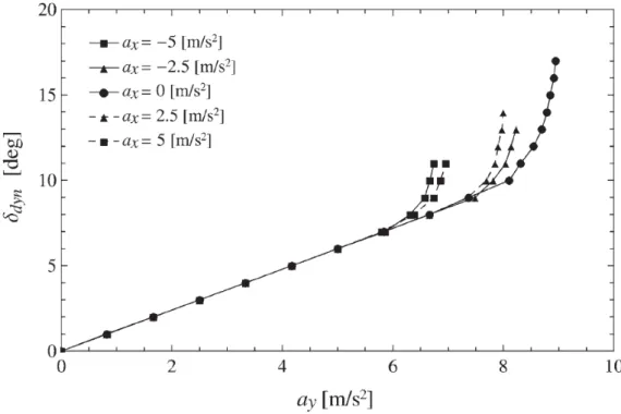
2.3 Understeer characteristic for the vehicle with TV at V =90 km/h and values ofax ranging from−5 to 5 in step of 2.5m/s2(adapted from [2]) . . 79 2.4 Simulation results for a TV application to a FEV with four on-board electric
motors:r-yaw rate,β-sideslip angle,Mz-yaw moment . . . 80 2.5 General scheme of the vehicle demonstrator experimental setup with its
electric drivelines (adapted from [3,4]) . . . 82
2.6 Vehicle Dynamics Area (VDA) of Lommel (BE) proving ground with the vehicle demonstrator . . . 83
2.7 Simplified schematic of the vehicle control structure . . . 85
2.8 Definition of Normal mode, Sport mode and Enhanced Sport mode under-steer characteristics versus passive vehicle experimental data forax =0 and high friction condition . . . 87
2.9 ay,l i n and ay,max maximum values that can be selected for the desired understeer characteristic for high friction condition andV =100 km/h . . 90
2.10 reference yaw rate maprLU T(δ,V,ax,µ) for a high friction coefficient and
2.11 Reference yaw rate correction mechanism . . . 93
2.12 Gain scheduled controllerL(v) . . . 97
2.13 Time history of the disturbance contributions during a sequence of step steers at 90 km/h . . . 102
2.14 Yaw rate and sideslip angle for a step steer maneuver of 100 deg at 100 km/h for the passive and active vehicles . . . 104
2.15 Yaw moment for a step steer maneuver of 100 deg at 100 km/h for LQR and ISM control strategies . . . 104
2.16 Conventionals, integralzand finalssliding variables during ISM control activation . . . 105
2.17r(t) for the passive and active (ISM control with only yaw rate control and concurrent yaw rate and sideslip control) vehicles during sequences of step steers in low tire-road friction conditions with different sideslip thresholds 106
2.18β(t) for the passive and active (ISM control with only yaw rate control and concurrent yaw rate and sideslip control) vehicles during sequences of step steers in low tire-road friction conditions with different sideslip thresholds 106
2.19 Examples of experimental understeer characteristics for the passive and active vehicles . . . 107
2.20r(t) during a step steer for the passive (a) and active (LQR (b), LQR+FF (c) and ISM (d)) vehicles . . . 109
2.21 Mz,sat(t) during a step steer for the LQR, LQR + FF and ISM controls . . . . 110 2.22 ISM yaw moment contributions during a step steer . . . 110
2.23r(t) during a step steer with the ISM control for different values ofωF . . . 111
2.24β(t) during step steers with the ISM control in Enhanced Sport mode, with and without the sideslip angle controller (for different sideslip thresholds, -7 deg, -14 deg, and -21 deg) . . . 112
2.25r(t) during step steers with the ISM control in Enhanced Sport mode, with and without the sideslip angle controller (for different sideslip thresholds, -7 deg, -14 deg, and -21 deg) . . . 113
2.26r(t) andβ(t) for the passive and active (ISM control, Normal mode) vehi-cles during sequences of step steers with a sideslip threshold of 15 deg . . 114
2.28 δ(t),r(t) andβ(t) for the passive and active (in Normal mode) vehicles
during an obstacle avoidance maneuver from an initialV =51.5 km/h . . 115
2.29 Distribution of the successful (indicated by the blank symbols) and unsuc-cessful indicated by ’x’) tests for the passive and active vehicles (in Normal mode), during obstacle avoidance maneuvers . . . 115
2.30 Extended Kalman Filter iterative scheme . . . 118
2.31 Vehicle speedV, torque vectoring yaw momentMz,T V and steering wheel angleδduring a step steer maneuver of 100 deg steering angle at 100 km/h executed in sport mode . . . 122
2.32 Vehicle yaw rater, lateral accelerationay and longitudinal acceleration ax during a step steer maneuver of 100 deg steering angle at 100 km/h executed in sport mode . . . 123
2.33 Experimental and estimate of sideslip angleβfor different selection of matrixRelements . . . 123
2.34 Experimental and estimate of sideslip angleβduring a step steer maneuver of 100 deg steering angle at 100 km/h executed in enhanced sport mode . 124 3.1 General scheme of a DCT with two secondary shafts architecture and power flow representation . . . 131
3.2 Gear Impact . . . 132
3.3 Tip-out maneuver: engine & clutches torques . . . 134
3.4 Tip-out maneuver: vehicle and transmission speeds . . . 134
3.5 Tip-out maneuver: Angular Position Differences ∆ϑ; I: First gears - II: Second gears - FD: Final Drive gears - Diff: Differential gears . . . 136
3.6 Speed-bump maneuver: disturbance longitudinal acceleration and speed 137 3.7 Speed-bump maneuver: vehicle and transmission speeds . . . 138
3.8 Speed-bump maneuver: angular position differences∆ϑ; I: First gears - II: Second gears - FD: Final Drive gears - Diff: Differential gears . . . 139
3.9 Controller Strategy for Noises Reduction . . . 140
3.10 Tip-out maneuver: Torques applied to the Transmission . . . 141
3.12 Tip-out maneuver: ∆ϑon the engaged shaft for active and passive con-figurations; I: First gears - II: Second gears - FD: Final Drive gears - Diff: Differential gears . . . 142
3.13 Tip-out maneuver: ∆ϑon the preselected shaft for active and passive configurations; I: First gears - II: Second gears - FD: Final Drive gears . . . 143
3.14 Tip-out maneuver:∆ϑfor Brake Intervention with and without K2 clutch slip control; I: First gears - II: Second gears - FD: Final Drive gears . . . 143
3.15 Speed-Bump maneuver: vehicle speed for passive and active configurations144
3.16 Speed-Bump maneuver:∆ϑon the engaged shaft for active and passive configurations; I: First gears - II: Second gears - FD: Final Drive gears - Diff: Differential gears . . . 145
3.17 Speed-Bump maneuver:∆ϑon the preselected shaft for active and passive configurations; I: First gears - II: Second gears - FD: Final Drive gears . . . 145
3.18 Speed-Bump maneuver:∆ϑfor brake intervention with and without K2 clutch slip control; I: First gears - II: Second gears - FD: Final Drive gears . 146
3.19 HIL Test Rig 1-TMC 2-customized ESC 3-Brake caliper 4-Brake disk 5-oil tank 6-Data Acquisition System 7-Relay Box . . . 148
3.20 Representation of ABS/ESC hydraulic circuit with input (red) and output (green) . . . 149
3.21 Influence of Bulk modulus on brake pressure trend: experimental (solid black line) vs simulation with constantβ(dotted gray line) and with non-linearβ(dashed gray line) . . . 154
3.22 ’Raising phase’: 1= 1◦chamber TMC, 2= 2◦chamber TMC, b= Rear Right caliper, FL= Front Left caliper, eq= equivalent Front Right+Rear Left caliper, exp=experimental, sim= simulation . . . 155
3.23 Sensitivity analysis on b2 and Ff2: 1= 1stTMC chamber, 2= 2nd TMC
chamber, b= Rear Right caliper, n = nominal condition . . . 155
3.24 ’Falling phase’: 1= 1st TMC chamber, 2= 2ndTMC chamber, b= Rear Right caliper, a= accumulator, exp=experimental, sim= simulation . . . 156
3.25 Effect of PWM Duty Cycle on pressure trend in the brake caliper: the inlet valve is controlled via a constant frequency and variable Duty Cycle . . . . 156
3.26 Raising and falling phases by applying a PWM signal of 40% DC and modu-lation frequency of 900 Hz to the inlet valve and a PWM signal of 25% DC on 50 Hz to the outlet valve . . . 157
3.27 Static GainGsfor both inlet (left) and outlet (right) valve . . . 158 3.28 Experimental validation of non-linear model during ABS emergency
brak-ing under extremely low road friction conditions: b= Rear Right caliper, exp=experimental, sim= simulation . . . 159
3.29 Experimental Validation of Non-Linear Model under a PWM signal excita-tion: b= Rear Right caliper, exp=experimental, sim= simulation . . . 159
3.30 Hydraulic scheme for the raising and falling phase in a brake caliper in-cluding Inlet/Outlet valves, Motor-pump and Spring accumulator. . . 161
3.31 Data Acquisition with a sample time of 0.1 ms of TMC (pT) and Brake (pb) pressures . . . 163
3.32 PWM signal with different frequencies for both Inlet (DC=30%) and Outlet Valves (DC=70%),pb= Brake Pressure . . . 164 3.33 PWM frequency influence on brake pressure ripple for both Inlet (blue)
and Outlet (green) valves . . . 165
3.34 Brake pressure (up) and its gradient (down) vs time for different values of DC (Inlet valve) . . . 165
3.35 Inlet Open-Loop map: pressure gradient vs pressure drop across Inlet valve for different value of DC . . . 166
3.36 Outlet Open-Loop map: pressure gradient vs pressure drop across Outlet valve for different value of DC . . . 167
3.37 Conversion from open-loop map (left) to inverse map (right) for different values of pressure drop across Inlet valve . . . 170
3.38 Inlet Inverse map: DC vs reference pressure gradient and pressure drop across Inlet valve . . . 170
3.39 Outlet Inverse map: DC vs reference pressure gradient and pressure drop across Outlet valve . . . 170
3.40 Block diagram of FF + PI control strategy . . . 171
3.41 Bode plots for transfer functions ne(s)
b(s) (left) and e(s)
3.42 System response to a sequence of step changes of the reference pressure
(dashed gray) . . . 174
3.43 System response to a triangle wave reference pressure (dashed gray) . . . . 175
3.44 System response to a trapezoidal wave reference pressure (dashed gray) . 175 3.45 Transmission Test Rig at Politecnico di Torino . . . 176
3.46 Transmission test bench layout. M1, M2: electric motors; EM1, EM2, ED: speed sensors (encoders); T1, T2,TH S: torque sensors; B: disk (D) brake; SA1, SA2: half shafts. . . 178
3.47 Example of HIL configuration for longitudinal dynamics analysis. . . 179
3.48 DCT Test Rig: zoom on the brake caliper mounting . . . 180
3.49 Speed-Bump crossing: M1 - torque applied by 37 kW motor; M2 - torque applied by 11 kW motor; HS - Half shaft torque . . . 181
3.50 Speed-Bump crossing: transmission and motor speeds . . . 182
3.51 Speed-Bump crossing:∆ϑon the engaged and preselected shafts . . . 182
3.52 Speed-Bump crossing:∆ϑinside the differential . . . 183
3.53 Speed-Bump crossing with different braking pressures: M1 - torque applied by 37 kW motor; M2 - torque applied by 11 kW motor; HS - Half shaft torque183 3.54 Speed-Bump crossing with different braking pressures:∆ϑon the engaged and preselected shafts . . . 184
3.55 Tip-Out Maneuver with and without the control action (brake pressure of 8 bar): M1 - torque applied by 37 kW motor; M2 - torque applied by 11 kW motor; HS - Half shaft torque . . . 185
3.56 Tip-Out Maneuver without (a) and with (b) the control action (brake pres-sure of 8 bar): transmission speeds . . . 185
3.57 Tip-Out Maneuver without (a) and with (b) the control action (brake pres-sure of 8 bar):∆ϑon the engaged and preselected shafts . . . 186
1.1 Model parameters for the single-track model of autonomous vehicle . . . 15
1.2 Root Mean Square of lateral deviationyduring Close-Loop path tracking control . . . 70
2.1 Main I/O signals for TV controller in the dSPACE®AutoBox system with their discretization times and their availability on vehicle CAN network (Yes:present, No:absent) . . . 82
2.2 Reference yaw rate correction∆rr e f . . . 92 2.3 Performance indicators for the step steer test for the passive and controlled
vehicles . . . 109
2.4 Performance indicators for the step steers for different values ofωF . . . . 111
Autonomous Steering Control
1.1 Introduction on Autonomous Steering Driving
AutonomousorSelf-Drivingvehicles are nowadays a hot-topic for research and develop-ment in both industrial and academic fields, also arousing interest among social and governmental communities, well beyond the automotive engineering. ’Autonomous driving’ represents a generic term for identifying a non conventional vehicle that is able to drive in urban and/or highway scenarios without or with a partial human interven-tion. In order to provide a common terminology, in [5] are considered different levels of driving automation fromno automationin ’level 0’ tofull automationin ’level 5’: the automated driving is distinguished from human driving if specific systems are designed to monitor the driving environment. Each level deals with the execution of steering and acceleration/deceleration tasks, the monitoring of driving environment, the fallback of dynamic driving task and the system capability. An example of self-driving application, with current technologies available on automotive market, is the Conventional Cruise Control (CCC) designed for keeping constant a desired vehicle speed set up by the driver; the ’autonomous’ system takes full control of throttle and brake command in order to track the reference speed but with no environment monitoring so that the driver is responsible for control overtaking in emergency situations. This simple technology is now popular enough to be accepted by drivers and its safety benefits/limits have been studied by several authors [6,7]. An advanced version of CCC is the Adaptive Cruise Control (ACC) [8–11] which elaborates the information coming from specific RADAR for obstacle detection thus enhancing the communication with external environment and providing a warning feedback to the driver which is expected to react in collision risk situations. In the case of Automatic Emergency Braking (AEB) [12,13], the system is also requested to provide a braking intervention for obstacle avoidance purposes. For
autonomous driving applications, three different layers can be identified as indicated by [14,15]:
• TheStrategiclayer, for gathering information from the environment surrounding the vehicle, i.e. pedestrian or obstacle recognition, lane and road signals identifi-cation;
• TheTacticallayer, for providing the reference signals for the next layer, i.e. refer-ence path to be followed or referrefer-ence speed to be reached;
• TheControllayer, for evaluating the commands for each autonomous or automatic vehicle components and tracking the reference behavior imposed by the Tactical layer;
The present chapter is focused on the analysis and the development of the Control layer in the specific application of an automatic steering control for path tracking and obstacle collision avoidance purposes. The path tracking control is a well-known topic in the robotic control field [16–18] and driver modeling [19–21]. Several experiments were carried out for automatic driving [22,23] where the reference path is generally provided through inductive cables or magnetic markers, but new technologies about Global Positioning Systems (GPS) have incremented the position accuracy through the use of external global navigation satellite system (GNSS). Different feedback controllers have been designed for automated path tracking control (an extended review is described by [24]) and they can be generally divided into two separate categories.
The first category includes all methods based on simple geometrical relationships by exploiting the vehicle kinematic models (i.e. by approximating a zero slip angle for the front and rear tires) described by the well-known Ackerman steering formula. One example is thePure Pursuitalgorithm whose objective is to calculate the curvature of the arc from the vehicle position to the desired position placed at alook-aheaddistance on the reference path [25, 26]; a different geometric-based approach is designed by Stanford’s University during the DARPA Grand Challenge [27], usually referred asStanley method, which elaborates the steering angle as a combination of vehicle yaw angle error and a term based on the lateral deviation of the front axle with respect to the reference path.
The second category deals with all feedback controllers based on the simplified linear single-track model, described in section1.3, that takes into account a different slip angle for the front and rear axles and provides a second order yaw dynamics with damping and stiffness coefficients variable with vehicle speed. The Proportional Integral Derivative (PID) is the most used control logic adopted for steering angle evaluation: a PD structure
on lateral deviation error added to a P control on heading error is designed by [28] which proves that yaw angle error contribution further improves the tracking performance, as it is also confirmed by [29] where only the lateral position error is taken into account with evident worse results. A more detailed analysis is conducted by [30] based on frequency responses of lateral acceleration and yaw rate with respect steering angle, calculated from the linear single-track model: the effect of the vehicle speed and friction coefficient is studied and consequently a feedforward steering contribution based on reference path curvature is coupled with a feedback yaw rate and lateral acceleration control. Moreover, it is suggested to design the look-ahead distance as an increasing function of vehicle speed. The benefits introduced by a feedforward contribution which avoid the selection of high feedback control gain is shown by [31] thus also demonstrating its importance in terms of tradeoff between stability and tracking performances. In [32] a PIDD2controller is designed, according to the parameter state approach [33], for the path tracking problem related to an automated bus in order to be robust with respect to the variation of vehicle speed and mass in a specific range. The same state parameter approach is used for autonomous passenger vehicle by [34,35]. The classical loop-shaping theory is applied in [36] where two different controllers are proposed for achieving alternatively a better ride comfort or a good tracking performance. Linear Quadratic Regulator (LQR) based on optimal control theory is applied by Nissan [29] which makes a comparison against the PD strategy with the final conclusion that the LQR logic is ” unable to track the path accurately on curves” due to large model error on the curvature part of reference path. This issue is solved with an additional feedforward (FF) contribution to the LQR control in [9]. A non conventional LQR design is presented in [37–39] for the PATH framework: authors adopt the loop shaping technique for achieving the robustness on measurement noise at high frequencies and introduce a performance index that takes into account the ride quality. Thecenters of percussionconcept is shown by [40] for a four-wheel-steering (4WS) through the design of a first order sliding model control meanwhile [41] has implemented a super-twisting version for reducing the chattering problem. More references in the filed of sliding mode theory and application are [42–45]. Other controller structures has been analyzed and implemented: H∞in [46,47], back-stepping control [48] and fuzzy logics [49]. Recently, the path tracking control strategies are further improved for being robust at high lateral accelerations [50–52] even with the implementation of model predictive controls now extensively used in simulation and preliminary experimental tests [53–55].
Similar to the difference between CCC and ACC, the path tracking problem can be extended to an Obstacle Collision Avoidance (OCA) algorithm where the reference path is no more fixed but it is changed in real-time by elaborating further information coming from other sensors (Radar, Lidar, Camera) thus enabling the communication
with external environment. The core aspect of OCA control logic is represented by the path planning algorithm that needs to provide the reference path for the lower controller layer (i.e. path tracking control). A 3D virtual dangerous potential field is used for generating the desired trajectory to avoid obstacle in real-time and a Multi-constrained Model Predictive Control (MMPC) problem is formulated in [56]. In [57] a novel algorithm for obstacle avoidance path planning, defined asnavigation circle, is developed and optimized to provide feasible trajectories in real-time. A decision-making algorithm is presented in [58] where a group of path candidates are generated starting from a global reference path and the local reference trajectory is selected according to safety, smoothness and consistency criteria in presence of static obstacles. The path planning has been experimentally tested during the 2010 Autonomous Vehicle Competition. In 1993 authors from Stanford University [59] proposed for the first time theElastic Bands theory for deforming an initial reference path into a collision-free path which is able to take into account the presence of local obstacles. The same OCA method is applied by [60] with modifications to road vehicle based systems and realistic simulation results are presented using high fidelity vehicle models with several different collision scenarios.
The intent of the present section is to design an automatic steering control for an autonomous vehicle equipped with Electric Power Assist Steering (EPAS) and drive-by-wire technologies. Despite the importance of tires lateral force in path tracking controller, the single-track model is chosen instead of a kinematic/geometric one ([25– 27]) and it is further enhanced by introducing the steering actuation (EPAS) dynamics if compared with existing literature.The steering action is calculated to let the vehicle follow a reference path which is stored in a Digital Map properly built to be available in real-time. Furthermore, the contribution described in the following chapter is the enhancement of a Proportional + Derivative (PD) control designed with the Parameter State Approach [33, 35] (PSA) by coupling it with a static Feedforward (FF) or with an integral sliding mode (ISM) for improving the tracking performance in cornering maneuvers:the FF term requires the knowledge of the instantaneous reference path curvature, meanwhile the ISM can be designed to reject external disturbances without the exact evaluation of the path curvature. Experimental tests are carried out for showing and comparing the efficacy of the two controllers against PD control and manual driving behavior. Moreover, an experimental implementation of an obstacle collision avoidance system based on the elastic band method is briefly described with the main objective to show that the method can be implemented in real time and used in actual vehicles.
The present chapter is divided into five sections by including the present introduction and the conclusion: section 2 shows the autonomous vehicle demonstrator with its
set-up; in section 3 the single-track model with steering dynamics is presented; section 4 is focused on path tracking control design and its implementation for an OCA application which are finally experimentally verified with specific tests in a proving ground.
1.2 Experimental Setup of the Autonomous Vehicle
The vehicle demonstrator, shown in Fig.1.1, used for dynamics model validation and con-trol calibration is a Ford Fusion hybrid which has been converted into an autonomous vehicle through the installation of EPAS module, throttle-by-wire and brake-by-wire Dataspeed interfaces. Power Distribution MicroAutobox II GPS/IMU LIDAR RADAR CAMERA Drive-by-wire HMI Control GPS Antenna
Figure 1.1 Vehicle Demonstrator and Sensors/Actuators Platform
The Dataspeed Inc. [61] EPAS module and Throttle-Brake Combination By-Wire in-terfaces enable computer control of the steering wheel, the throttle and braking systems in a safe and effective manner. This plug-in ready kit requires no modification to the factory harnessing and can be installed in few minutes. Industry standard CAN and USB networks enable control and monitoring of the steering wheel (angular position), the throttle and braking systems (pedal positions). The Dataspeed modules are connected through CAN bus communication to a dSPACE®MicroAutoBox II electronic unit where controller logic, previously designed in Matlab®/Simulink®environment, is flashed. A range of several sensors are installed on-board vehicle in order to monitoring the external environment and to localizing vehicle position:
• Delphi ESR [62] radar combines a wide field of view at mid-range with long-range coverage to provide two measurement modes simultaneously. Based on
Simulta-neous Transmit and Receive Pulse Doppler (STAR PD) Waveform technology, the ESR provides independent measurements of range and range-rate and superior detection of clustered stationary objects. Mid-range coverage not only allows vehicles cutting in from adjacent lanes to be detected but also identifies vehicles and pedestrians across the width of the equipped vehicle. Long-range coverage provides accurate range and speed data with powerful object discrimination that can identify up to 64 targets in the vehicle’s path.
• Velodyne VLP-16 Lidar [63] creates 360°3D images by using 16 laser/detector pairs mounted in a compact housing. The housing rapidly spins to scan the surrounding environment and the lasers fire thousands of times per second, providing a rich, 3D point cloud in real time. Advanced digital signal processing and waveform analysis provide high accuracy, extended distance sensing, and calibrated reflectivity data. • Mobileye camera 5 [64] uses a smart digital camera located on the front windshield
inside the vehicle. Inside the camera, Mobileye’s powerful EyeQ2® Image Pro-cessing Chip provides high-performance real-time image proPro-cessing, by utilizing the Mobileye vehicle, lane and pedestrian detection technologies to effectively measure and calculate dynamic distances between the vehicle and road objects. • OXTS xNAV 550 RTK GPS [65] integrates dual L1/L2 GNSS receivers for 2 cm RTK
position accuracy and an Inertial Measurement Unit (IMU) with three accelerom-eters and three angular rate sensors used to smooth the jumps in GNSS and fill in missing data. The improved receivers also mean better heading accuracy. Its communication with MicroAutoBox II is via UDP protocol.
In the present activity, the differential OXTS GPS is the only sensor used for vehicle position localization as feedback input to the path tracking controller meanwhile other sensors are going to be integrated for real-time implementation of obstacle collision avoidance control logic according to which is generally referred asSensor-Fusion tech-nology.
The vehicle demonstrator architecture is also equipped with a power distribution unit for managing the electric energy between vehicle high voltage battery and sen-sors/actuators.
Finally, A Human Machine Interface (HMI) with touch screen technology provides a control panel for basic command selections (power on/off all devices and switch between manual and autonomous modes).
1.3 Single-Track Model
The present section describes a linearized single-track model used for designing con-troller strategies that are introduced in next sections. This linear model (see [66,67] for further details) is also able to describe vehicle dynamics for a lateral acceleration up to 4m/s2. The vehicle is considered symmetric with respect its longitudinal direction so that the front and the rear axles can be represented by single wheels as indicated in Fig.1.2where an inertial reference systemOE,XE,YE,ZE and a vehicle reference system
O,x,y,zare shown.
Figure 1.2 Single-Track Model (adapted from [1])
When vehicle speed is very small, and slip angles can be neglected (ideal kinematic steering), all points of vehicle move along a circle with the center of the curvature being
KA which coincides with the instantaneous center of rotationM of the motion. The steering angle required to execute this motion is given as:
tanδw=q l R2M−b2 |δw|≪1,b≪RM → δw≈ l RM (1.1)
In a real scenario, slip angles cannot be neglected and the new instantaneous center of rotation is evaluated from the front and rear wheel speed directions. The following assumptions are considered for evaluating the single-track model equations:
• the vehicle is assumed as a rigid body in motion on a 2D plane with massmand inertia momentJz
• vehicle speedV is assumed constant and only two degree of freedom (yaw rate
r=ψ˙and sideslip angleβ) are taken into account
• vehicle sisdeslip angleβ, tires slip anglesαi and yaw rate acceleration ˙r are con-sidered small enough to consider the linear part of vehicle dynamics
• Front steering action (small wheel steering anglesδw)
1.3.1 Dynamics equations
A rigid body in motion on a 2D surface can be described by 3 degrees of freedom: global reference positionsXE,YE of vehicle center of gravity and its yaw angleψ.
mX¨E =FX mY¨E =FY Jzψ¨ =MZ (1.2)
whereFX,FY andMZ are the total forces applied alongXE,YE axes and total yaw mo-ment aroundZE axis. In order to have a linearized vehicle model and avoid trigonometric expression ofψ, Eq.1.2can be expressed in the vehicle reference frame:
dV⃗ d t ¯ ¯ ¯ ¯ ¯ E = dV⃗ d t ¯ ¯ ¯ ¯ ¯ v +⃗ω∧V⃗ = ˙ u ˙ v 0 + −r v r u 0 (1.3) m( ˙u−r v) =Fx m( ˙v+r u) =Fy Jzr˙ =Mz (1.4)
whereuandv are the vehicle speed components respectively alongxand yaxis and
Fx,Fy,Mzare the same of Eq.1.2but expressed in the vehicle reference frame. Eq.1.4 are non-linear with respectu,v, andr but, since the sideslip angleβis supposed to be
small, it is possible to linearize the trigonometric functions: u =Vcos(β)≈V v =Vsin(β)≈Vβ (1.5)
thus leading to:
m( ˙V−r Vβ) =Fx m(Vβ˙+βV˙+r V) =Fy Jzr˙ =Mz (1.6)
If the interaction between longitudinal and lateral tire forces is neglected, the first equation of system1.6can be decoupled from the remaining two, thus reducing the degrees of freedom to the sideslip angleβand yaw rater. Furthermore, if the speedV is considered constant the system1.6can be reduced to:
mV( ˙β+r) =Fy Jzr˙ =Mz (1.7)
Fy andMz can be related to tires forces:
Fy =P∀iFxisin(δi)+ P ∀iFyicos(δi)≈ P ∀iFxiδi+ P ∀iFyi Mz =P∀iFxisin(δi)xi+ P ∀iFyicos(δi)xi≈ P ∀iFxiδixi+ P ∀iFyixi (1.8)
whereFxi, Fyi are force components onit h axle andxi, yi are the coordinates of its center. In Eq. 1.8, drug forces and self-alignment yaw moments are neglected and trigonometric functions are linearized by considering low values of wheel steering angles δi. Furthermore, the productsFxiδi can be also neglected since they are negligible with respect other terms of Eq.1.8. Tires lateral forcesFyi depends on several variables such us tires slip angles, tires vertical forces, road contact friction coefficients and tires slip ratio. In order to have a linearized model,Fyi can be evaluated as:
Fyi =Ciαi (1.9)
whereCi is the cornering stiffness ofit haxle and not of an individual wheel: with the single-track model the vehicle is assumed as a rigid body (roll angle neglected) thus compensating the camber forces between right and left wheels. Moreover, even the toe angle influence and lateral load transfer are neglected: this would be correct if a linear relation occurs between cornering stiffness and load transfer since the increase of the cornering stiffens of the most heavily loaded wheel is exactly compensated by the
decreasing of the cornering stiffness of the opposite wheel; This is not generally verified and the load transfer introduces a reduction of axles cornering stiffness eve though this effect is negligible for a lateral acceleration lower than 5m/s2. Furthermore, a positive toe angle increases axle cornering stiffness meanwhile a negative value decreases it.
Tires slip angles can be expressed as a function of their correspondent wheel speeds as indicated in Fig.1.3. The speedVi of theit hwheel centerPi can be referred to the
Figure 1.3 Kinematic diagram of wheel speed (adapted from [1])
speed of vehicle center of gravityV:
⃗ VPi =V⃗G+ψ˙∧(Pi⃗−G)= ( u−ψ˙yi v+ψ˙xi ) (1.10)
The angleβi between the direction ofV⃗Pi and vehicle x axis is defined as: βi=ar c t an(vi
ui
)=ar c t an(v+ψ˙xi
u−ψ˙yi
) (1.11)
If theit htire is rotated by a steering angle ofδi, its slip angle is: αi=δi−βi=δi−ar c t an(v+ψ˙xi
u−ψ˙yi
Eq. 1.12can be easily linearized by considering that the term ˙ψyi is negligible with respect vehicle speedV:
αi=δi−βi ≈δi−ar c t an(v+r xi
V )=δi−β− xi
V r (1.13)
In the linearized expression ofαi, the coordinateyi doesn’t appear with the consequence that ifδi is the same between right and left wheels also their slip angles are equal as highlighted in Eq.1.13: this allows to approximate vehicle dynamics with a single track scheme (1.2) thus writing equations in terms of axle instead of single wheels.
Finally, slip angles of front and rear axles are reported respectively in the following equations: αF =δF−β−Var αR =δR−β+Vbr (1.14) In most of passenger cars, and even in the vehicle considered in this activity, only the front axle can be steered so that the assumption δR =0 can be used without loss of generality.
The final equation of linearized single-track vehicle model are:
mV( ˙β+r) =(−CF−CR)β+(−CVFa+CVRb)r+CFδF Jzr˙ =(−CFa+CRb)β+(−CFa 2 V − CRb2 V )r+(CFa)δF (1.15)
It is a system of two first order differential equations in terms ofβandr even though these two variables are dimensionally an angular speed (r) and something related to vehicle speed (β) thus implying that their derivative are accelerations. The steering angle δF can be considered an input for the system.
1.3.2 Steady-State behavior
In steady-state conditions ( ˙β=0 and ˙r=0), vehicle trajectory is circular with a constant radius equal to:
R=V r (1.16)
From Eq.1.15, the evaluation of steady-state values of sideslip angleβand yaw rater
deals to: β = CFCRbL−mV2CFa CFCRL2+mV2(bCR−aCF)δF r = CFCRLV CFCRL2+mV2(bCR−aCF)δF (1.17)
whereL =a+b is the vehicle wheelbase. The new parameter named as Understeer gradientcan be defined as:
K =m L( b CF − a CR ) (1.18)
so that the following steady-state gains are formulated: • Sideslip angle steady-state gain
β δF =(1− maV2 bLCR ) b L+K V2 (1.19)
• Yaw rate steady-state gain
r
δF =
V
L+K V2 (1.20)
• Lateral acceleration steady-state gain
ay δF =
V2
L+K V2 (1.21)
• Curvature steady-state gain
ρ δF =
1
L+K V2 (1.22)
Eq.1.1indicates that the curvature steady-state gain in kinematic condition (Eq.1.1
with assumption of slip angles negligible) can be corrected by a factor of L+K VL 2 to take into account the important influence of wheel slip angles. If the understeer gradient is null the value of R1δ is constant and vehicle response to any steering angle is equal to that one in kinematic condition; This doesn’t mean that the vehicle is operating in kinematic condition, since wheel slip angles are not negligible so that its behavior is generally defined as ’neutral condition’.
If K >0, the value of R1δ decreases with vehicle speed: for keeping constant the trajectory radius, the steering angle has to be increase when vehicle speed increases. The vehicle is operating in ’understeer condition’. A direct measure of vehicle understeer behavior is the ’characteristic velocity’, defined as the speed at which the steering angle required to follow a desired trajectory is double the Ackerman angle by means the curvature steady-state gain is equal to 1/2L:
Vc ar =
r
1
IfK<0, the value of R1δ increases with vehicle speed until it reaches the values of the ’critical velocity’: Vcr i= r 1 −K (1.24)
where vehicle response tends to infinity and the vehicle becomes unstable. A vehicle that presents such a behavior is operating in ’oversteer condition’: for this configuration the critical velocity must be greater than the vehicle max speed.
The value of sideslip angle steady-state gainβ/δF decreases when speed increases until it becomes null for the velocity:
Vβ=0=
s
bLCR
am (1.25)
For higher vehicle speeds its value becomes negative and tends to infinity when speed tends to critical velocity for an oversteer condition; In case of understeer condition its value tends to:
β δF =
aCF
aCF−bCR
(1.26) In case of neutral condition, the slip angles of front and rear axles are equals. For oversteering vehicles, slip angle of rear axle is higher (in absolute value) than the front axle one meanwhile the opposite situation occurs for understeering vehicles. Fig.1.4
shows a graphic description of vehicle behavior during different conditions. The vehicle presents a front steering axle A and a fixed rear axle B. For low values of vehicle speed, the kinematic condition is almost verified: the slip angles are null and the trajectory center is placed in O. In the conditionαF =αRthe angle BO’A is still equal toδF and the point O’ leads on the same circle identified by points A, B and O: the vehicle is operating in neutral condition. If|αF| > |αR|the curvature center is moved to point O” and radius R” is higher than R thus leading to and understeering behavior. If|αF| < |αR|the curvature center is O”’ and the radius R”’ is lower than R thus leading to an oversteering behavior. These considerations are verified only if the understeer gradientK is constant and doesn’t depends on vehicle speed; in a real scenario, the value ofK is influenced by vehicle speed that can modify its understeering behavior.
1.3.3 Experimental Validation
The present section aims to describe the single-track model and to validate it with experimental test carried out with the prototypal vehicle equipped with drive-by-wire technology. Most of the single-track model parameters (m,Jz,a andb) are obtained
Figure 1.4 Lateral behavior of a vehicle with a single steering axle (adapted from [1])
through specific measurements on the vehicle meanwhile the front and rear cornering stiffness values are evaluated and proper tuned in order to get the best fit between model and experimental data. All single-track parameters are reported in Table1.1. Three specific experimental test are here presented in order to show the efficacy and limits of a single-track model:
1. Ramp steer at constant speed 2. Step steer at constant speed 3. Skid pad
Table 1.1 Model parameters for the single-track model of autonomous vehicle
Symbol Description Value
m Vehicle mass with 4 passengers 1997.6kg Jz Inertia moment around vehicle z axle 3728kg m2
a Front semi-wheelbase 1.3008m
b Rear semi-wheelbase 1.5453m
L Wheelbase 2.84607m
CF Front Cornering Stiffness 1.3e5N/r ad
CR Rear Cornering Stiffness 15.9e5N/r ad
Rs Steering ratio 14.6
ls Preview Distance 0.5m
[n2n1n0] Numerator of steering dynamics [74.45 −1001 53760]
[d4d3d2d1d0] Denominator of steering dynamics [1 36.33 1205 12950 53760]
All these maneuvers are executed on a flat surface (no bank angle) and in high friction conditions. The single-track model receives as input the experimental steering angle measured during each test in order to have coherent comparison.
Ramp steer at constant speed
The ramp steer maneuver can be described with the following steps: • set the cruise control at a specific speed
• when the desired speed is reached, the steering angle is gradually increased from 0 to 400 deg with a slope of 14 deg/s
• the vehicle is stopped when lateral acceleration saturates
These steps can be identified in Fig.1.5where input steering angle and speed are shown. The vehicle speed can be considered constantly equal to 30km/hfor the whole applica-tion of the ramp steering acapplica-tion. The variables analyzed during the maneuvers are the sideslip angleβ, the yaw rater(output of single-track model) and the lateral acceleration
ay reported in Fig.1.6. This test is useful to observe the quasi-static lateral behavior of the vehicle in the whole range of lateral acceleration thus allowing to validate the single-track model in the linear part of vehicle dynamics and to detect the limit beyond which the model is not enough accurate to describe tires forces saturation. It is possible
0 5 10 15 20 25 30 35 40 -200
0 200 400
Steering Angle [deg]
0 5 10 15 20 25 30 35 40 0 20 40 Vehicle Speed [km/h] Single-Track model Experimental
Figure 1.5 Ramp steer maneuver: steering angle and vehicle speed
0 5 10 15 20 25 30 35 40 0 5 10 a Y [m/s 2 ] Single-Track model Experimental 0 5 10 15 20 25 30 35 40 0 50 100 r [deg/s] Single-Track model Experimental 0 5 10 15 20 25 30 35 40 Time [s] 0 5 10 β [deg] Single-Track model Experimental
Figure 1.6 Ramp steer maneuver: sideslip angleβ, yaw rater=dψ/d tand lateral accelerationay
to appreciate that the linear single-track model is able to give a good matching with respect experimental values for lateral acceleration up to 5 m/s2.
Step steer at constant speed
The step steer maneuver can be described with the following steps: • set the cruise control at a specific speed
• when the desired speed is reached, an instantaneous step steering action is applied and kept constant to a desired value
• the vehicle is stopped when the vehicle trajectory is stabilized
Different step steer amplitudes are selected in order to verified the single-track model in different operating conditions, as indicated in Fig.1.7. All the tests are executed by using
0 0.5 1 1.5 2 2.5 3 Time [s] 0 20 40 60 80 100 120
Steering Angle [deg]
Current Reference
Figure 1.7 Step steer maneuver: reference and current steering angle for different amplitudes
the cruise control to keep the speed equal to 30km/h. Fig.1.7also shows the comparison between the steering angle set for the EPAS system and its response: the dynamics of the steering reaction must be taken into account and a model will be proposed in next section. Step steer test are usually adopted for analyzing the transient vehicle behavior
Figure 1.8 Step steer maneuver: sideslip angleβ, yaw rater=dψ/d tand lateral accelerationay from experimental test (EXP) and single-track model (STM)
values of lateral accelerationay, yaw rater and sideslip angleβare well described by the single-track model meanwhile the transient response ofay seems to be different from experimental data: this aspect is related to the hypothesis of single-track model according which ˙β<<rthus leading toay=V(r+β˙) cos(β)≈V r; Since the final purpose of the single-track model is for vehicle position control design, a further experimental validation can be carried out by comparing GPS position. In the single-track model, vehicle global position is evaluated from yaw rate, sideslip angle and speed:
ψ =Rψ0r d t XG = R
X0(V cosβcosψ−V si nβsinψ)d t
YG =
R
Y0(V cosβsinψ+V si nβcosψ)d t
(1.27)
whereXGandYG are the east and north global vehicle coordinate andψthe yaw angle with respect the X axis. Values ofψ0,X0andY0are obtained from experimental data in
order to make the comparison shown in Fig.1.9.
0 50 100 150 X [m] -150 -100 -50 0 Y [m] STM EXP 60 deg 40 deg 80 deg 100 deg
Figure 1.9 Step steer maneuver: vehicle position for different steering angles from both experi-mental test (EXP) and single-track model (STM)
Finally, the single-track model here presented is able to catch the linear part of vehicle dynamic for a lateral acceleration up to 5 m/s2and to well predict the vehicle global position.
Skid Pad
The Skid Pad test is generally used to evaluate the understeer/handling characteristic of the vehicle by means the vehicle sensitivity to a steering input. The test consists
of following a reference trajectory with constant radius while the gas pedal is slowly increased up to the max possible value: increasing the vehicle speed and so the lateral acceleration, forces the driver to adjust the steering angle to increase lateral forces for following the desired constant radius path. The reference path here used has a constant radius of 30 m and the most important variable are plotted in Fig.1.10,1.11and1.12.
20 40 60 80 100 120 140 160 180 0 100 200 δ [deg] 20 40 60 80 100 120 140 160 180 0 50 100 Gas [%] 20 40 60 80 100 120 140 160 180 Time [s] 0 50 100 V [km/h]
Figure 1.10 Skid Pad: vehicle steering angleδ, gas pedal and speedV
20 40 60 80 100 120 140 160 180 -1 0 1 a x [m/s 2 ] 20 40 60 80 100 120 140 160 180 -10 0 10 a y [m/s 2 ] 20 40 60 80 100 120 140 160 180 Time [s] -50 0 50 r [deg/s]
Figure 1.11 Skid Pad: vehicle longitudinalax, lateral accelerationay and yaw rater
It is worth noting that the vehicle speed doesn’t overpass 50 km/h even if the gas pedal is further increased as a consequence of the tire forces saturation (also highlighted by lateral acceleration and yaw rate). The handling characteristic can be evaluated based on the driver steering correction with respect the kinematic steering (δF−δK i n) as function of lateral acceleration as shown in Fig.1.13. The upper subplot of Fig.1.13is usually
-20 0 20 40 60 X [m] -50 -40 -30 -20 -10 0 10 Y [m] Path
Figure 1.12 Skid Pad: vehicle GPS position
0 1 2 3 4 5 6 7 8 0 2 4 δ F -δ Kin [deg] Raw Data Robust Fit 0 1 2 3 4 5 6 7 8 a y [m/s 2 ] -2 0 2 4 β [deg] Raw Data Robust Fit K
Figure 1.13 Skid Pad handling characteristics:δF−δK i nandβvsay
adopted for calculating the understeer gradientK defined in Eq.1.18: it is geometrically equal to the slope of its linear part. The value ofK calculated from single-track model by using Eq.1.18is 0.006 rad s2/m: it is sufficient close to the slope of the handling characteristic (0.004 rad s2/m). The sideslip angle decreases with lateral acceleration until it changes its sign and tends to an asymptotic behavior; the speed value at which sideslip angle becomes equal to 0 is 51 km/h which is the same calculated by Eq.1.25
using single-track parameters. It is also evident the saturation in both the subplots: when lateral acceleration increases, the driver correction increases until any driver correction is not sufficient to follow the reference path.
1.3.4 Steering Dynamics Model
Fig.1.7has proved that the dynamic behavior of EPAS system needs to be analyzed and integrated with the single-track model. Due to a lack of knowledge about mechanical and electrical parameters for building a mathematical model, a system identification of steering actuation is carried out since the input (desired steering commandδI n) and output (measured steering angular positionδOut) signals are available in real-time. For a complete and detailed description of it, a sweep frequency test (SFT) is carried out in order to plot the frequency response function (FRF) of the steering actuation. The SFT consists of applying a sinusoidal steering command with a constant amplitude and variable frequency (linear time-variant):
δI n =δ0sin(2πf(t)t) f(t) =f0+ fTT−f0t (1.28)
wheref0is the frequency at initial timet0and fT the frequency at timeT. One exam-ple of sweep frequency test with constant amplitude of 90 deg is shown in Fig.1.14. Under the assumption of uncorrelated noise on the output signal and negligible noise
0 20 40 60 80 100 120 Time [s] -100 -50 0 50 100
Steering Angle [deg]
δ
In
δ
Out
Figure 1.14 Sweep frequency test with constant amplitude of 90
contamination on the input, the so calledH2(f) estimator of FRF can be used:
H2(f)=
Py y(f)
Py x(f)
(1.29)
wherePy y is the auto power spectral density of the output andPy xis the cross power spectral density between output (δOut) and input (δI n). To evaluate the quality of the