Borehole damaging
under thermo‑mechanical loading
in the RN‑15/IDDP‑2 deep well:
towards validation of numerical modeling using
logging images
M. Peter‑Borie
1*, A. Loschetter
1, I. A. Merciu
2, G. Kampfer
2and O. Sigurdsson
3Abstract
A wider exploitation of deep geothermal reservoir requires the development of Enhanced Geothermal System technology. In this context, drilling and stimulation of high‑enthalpy geothermal wells raise technical challenges. Understanding and predicting the rock behavior near a deep geothermal wellbore are decisive to imple‑ ment stimulation strategies to reach the couple temperature/flowrate target. Numeri‑ cal modeling can contribute to enhanced stimulation processes thanks to a better understanding of impact of stress release, pressure changes and rock cooling in the near‑wellbore area. In this paper, we use Discrete Element Method (code PFC2D, © Itasca Consulting Group), and more specifically bonded‑particle model to capture the thermo‑mechanical processes at metric scale. The application case corresponds to the beginning of thermal stimulation at Reykjanes in well RN‑15/IDDP‑2 (Iceland, IDDP‑2 project and H2020 project DEEPEGS). A cold fluid is injected at a depth of 4.5 km where the rock temperature is above 430 °C and the well pressure is around 34 MPa. Since we have site‑specific data and logging images after drilling, we attempt to link the simula‑ tions with the reality. The numerical results are confronted with incipient interpretation of logging images and with analytical solution to go towards validation of the mod‑ eling approach. Numerical results show breakouts and thermally and/or mechanically induced fractures consistent with the analytical solutions. Moreover, the sensitivity analysis on uncertain parameters yields important clues regarding some logging fea‑ tures as, for example, asymmetric damaging or caving.
Keywords: EGS (Enhanced Geothermal System), Borehole, Thermal stimulation, Fracture initiation, DEM (Discrete Element Model), PFC2D, LWD, Borehole logging images
Open Access
© The Author(s) 2018. This article is distributed under the terms of the Creative Commons Attribution 4.0 International License (http://creat iveco mmons .org/licen ses/by/4.0/), which permits unrestricted use, distribution, and reproduction in any medium, provided you give appropriate credit to the original author(s) and the source, provide a link to the Creative Commons license, and indicate if changes were made.
RESEARCH
*Correspondence: m.peter‑[email protected] 1 BRGM, 3 av. C. Guillemin, BP36009, 45060 Orléans Cedex 2, France
Background
EGS (enhanced/engineered geothermal system) constitutes a potential renewable energy technology to produce heat and electricity from geothermal reservoirs deficient in fluid or in permeability. In most cases, reaching an economically viable temperature target requires drilling down to several kilometers depth, where the permeability of the system is generally naturally low. The implementation of stimulation strategies is then neces-sary to increase the injectivity or the productivity of the wells (Tester et al. 2006). The deployment of such EGS method in a wide range of geological contexts is still a tech-nical challenge, and the number of projects in operation is currently limited. Accord-ing to EGEC (2017), concernAccord-ing EGS, three electricity plants (Insheim and Landau in Germany, Soultz-sous-Forêts in France; the reservoir temperatures are, respectively, > 160 °C, 160 °C and > 180 °C; Lu 2018) and one heat plant (Rittershoffen in France, the reservoir temperature is 177 °C; Baujard et al. 2017) are now in operation, with a further ten plants under development.
In this context, the EU-funded H2020 DEEPEGS (Deployment of DEEP Enhanced Geothermal Systems for sustainable energy business) project aims at demonstrating the feasibility of EGS in high-enthalpy reservoirs (temperature up to 550 °C, with an Ice-landic demonstrator) and in deep hydrothermal reservoirs (temperatures around 200 °C, with French demonstrators), to deliver new innovative solutions and models for wider deployments of EGS. The first demonstrator deployed in the frame of the DEEPEGS pro-ject is located in the Reykjanes geothermal system in southwest Iceland. The deepening of the wellbore RN-15 from 2500 m depth (RN-15/IDDP-2) began in August 2016 and the well is completed at a depth of 4659 m MD (measured depth, ~ 4.5 km vertical depth) in January 2017 (temperature around 500–530 °C) (Friðleifsson et al. 2017; Friðleifsson and Elders 2017a, b; Stefanson et al. 2017). RN-15/IDDP-2 provides information about the deep geology and the deep rock behavior in the Icelandic context. Notably, bore-hole images provide a unique view of the geological structure of the Icelandic crust. To improve the productivity of the well (estimated injectivity index around 1.7 L s−1 bar−1 at the end of drilling), stimulations in the form of cold-water injection (mainly thermal stimulations) have been performed to connect the wellbore to existing hydraulic path-ways, i.e., pre-existing natural fracture network.
Understanding all the processes that lead to fracture initiation in the EGS near-wellbore remains challenging due to the high temperatures. In this context, numerical modeling contributes to improve our understanding and it allows for predictions in the future. The objective of this article is to propose a physical modeling approach contrib-uting to the understanding of phenomena occurring in the wellbore vicinity during drill-ing and EGS operations. We focus on the thermo-mechanical processes induced by the rock cooling. The choice of the numerical method is based on assumptions drawn from onsite information. The results are compared with results from analytical equations and with observations made during drilling to critically discuss the numerical results and go towards validation of the chosen approach.
and/or mechanically induced fractures consistent with the analytical solutions and with observations made during drilling. We finish with words of conclusion and with discus-sion on the experienced limitations and perspectives.
Geological knowledge
Regional data
The in situ geological, mechanical and thermal conditions are little known in the deep part of the Reykjanes field. The deepest well in this area was shallower than 3 km before drilling the IDDP-2 well. Besides, geophysical methods are limited for investigations at several kilometers depth. We summarize below the information concerning the regional geology, the regional stress state and the rock behavior.
Geology
The Reykjanes geothermal system is located at the tip of the Reykjanes peninsula, SW Iceland (Fig. 1a) at the landward extension of the Reykjanes Ridge. From the surface to around 2.5 km depth, the lithology consists of sub-aerial basaltic lavas and to a lesser
degree of hyaloclastites. Below, typical sheeted dyke complex of an ophiolite is assumed to take place, including a swarm of tectonic fractures and faults. These intrusive rocks are assumed to overlay a lower gabbroic crust (Pálmason 1970; Gudmundsson 2000; Foulger et al. 2003; Karson 2016; Stefanson et al. 2017; Friðleifsson and Elders 2017b).
Regional stress state
The in situ stress field is poorly characterized in the deep part of the Reykjanes field. The World Stress Map (Heidbach et al. 2008, 2016) indicates that the stress regime varies by short distances around Reykjanes. Most data (e.g., Ziegler et al. 2016 in the vicinity of wellbore RN-15/IDDP-2) consist of principal stress directions, with no indication of the stress magnitudes. It is not even certain that the vertical direction is a principal stress axis (Keiding and Lund 2009; Kristjánsdóttir 2013). Pieces of information concerning the orientation and magnitude of principal stresses were found in Keiding and Lund (2009), Batir et al. (2012), and Kristjánsdóttir (2013) but the characterization of in situ stress at such depth in this complex area remains very uncertain.
Rock behavior
Foulger et al. (2003) suggest that the brittle–ductile transition occurs deeper than the targeted depth considering gabbro-like rocks and the geothermal gradient. The analysis of earthquake swarms indicates that the brittle–ductile boundary is at 5.5–6 km depth under Reykjanes (Khodayar et al. 2017), thus below the considered depth. Observations from core retrieved between 4643 and 4652 m MD show fractures, which are supposed to be open and fluid-filled downhole, indicated by precipitations on the fracture surface. For that reason, we only assume brittle formation behavior in the presented study.
Site‑specific data acquired during drilling operations
The drilling of IDDP-2 provides new knowledge concerning the rock composition, the rock properties and the in situ temperature at depth.
Rock composition
In-depth logging and coring lend credibility to the thesis of sheeted dyke complex. Cores retrieved from 4 km depth show mainly rocks with fine-grained igneous texture: micro-gabbro/dolerite to fine-grained basaltic intrusive (cf. Fig. 1c), with heterogeneous grain size (Friðleifsson et al. 2017). The mineral composition was assessed (see "Numerical set-tings and scenarios" section) and the porosity is found to be very low (matrix porosity between 3.6 and 0.1%—Claudia Kruber, Equinor internal report in progress).
Rock properties
Rock temperature
At the end of drilling, the fluid temperature measured at 4560 m MD of IDDP-2 was 426 °C (Friðleifsson et al. 2017), after the deepest part of the well had the possibility to warm up for 6 days. It should be noted that this measurement is probably an underes-timation of the in situ formation temperature since extensive cooling occurred during drilling the well. The in situ formation temperature was estimated in the range 536– 549 °C, based on warm-up measurements and a Horner plot at 4565 m MD (Tulinius 2017).
Borehole response to drilling
During drilling, shear and tensile rock failures may threaten wellbore stability. We mainly distinguish between shear failure-induced breakouts and drilling-induced frac-tures (opening mode fracfrac-tures) as the two main sets of mechanical instabilities when drilling with overly low and overly high mud weights, respectively. Breakouts are aligned with the minimum horizontal stress whereas drilling-induced fractures are aligned with the maximum horizontal stress in a vertical well. In the present case, severe mud losses were observed during drilling, leading to the conclusion that the pressure in the well exceeded the minimum compressive hoop stress around the wellbore, inducing a drill-ing-induced fracture or opening a pre-existing fracture. Since the volumes of mud loss are high, it is very likely due to leakage into a naturally existing fracture network (swarm of fractures of the sheeted dyke complex). Either the well directly crossed such a discon-tinuity, or induced damages connected the wellbore and natural discontinuities. Logging images (see next section) give insight into possible damages in the wellbore. It should be noted that as a consequence of the total mud loss, it was not possible to influence the well pressure. The pressure measured at the bottom of the well after completing the drilling operations was 34 MPa (thus below the hydrostatic pressure expected at such depths, around 45 MPa) and is supposed to represent an equilibrium between gain and loss from the formation along the whole open section which intersects several fracture zones of different productivity and injectivity, respectively. The low pressure, however, can also result from the change in density as the formation water is heated up to above-supercritical reservoir conditions.
Logging images
Borehole images recorded during drilling campaign of IDDP-2 well provide a unique view into the geological structure of the Icelandic crust.
drilling SinWave 2018) images from 9 5/8 in (24.5 cm) casing shoe at 2940 m MD to 4513 m MD (Friðleifsson et al. 2017; Friðleifsson and Elders 2017a, b; Stefanson et al. 2017).
Ultrasonic amplitude image data are affected by poor centralization and lack of meas-urement references at surface (Stefanson et al. 2017). The eccentralization of the sen-sor affects heavily the reflection coefficients that may be extracted from the amplitude envelope and post-processing artifacts are present on the images in the form of vertical shades. Further processing on ultrasonic amplitude images is limited due to challenging acquisition conditions.
Electrical microimages are affected by the high resistivity of the formation and the general raw values are accumulating towards 0 mA and exhibit sandy texture in dynamic normalization window which is further corrected by applying a median filter.
As a large data integration effort is ongoing at the time of this publication, we are selecting representative image examples for the scope of numerical simulation valida-tion with intervals where both ultrasonic and electrical microimages are recorded and refraining from an in-depth evaluation of logging results.
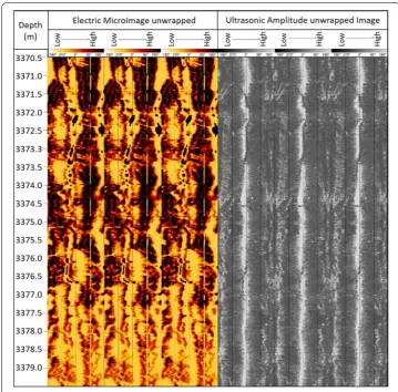
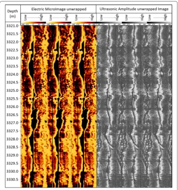
Qualitative analysis of recorded images reveals a feature-rich borehole with clear evi-dence of vertical drilling-induced features and petals in both static and dynamic nor-malization window especially on ultrasonic amplitude images (Fig. 2) (Menger 1994; Deltombe and Schepers 2001; Holl and Barton 2015). The borehole breakouts manifest themselves largely in images with a clear 180° opposite directions (Fig. 2). Tensile frac-tures and other drilling-induced fracfrac-tures manifest themselves at about 90° azimuth with respect to observable large breakouts forming rib-like structures which may emerge in larger petals—centerline features visible especially on the ultrasonic image towards the bottom of exemplified image, see Figs. 2 and 3 (Davatzes and Hickman 2005; Tingay et al. 2008; Rajabi et al. 2016). A closer look into lateral extension of the breakout mani-festation in electrical microimage compared with ultrasonic image shows that the aper-ture extracted from the electrical microimage is three orders larger than the aperaper-ture observed on ultrasonic images. Furthermore, we chose an exemplification interval where the eccentralization of ultrasonic images is not very prominent and display the images side by side (3 times 360°) to eliminate visual obstruction at azimuths 0° and 360°. Images are displayed in Fig. 4 and reveal aggressive hole damages with petal features which can be observed along the well especially in ultrasonic images. These observations, corrobo-rated with core sample analyses (Zierenberg et al. 2017) and inverse multigeophysical inversion (Hokstad and Tanavasuu-Milkeviciene 2017), lead to hypothesizing a mecha-nism of fracturing which is driven by temperature, low pressure and intersections with vertical sheeted dyke structure. The scope of the current article is to investigate further the initial fracture mechanism based on thermomechanical stress mechanism.
Fig. 2 Example of electrical microimage and ultrasonic image from RN‑15/IDDP‑2 wells with associated preliminary feature extractions (courtesy of Equinor and HS Orka). Observe large variation on azimuthal breakouts picking given by angular extension of the feature on the given images. Vertical white stripe on the ultrasonic image is an artifact from tool eccentralization, which adds to complexity of analysis
Numerical simulations
Observation‑driven modeling
Based on data and observations, the following main assumptions are held:
• The rock matrix has brittle elasto-plastic material properties.
• The porosity of the matrix is below 3%. As a consequence, it is considered reasonable to neglect the poroelastic effects (referring to the poroelasticity theory, this would mean assuming a zero Biot coefficient, which can be supported in such a situation, see Fjar et al. (2008), sections 1.3, 2.9 and 6.2; subsequently effective stresses are sim-plified and assumed as total stresses).
• The hole stability is ensured mainly by the rock matrix rigidity, with little influence from fluid pressure in the fractures of the surrounding rock.
• The rock has a fine-grained texture, with heterogeneous grain size and different min-eral grain composition.
The stress state has a strong influence on the failure initiation and propagation, but we lack quantitative data to make solid assumptions. Hence, it was decided to work with a series of possible scenarios for the stress state (see "Numerical approach" section).
Logging images reveal numerous features, between other breakouts and induced fractures. From the drilling operation without any return of fluid to surface (for depths beyond around 3300 m) we can assume that the pressure in the wellbore during drilling was very close to the pressure in the fluid-filled fracture systems intersected by the well. With this limited hydraulic pressure in the well, it is not expected to observe drilling-induced fractures in conventional wells. A possible explanation for this observation is cooling-induced fracture (e.g., Yan et al. 2014). In such high-temperature environments, cooling of the rock necessarily occurs during drilling operations (even before dedicated thermal stimulation). In the following, we provide insight into the initial fracture mecha-nism based on thermomechanical stress mechamecha-nism.
The role of the thermal stimulation is often unclear, and determining which mecha-nisms lead to observed injectivity increase is still challenging (Flores et al. 2005; Grant et al. 2013; Héðinsdóttir 2014). Covell (2016) shows that thermal stimulation is driven by thermal contraction caused by the significant temperature difference between cold injection fluid and hot reservoir rock. The involved mechanisms lead to opening pre-existing discontinuities (contraction of discontinuity walls) or creating new ones. The thermal solicitation induces differential strains at the origin of thermo-mechanical stresses. When these stresses exceed the mechanical resistance of the rock, micro-cracks and failures could appear. Strains at the origin of this process can be mainly due to two causes: on the one hand, a thermal gradient in the rock mass, on the other hand, the heterogeneity of the grain contraction in the rock matrix. Because of this heterogeneity, two adjacent minerals can contract at different rates and this can gen-erate uneven strains at the grain boundary (Wanne and Young 2008). In addition, pet-rographic characteristics (including grain size, grain shape, packing density, packing proximity, degree of interlocking, type of contacts and mineralogical composition) are known to affect mechanical properties (Ulusay et al. 1994). A critical review con-cerning DEM and its application to borehole stability was proposed by Kang et al. (2009). Santarelli et al. (1992) were among the first to study borehole stability using DEM. Yamamoto et al. (2002) used DEM to study the wellbore instability of lami-nated and fissured rocks. Karatela et al. (2016) studied the effect of in situ stress ratio and discontinuity orientation on borehole stability in heavily fractured rocks using DEM. DEM seems fairly adapted to take into account the physical phenomena at the granular phase level (micro scale), and to analyze their impact on the mechani-cal behavior of the near-wellbore zone (macro smechani-cale). We propose to implement this approach using the code Particle Flow Code—2 Dimensions (PFC2D) (Itasca Consult-ing Group Inc. 2008a, b), and to question the role of thermal loadConsult-ings in the wellbore. Chemical interaction of the drilling fluid may play a role in the thermal stimulation, for instance, through dissolution or precipitation of the minerals, triggered by tem-perature change. The quantification of these chemical effects in the specific context of IDDP-2 remains a scientific challenge. Thus, in the absence of available data, indirect chemical effects of thermal stimulation are not considered in this study.
It is worth mentioning that the thermal stimulation by injecting cold water may not necessarily have a long-term effect because of the thermal expansion and closure of fractures during production. Only the naturally propped fractures keep some perme-ability and hence improve productivity.
Numerical approach
PFC2D calculates the movement and interaction of stressed assemblies of rigid circu-lar particles using the DEM. As a discrete element code, it allows finite displacements and rotations of discrete bodies (including complete detachment), and recognizes new contacts automatically as the calculation progresses. The setup is composed of distinct particles that displace independently of one another, and interact only at contacts or interfaces between them. The calculations performed in the DEM alternate between the application of Newton’s second law to the particles and a force–displacement law at the contacts, characterized by normal and tangential stiffnesses. Newton’s second law is used to determine the motion of each particle arising from the contact and body forces acting upon it, while the force–displacement law is used to update the contact forces arising from the relative motion at each contact (Itasca Consulting Group Inc. 2008a).
For a plutonic rock, we choose bonding behavior for contacts (also called “parallel bond”—PB), which allows to reproduce the behavior of cohesive materials (Potyondy and Cundall 2004; Itasca Consulting Group Inc. 2008b). A rupture criterion based on the beam theory is used for PB; when the bond stress exceeds its yielding strength (in tension or in shear), the bond breaks.
The thermal option of PFC2D allows simulation of transient heat conduction and stor-age in particles and development of thermally induced displacements and forces. Each particle can be seen as a heat reservoir. The temperature (Ti, °C), the specific heat coef-ficient (Cv, J kg−1 °C−1) and the linear thermal expansion coefficient (α, °C−1) are ini-tialized for each particle. The thermal power can be transmitted between two particles via a thermal pipe (contact between two particles). The parameters related to a thermal pipe are pipe length (Lp, m) and thermal resistance (Rth, °C W−1 m−1). When particles (i and j) at different temperatures (Ti and Tj) are connected by a thermal pipe, a heat flux (Qp, W) takes place in the thermal pipe (Itasca Consulting Group Inc. 2008b):
The temperature increment (ΔT, °C) of the reservoir can be obtained by
where m (kg) is the mass of the reservoir and Δtth (s) is the thermal time step. Note that by convention an increase of temperature is associated with a positive thermal power. Finally, the radius of the particle (R m) is changed as a consequence. We compute the radius increment (ΔR m) through
The integration of radii increment in the force–displacement law creates induced mechanical response of the system.
(1)
Qp= Ti −Tj
RthLp
.
(2)
T = Qp
mCv tth,
(3)
Numerical settings and scenarios
The calculation setup consists of a two-dimensional cross section perpendicular to the well. The numerical simulations focus on the deepest part of the well. As far as possible, the conditions observed at 4560 m MD of IDDP-2 are used in the numerical simulations. The wellbore section is assumed to be 21.6 cm (8.5 in.). The temperature of the rock is assumed to be 426 °C (corresponding to the fluid temperature measured at the end of drilling). For thermal stimulation, we assume a temperature of 30 °C for the injected fluid (corresponding to the targeted temperature of the cooling fluid). Please note that temperatures recorded during logging operations are above 70 °C, thus using 30 °C
Table 1 Description of the four configurations considered to address uncertainties on the stress state
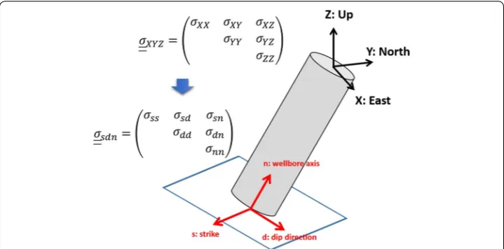
The stress magnitudes are given in 3D in the vertical/horizontal system (here assumed to be the principal stress state) and their components in the 2D plane perpendicular to the wellbore axis (obtained by a linear transform, see Fig. 5). σ1: major
principal stress, σ2: intermediate principal stress. σv: vertical stress, σH: maximum horizontal stress, σh: minimum horizontal stress, σdd: stress component in dip direction of the 2D plan, σss: stress component in strike direction of the 2D plan, τsd: tangential shear stress component in the plane perpendicular to the well
Name “Andersonian” stress state (MPa) Transformed stress
state, aligned with a local coordinate system which is aligned with the wellbore axis (MPa)
Tectonics σv σH σh σss σdd τsd
Case A Intermediary normal/strike‑slip fault (σv = σH= σ1) 134 134 60 125 85 21 Case B Normal fault—“low” horizontal isotropic stress (σv=σ1) 134 60 60 60 79 0 Case C Strike‑slip fault (σH=σ1 and σv=σ2) 134 180 60 166 89 33 Case D Normal fault—“high” horizontal isotropic stress (σv=σ1) 134 80 80 80 94 0
Fig. 5 Sketch of the stress state rotation. The transformed stress is obtained through (i) rotation of principal stresses from 30° along the vertical axis to be in the global coordinate system (Y south–north, X west–east,
Z up–down); (ii) rotation of 40° along the vertical axis to align with the dip direction of the wellbore (Y2
overestimates the cooling during drilling operations (but may be appropriate for the subsequent thermal stimulation). The direction of the wellbore dip direction is N220°E and the deviation from the vertical is approximated at 30°. The modeled 2D cross section is thus oriented N130°E–60°NE.
We focus our study on the behavior of the matrix of the fine-grained-textured rock. The well-detailed description of the dolerite (weekly report IDDP-2, 2016) cored at 4 km depth is used as a reference for the numerical rock model. Deeper coring shows that similar rocks exist in the deeper part of the wellbore.
The four scenarios proposed to scan the range of possible stress states are described in Table 1 for classical coordinate system defined by Andersonian faulting theory, and the corresponding stress state in the 2D cross section normal to the wellbore axis (Fig. 5). In all cases, we consider the vertical direction as the principal stress axis, and we estimate its magnitude at 134 MPa at 4560 m MD depth. The expected horizontal stress magni-tudes are within the range of data extrapolated from Batir et al. (2012), i.e., between 60 and 180 MPa.
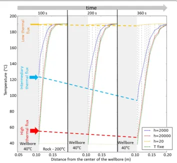
The impact of the thermal flux at the wellbore boundary and of the fluid pressure in the wellbore are evaluated through a parametric study. Investigated fluid pressures in the wellbore are from 34 MPa (measured pressure in the well) to 104 MPa. The heat flux is a linear function of the temperature differential between the rock and the fluid in the well-bore and of the heat transfer coefficient. This coefficient is a quantity that empirically translates the heat exchanges between the circulating fluid and the solid. For the sake of clarification, Fig. 6 illustrates the impact of the choice of heat transfer coefficients on temperature fields. With low values, the heat transfer is slower and the particles of the wellbore need more time to reach the target temperature (Fig. 6). The heat transfer coef-ficient depends notably on the fluid velocity in the wellbore and on the fluid properties. Due to insufficient data, we chose two extreme values for the heat transfer coefficient:
• a low value (1000 W m−2 K−1) simulating a slow cooling of the rock mass on the
boundary of the wellbore;
• a very high value (10,000 W m−2 K−1) simulating an instantaneous cooling of the
rock mass on the boundary of the wellbore.
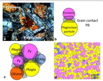
Fig. 7 Elaboration of the numerical rock model: conceptualization and geometric setup. a Thin section of the dolerite from RN‑15/IDDP‑2 (courtesy of HS Orka). b Conceptualisation: each crystal grain is modeled by a numerical particle; contacts between grains are modeled by parallel bonds (PB). c Schematic view of a detail of the numerical rock model: bonded particles aggregate (Py pyroxene, Plagio plagioclases, TiMg
Numerical rock setup
The elaboration of the numerical rock model setup is a preliminary essential task, often difficult due to insufficient data and thus high level of uncertainties. Before any numerical modeling, the real rock (here a dolerite) is conceptualized according to the role of each mineral phases in the behavior of the rock (more details in Peter-Borie et al. 2011, 2015). The dolerites are typical shallow intrusive bodies; they are micro-grained, composed entirely of 1–5-mm-wide crystallized minerals without glassy matter. Grains or crystals are interlocked as the growth of each crystal has stopped on other crystals (MacKenzie and Adams 1999). For the numerical dolerite model, each numerical particle represents a mineral grain or crystal (Fig. 7). Parallel bonds (PB) model the contacts between grains (Fig. 7). Note that in grained rock, failure can occur between the grains as well as inside a grain (following then the weakest paths like twins leading to cleavage plans—Kranz 1983). In the numerical rock model, fail-ure can occur only between particles. To fit with the reality, mechanical properties of the PB are the mean properties of the surrounded particles, a failure between two particles can then be interpreted as an intergrain or intragrain failure.
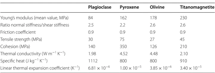
Following the conceptualization step, the properties of the numerical particles and bond are assigned. In this regard, quantified data from studied or analogue rock are required. For the present application case, the coring of fine-grained dolerite retrieved at 4090.6 m depth (Zierenberg et al. 2017) provided detailed information on the rock composition (pyroxene 40%, plagioclase 55%, titanomagnetite 5%, grain size around 3 mm). The particles of the numerical dolerite model follow the same distri-bution. The heterogeneity of particles size is represented through the implementation of a particle-size distribution centered on 3 mm.
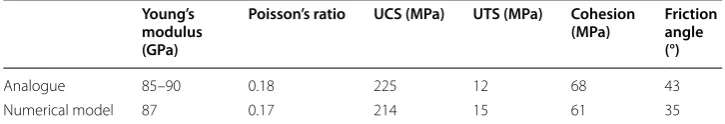
At the time of the study, macroscopic mechanical and thermal data were not available from the IDDP-2 cored samples. Thus, we chose a limited analogue rock with available macroscopic properties. Since petrographic characteristics affect mechanical proper-ties, analogues are selected depending on the proximity in terms of rock petrographic characteristics as mineral composition and grain size. A North African gabbro, charac-terized by Keshavarz (2009), is retained as reference analogue. It contains almost 40% pyroxene and 60% plagioclase, with traces of other elements (among others magnetite). Laboratory tests performed on pressurized (stepwise up to 650 MPa) and heated (step-wise up to 600 °C) samples provide mechanical properties of the analogue rock covering
Table 2 Mechanical, thermal and thermo-mechanical properties of particles
after calibration
Plagioclase Pyroxene Olivine Titanomagnetite
Young’s modulus (mean value, MPa) 84 162 178 230
Ratio normal stiffness/shear stiffness 2.5 2.2 2.6 2.6
Friction coefficient 0.9 0.9 0.9 0.9
Tensile strength (MPa) 30 75 27 45
Cohesion (MPa) 140 350 126 210
conditions similar to those expected in the bottom of IDDP-2. As micro-gabbro/doler-ite have very low porosity [below 0.5% in the analogue rock (Keshavarz 2009), matrix porosity between 3.6 and 0.1% (no microporosity included) for the cored dolerite (Clau-dia Kruber, Equinor internal report in progress)], we assume that the pores can be seen as singularities in the rock matrix. The numerical rock model does not integrate the rock porosity. Therefore, in our numerical approach, no poroelastic effects are considered. The heat transfer process is thus limited to conduction between grains.
The range of values of the mechanical, thermal and thermo-mechanical micro-prop-erties (at the particle scale) has been first delimited according to a literature review on the properties of minerals (Simmons 1965; Carmichael 1989; Guéguen and Palciauskas 1992; Clauser and Huenges 1995). The properties must be physically consistent with the mineral phase characteristics and have to enable the reproduction of the macroscopic mechanical and thermo-mechanical behavior of the rock. The definitive calibration of the numerical particles and bonds particles is performed by fitting results of mechani-cal and thermal numerimechani-cal tests (Uniaxial Compressive Strength—UCS, Ultimate Tensile
Table 3 Mechanical properties of the selected analogue rocks and of the numerical rock model
UCS: uniaxial compressive strength, UTS: ultimate tensile strength
Young’s modulus (GPa)
Poisson’s ratio UCS (MPa) UTS (MPa) Cohesion
(MPa) Friction angle (°)
Analogue 85–90 0.18 225 12 68 43
Numerical model 87 0.17 214 15 61 35
Strength—UTS, Triaxial and Thermal conductivity tests) with the macroscopic proper-ties of the analogue rock (see final values of micro-properproper-ties in Table 2, and resulted macro-properties computed from numerical tests in Table 3).
Near‑wellbore setup
The calculation setup concerns a 2D plane perpendicular to the wellbore axis at 4560 m MD depth. The definition of the near-wellbore setup needs to take into account an adequate extended area around the wellbore—at least three times the diameter of the wellbore (here 21.6 cm–8.5 in.) to limit the impact of boundary con-ditions on the numerical results. A significant number of particles are needed to build up such a large setup while keeping the size distribution close to the mineral size level (here close to an average of 3 mm). To push away the boundary conditions, the DEM near-wellbore model is embedded within a continuum-mechanics-based frame describing the region far away from the wellbore (FLAC Itasca Consulting Group Inc. 2002). The PFC2D simulation setup size is 1.05 m × 1.05 m, integrating more than 141,500 particles, and is embedded within a 5.25-m × 5.25-m FLAC mesh (Fig. 8). The coupling method between the continuum model and the discontinuous model is realized by an edge-to-edge approach for which the relevant overlapped elements are, respectively, segments of mesh in FLAC and a series of particles in PFC2D (Xiao and Belytschko 2004). A detailed description of the near-wellbore setup and of the PFC2D/FLAC coupled calculations is available in Shiu et al. (2011).
Simulation stepwise
The numerical simulation is performed stepwise with the aim to reproduce, as far as possible, the state of the rock in the vicinity of the wellbore before the thermal stimu-lation. Randomization is used for the construction of the numerical model. The radius of each particle is randomly drawn following the normal distribution N(1.37, 0.62) for pyroxene and plagioclase, and following N(1.25, 0.5) for titanomagnetite (based on cores observations). A periodic sample duplication process is used to build the numerical model faster.
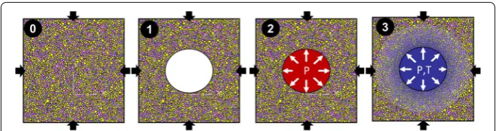
Once the numerical setup is constructed and confined under a small confining pres-sure (which is always less than its corresponding in situ stress), it is loaded with its in situ stress which is presented in Fig. 9, step 0. We use the full-strain method (Itasca Consulting Group Inc. 2008c) for which a displacement increment is applied to each particle. Cycles are performed between two increments of displacement to reach a new mechanical equilibrium. Note that no contact breakage is allowed during the stress installation cycling. Thus, a pure elastic deformation is performed in this step. This method is very efficient when a large number of particles are included in the numerical model.
After the initial stress field is established, the borehole drilling is simulated by remov-ing the particles located on the wellbore surface (Fig. 9 step 1). To avoid a sudden increase of the unbalanced forces of particles placed on the surface of the wellbore, lead-ing to numerical instabilities, a force-reduction procedure is used at this step to release progressively the unbalanced forces of particles situated along the wellbore surface (Shiu et al. 2011). Note that this step is a very rough and simplified approximation of the drill-ing impact on the formation stability. On the one hand, the impact of the drilldrill-ing bit at the excavation step is not considered. On the other hand, the pressure considered in the wellbore is assumed zero, due to limitation in the calculation procedure, which can lead to damage overestimation as pressure actually exists in the well during real drilling at ECDs (equivalent circulation densities) even above the static fluid column.
During the fluid injection step of the calculation schedule, the wellbore is subjected to a hydraulic pressure and to a thermal loading. The fluid injection is assumed to act only on particles forming the wellbore surface. A specific procedure (Itasca Consulting Group Inc. 2008c; Shiu et al. 2011) is used to detect a set of closed linked particles (con-nected by parallel bonds) around the wellbore. These particles are recorded in a specific list and will be referred to as the wellbore list in the following description. To simplify the numerical modeling setup, and to limit the computational time, the hydraulic pres-sure and the thermal loading are applied in two steps. The hydraulic prespres-sure is applied first (Fig. 9 step 2) and the thermal loading (Fig. 9 step 3) takes place later (assuming that no significant thermal propagation occurs before the hydraulic pressure is fully installed on the wellbore surface). The underlying assumption is that the characteristic time for pressure effects is far shorter than the characteristic time for thermal effects. The list of the wellbore particles is updated automatically when cracks appear between particles in the wellbore list. Hence, once the cracks start propagating from the wellbore, the injec-tion pressure and the fluid temperature can penetrate into the crack as well.
Results
Simulation of the drilling of the well
Fig. 10 Results of simulations, after drilling, for the four stress states (see "Numerical approach" section for definition of cases A, B, C and D). Each red point corresponds to the apparition of a tensile crack, each blue point corresponds to the occurrence of a shearing crack. The total number of cracks is mentioned in each subplot. The field of view for each subplot is 1 m × 1 m
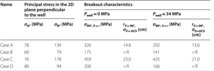
Table 4 Results of the analytical approach for breakouts
The computation of the borehole potential damage is linked to no to low wellbore fluid pressure (Pwell). σ90°, R =r is the circumferential stress at the wellbore boundary in the direction of the minimal 2D stress, rθ =90°, σθ = UCS is the distance
from the wellbore center where the circumferential stress is equal to the UCS of the dolerite (214 MPa), in the direction of the minimal 2D stress, R is the radius of the borehole. Principal stresses in the cross section perpendicular to the well are obtained by diagonalization of the stress state (σss, σdd, τsd) mentioned in Table 1 and are thus slightly different from horizontal principal stresses
Name Principal stress in the 2D plane perpendicular to the well
Breakout characteristics
Pwell= 0 MPa Pwell= 34 MPa
σA* (MPa) σB* (MPa) σ90°, R = r (MPa) rθ = 90°, σθ = UCS (cm)
σ90°, R = r (MPa) rθ = 90°, σθ=UCS
(cm)
Case A 76 134 326 14.8 292 13.6
Case B 60 79 175 < R 141 < R
Case C 76 178 459 23.0 425 21.0
of cracks is four times less than for case C. It leads locally to a rock caving up to 1 cm. Other stress states (B and D) lead to a limited number of cracks.
These numerical results are compared with results obtained with the analytical Kirsch equations (see Appendix), presented in Table 4. The analytical solution pre-dicts that breakout will occur for cases A and C for both zero fluid pressure and in case it is equal to 34 MPa.
There is good agreement between the analytical and numerical results. Most cracks in numerical results are in the area stress from analytical solution exceeds the rupture cri-terion. The ratios of cracks in this area compared to all cracks are, respectively, 88% and 89% for cases A and C for zero fluid pressure in the wellbore. Some differences between analytical and numerical results can nevertheless be noted (Fig. 11):
• In numerical simulation, cracks coalesce until creating a caved area; this area rep-resents only a limited part of the area where the rupture criterion is exceeded in the analytical model.
• Cracks in the numerical model also occur outside of the area where the rupture
criterion is exceeded according to the analytical solution.
Several possible explanations can be suggested to discuss these differences:
• As contact properties depend on the adjacent particle properties, the PB do not
have all the same strength (the criterion of the analytical solution is the mean strength of the rock). Cracks may occur outside of the analytical breakout area when the strength of the PB is locally exceeded by the stress, even if it is lower than the criterion. Conversely, stronger bonds may resist in the numerical model, even if the analytical area predicts rupture.
Fig. 12 Confrontation of the numerical results and of the logging images. a Numerical results were transformed to logging‑like images. The color intensity corresponds to the distance between the boundary of the wellbore and the center of the wellbore, after drilling, for case C, with zero fluid pressure in the wellbore. θn is the angle measured from the direction of maximum stress. b Electrical microimage (extracted from the image presented in Fig. 2). The azimuthal origin for numerical results was adjusted manually for qualitative comparison (θl and θn scales have not the same origin)
• Because of the heterogeneity of the properties of the particles and of the PB, stress local modification can occur. Thus, locally, a higher stress can lead to PB breaking, or a lower stress to PB integrity.
• The caving in the breakout area will affect the stress further—this case cannot be
taken into account in the analytical solution.
The qualitative analysis of the in situ logging images of the RN-15/IDDP-2 reveals numerous features that may be interpreted as breakout. The results of the numerical simulation of the effect of the drilling in the strike-slip regime (case C) could potentially fit these observations (Fig. 12). High resistivity on logging images (black color) might correspond to cavings filled with fluid, thus matching with increased well radius in numerical results. To go beyond, it would be interesting to have better knowledge of the stress state and to have quantitative estimation of breakout caving (with calipers), thus enabling the comparison of caving dimensions (depth and lateral extension).
Impact of increased well pressure
In this section, we discuss the mechanical impact of increased well pressure, without thermal loading effects, with tensile failure as expected result.
Table 5 Results of the analytical approach for the computation of the breakdown pressure (Pfrac)
Following Eq. 14 in Appendix with T=0 and UTS = 15 MPa. Principal stresses in the cross section perpendicular to the wellbore axis are obtained by diagonalization of the stress state (σss, σdd, τsd) mentioned in Table 1 and are thus slightly different from horizontal principal stresses
Name Tectonics Principal stresses Pfrac, UTS=15 MPa
σA* (MPa) σB* (MPa)
Case A Intermediary normal/strike‑slip fault (σv=σH=σ1) 76 134 110 Case B Normal fault—“low” horizontal isotropic stress (σv=σ1) 60 79 116 Case C Strike‑slip fault (σH=σ1 and σv=σ2) 76 178 65 Case D Normal fault—“high” horizontal isotropic stress (σv=σ1) 80 94 161
The numerical work focuses on case C (strike-slip regime). In the simulation, the pressure is applied by 1-MPa increment up to 90 MPa on the wellbore bound-ary. Figure 13 shows the result. The tensile fracture initiates for a well pressure close to 65 MPa, with 3 cm length into the rock matrix. Further stepwise increase of the pressure leads to progressive fracture depth. A pressure in the wellbore higher than 89 MPa is necessary for a wide propagation of the fracture.
For the sake of comparison, results obtained with the Kirsch equations (see Appen-dix) are presented in Table 5. The tensile failure appears for a pressure in the wellbore of 65 MPa, thus in good agreement with the numerical results. For the other stress states, a pressure in the well above 100 MPa is necessary to induce tensile failure.
In the RN-15/IDDP-2 wellbore, the pressure remained limited (below breakdown pressures computed in this section). Neither the analytical solution nor the numeri-cal simulation results can explain the tensile fractures observed by the low well pres-sures. However, numerous features that may be interpreted as tensile fractures are observed in the image logs (see "Logging images" section and Fig. 2). Therefore, we study the effects due to the thermal cooling in the next section.
Cooling effects on wellbore stability
The additional temperature term contributing to the hoop stresses in the analytical solution (Eq. 14 in Appendix) leads to tensile failure in all cases for a cooling larger than 190 °C (Fig. 14) without any need of fluid pressure in the well (Pwell= 0 MPa). In RN-15/IDDP-2 well, the host rock temperature is estimated to be between 426 and 549 °C (see "Geological knowledge" section), which means that any downhole drill-ing fluid temperature below 236 °C is likely to induce tensile fractures. This is in good agreement with the numerous tensile fractures observed on image logs (see "Logging images" section and Fig. 2).
Numerical simulations are proposed here for an in-depth view of the failure under thermal loading. Our motivation is twofold: first, the DEM approach allows to take into account thermal effects at the microscale (notably the differential expansion of the grains of the rock) and thus the approach is indeed more detailed for simulating the thermal
effects. Second, the shape and size of damages can be retrieved and analyzed in compar-ison with observations. We investigate the impact of the thermal flux (through the heat transfer coefficient values) and of the pressure in the well. For the sake of comparison, and after a brief presentation of the stress state impact, a sensitivity analysis is presented.
Thermo‑mechanical tensile failures depending on the stress state
Figure 15 shows the development of the cracks and of the induced fractures by the cracks’ coalescence for the different stress states, in the absence of hydraulic pressure in the wellbore. Tensile fractures developed in all the four cases, as predicted by the analyt-ical results. However, depending on the stress state, the shape, the propagation direction and the intensity of the damage differ. With the largest 2D deviatoric stresses (cases A and C), the fracture propagates in the direction of the 2D maximum stress σB* (perpen-dicular to the direction of breakout caused by drilling, if any). In the most isotropic cases (cases B and D), fractures develop around the wellbore without preferential direction, following the path of least resistance defined by the local mineral distribution.
Impact of the thermal flux at the wellbore boundary
Figure 16 allows the comparison of the development of cracks in the rock depending on the thermal flux through extreme values of heat transfer coefficient for the stress state case C (strike-slip tectonic regime). With a low flux (low heat transfer coefficient value), the kinetics of the fracture development is drastically reduced. The second observation is less intuitive: besides kinetics, the cooling rate influences the shape of fractures. A fast cooling of the rock (high heat transfer coefficient, high thermal
gradient from the beginning of the cooling) creates several tortuous fractures, with dichotomy, while a slow cooling of the rock (low heat transfer coefficient value, pro-gressive increase of the thermal gradient in the rock) allows the focusing of the crack within a single fracture.
Moreover, it should be noticed that the coalescence of cracks observed in the case of high thermal flux can lead to separation of larger pieces of rock as shown in Fig. 17. This may be interpreted as caving on the wellbore images. In this case, cavings are not the result of overly low ECD but are due to the thermal loading. These temperature-induced cavings tend to be oriented in the maximum principal stress direction, contrary to breakouts caused by overly low ECD. The layout of crack development and coales-cence in the case of fast cooling may provide explanations on some logging features: one can observe that the logging image is not symmetric but has a tendency to develop larger on one azimuth than the systematic one (note that the logging image is on a shallower depth than result of numerical modelling).
Impact of the pressure in the wellbore
The hydraulic pressure has a significant influence on the damage in the near-wellbore area as illustrated in Fig. 18. With high well pressure, towards the range of the least com-pressive hoop stress, the induced fractures localize towards a distinct plane with prefer-ential orientation. For a pressure lower than the theoretical breakdown pressure in the wellbore (65 MPa, see "Impact of increased well pressure""section), the induced fracture is more restrained, split and discontinuous. Features observed on the logging images
correspond rather to discontinuous fractures than to very localized fractures. Since pressure in the wellbore was limited, this lends credibility to the model.
Discussion
The presented study may shed light on the effects of the wellbore drilling and of the thermal stimulation in a deep and very hot fine-grained rock. Drilling and pressuriza-tion impacts on the wellbore stability have been studied first. The formapressuriza-tion of break-outs and induced tensile fracture have been successfully described by the calculation results, even though we consider total deconfinement of the wellbore during drilling and no dynamic processes as tools impact in a first approach. Slight differences can be explained by the level of greater detail included in the numerical approach compared to the analytical solution: grain heterogeneity in the rock matrix, caving processes allowed and not pre-defined. From both analytical solution and numerical results, a fluid pres-sure no less than 65 MPa is needed for inducing tensile fracture without considering thermal effects. During the drilling phase and after, the pressure in the bottom of the well is under the breakdown pressure. However, numerous induced fractures have been observed in the logging images; a thermal component appears to be necessary to explain the observations.
In the RN-15/IDDP-2 well, there is a drastic difference in temperature between the fluid in the well and formation, probably higher than 150 °C during the drilling phase and even higher during the thermal stimulation (up to 400 °C). From both analytical and DEM calculations, which take into account thermo-mechanical loadings, this constant thermal stimulation induces tensile fracture. Note that considering the high temperature difference, fluid pressure in the well is not necessary for fracture inducing.
Complementary to the analytical solution, DEM allows a more detailed study of the thermo-mechanical processes; beyond the “macro” thermo-mechanical processes, the impact of the differential behavior of the minerals composing the rock can be considered thanks to a modeling at the grain scale. In addition, this approach allows notably the quantification of the damage around the wellbore, the visualization of the pathway of the induced fractures.
Beyond the above-presented results fitting with the observations, and as for any model, it is important to keep in mind the limitations when analyzing modeling results. Among the model limitations, we can quote the two dimensionality, the matrix consid-ered as impermeable, and the impossibility to generate intragranular cracks.
of the thermal stimulation (depending notably on the flow rate, the temperature at sur-face, the pressure and the composition of the injected fluid). In addition to these influent uncertainties, the influence of the rock model should also be further investigated.
A second layer of uncertainties is introduced when comparing the modeling results with logging images, since these latter are also subject to uncertainties. Besides, note that the logging is performed more than 48 h after drilling while exposing the well to both thermocycling and pressure cycling; as a consequence, comparisons are mainly qualitative, but provide nonetheless a preliminary evaluation on the ability of the numer-ical approach to replicate successfully the observations.
Further investigations and numerical developments are needed to confirm the assumption and for a better understanding of the linked processes. Indeed, some lim-itations of the used version of the numerical code can lead to a misevaluation of the pathway and the propagation speed of the fractures: the energy of propagation of the fractures is not taken into account (Kanninen and Popelar 1985); the stability/instability of fracture growth in and out the zone of increased stress should be further investigated depending on the stimulation mechanism (either thermal or pressure effects). We have observed that the results are not accurately capturing the propagation of fractures into the far field once the close wellbore region is fractured when well pressures are larger than the minimum horizontal stress. The reason for that is found to be in the definition of the 2D plane strain cross section and the definition of the boundary conditions. The principal stress direction of the far field stresses is not aligned with the plane in which the 2D calculations are performed and also the axial stresses are not taken into the lower dimensional setup. For that reason, the system does not recognize that the out-of-plane, far-field stress is not a principal stress direction, but rather rotating with distance from the wellbore. This simplification overestimates the overall resistance against fracturing in the far field which in reality would be simply the minimum horizontal stress and rock resistance. Therefore, a fully 3D setup including all components of the stress tensor is proposed in future studies, which will shed light on stable vs unstable fracture growth beyond the close-wellbore region in the case of inclined wells exposed to temperature and pressure loading. This enhanced setup would then also enable a discussion of the paths of fractures propagating from the well into the far field eventually creating so-called “hackles”.
Further developments are also in progress for interpreting the induced fractures in terms of injectivity and later on also for studying productivity gains. The goal of such future simulations will be to enable the numerical reproduction of transient productiv-ity loss as the previously created fracture closes due to thermal expansion of the matrix.
Conclusion
• The long computational time resulting in limited number of possible investigations
in the parametric study;
• The two dimensionality of the model leading to a poor capture of the propagation of fractures into the far field;
Some of these limitations can be improved in future works, in particular, by consid-ering a 3D setup.
Nonetheless, numerical results are consistent with the results of the analytical solutions. According to the numerical results, as well as to the analytical solution, and fitting with the observations in RN-15/IDDP-2, breakouts result from the drill-ing process—argudrill-ing for a quite high local deviatoric stress—and tensile fractures appear because of the high thermal loading. Overpressure in the wellbore speeds up the process.
Moreover, the numerical simulation allows a deeper investigation into the effect of the drilling and into the thermal stimulation. In particular, the impact of the differen-tial behavior of the minerals composing the rock can be considered thanks to a mod-eling at the grain scale. In addition, this approach notably allows the quantification of the damage around the wellbore and highlights the caved areas and the pathway of the induced fractures in the near field.
As emphasized, a fresh aspect of this study is the consideration of the thermal flux at the wellbore boundary. We have shown that a high thermal flux between the fluid in the wellbore and the rock leads to tortuous pathways for induced fractures; In this case, pieces of rock can be separated from the rock mass. This could be one explana-tion for the observed induced fractures and cavings in the logging images, oriented perpendicular to the direction of breakouts due to low ECD.
Abbreviations
DEM: discrete element method; ECD: equivalent circulation density; EGS: enhanced/ engineered geothermal system; IDDP: Iceland Deep Drilling Project; MD: measured depth; PB: parallel bond; PFC2D: particle flow code—2 dimensions; UCS: uniaxial compressive strength; UTS: ultimate tensile strength; VD: vertical depth.
List of symbols
perpendicular to the well (MPa); τrθ : tangential shear stress around the borehole (MPa);
Cv: specific heat coefficient (J kg−1 °C−1); E: Young’s modulus (GPa); Lp: pipe length (m);
m: mass of the heat reservoir (kg); Pfrac: fracture pressure (MPa); Pwell: well pressure (MPa); Pp: pore pressure of the formation (MPa); Qp: power in the thermal pipe (W);
r: distance from the center of the hole (m); R: radius of the borehole (m); Rth: thermal resistance (°C W−1 m−1); T
i: temperature of the numerical particle i (°C); Tj: temperature of the numerical particle j (°C).
Authors’ contributions
BRGM’s authors performed modeling work and prepared the core of the manuscript. Equinor’s authors provided data from wellbore logging and enriched the discussion part. HsOrka provided data from RN‑15/IDDP‑2. All authors read and approved the final manuscript.
Author details
1 BRGM, 3 av. C. Guillemin, BP36009, 45060 Orléans Cedex 2, France. 2 Equinor ASA, Research and Technology, Rotvoll, Norway. 3 HsOrka, Svartsengi, 240 Grindavík, Iceland.
Acknowledgements
We would like to thank Kati Tänavsuu‑Milkeviciene (Equinor) and Claudia Kruber (Equinor) who helped with the geology, mineralogy and porosity analyses; Théophile Guillon (BRGM) and Arnold Blaisonneau (BRGM) for fruitful discussion on modeling issues. The authors are grateful to the editor and to the two anonymous reviewers for their helpful comments and advice.
Competing interests
The authors declare that they have no competing interests.
Availability of data and materials Not applicable (commercial code).
Funding
This study was part of the DEEPEGS project, which received funding from the European Union HORIZON 2020 research and innovation program under Grant agreement no. 690771.
Appendix: Simplified analytical approach for computation of stress development in the near-wellbore area
We propose to compute the analytical solution for the stress development in the near-wellbore area to evaluate the risk of breakout and breakdown. The proposed analytical solution is a simplified one: it requires the assumption of a wellbore parallel to princi-pal stress that is not the case of the deep part IDDP-2 for the four stress states consid-ered. For a cylindrical hole in a thick, homogeneous, isotropic, elastic plate subjected to effective minimum and maximum stresses (absolute values of minimum and maximum stresses are noted σA* and σB* hereafter), disregarding any thermal stresses, the following equations apply (Kirsch 1898 in Zoback et al. 1985):
(4) σr =
1 2
σB∗+σA∗
1− R
2 r2 +1 2
σB∗−σA∗
1−4R
2
r2 +3 R4 r4
cos 2θ +�PR
2
r2,
(5) σθ =
1 2
σB∗+σA∗
1+R
2 r2 −1 2
σB∗−σA∗
1+3R
4
r4
cos 2θ−�PR
2
r2,
(6) τrθ = −
1 2
σB∗+σA∗
1+2R 2
r2 −3
R4 r4
where σr is the radial stress, σθ is the circumferential stress, τrθ is the tangential shear stress, R is the radius of the hole, r is the distance from the center of the hole, θ is the azimuth measured from the direction of σB* and ∆P is the difference between the fluid pressure in the borehole and the pore pressure (positive indicates overpressure in the borehole).
At the well boundary, when r=R, the set of equations becomes
The most critical stresses at the well boundary, called hoop stresses, occur for σθ when
θ equals 0° (minimal stress value, i.e., maximum tensile stress) and when θ equals 90° (maximal stress value, i.e., maximum compressional stress):
According to the analytical model, and for a Mohr–Coulomb strength criterion, dam-ages occur if σ0◦ reaches the UTS or if σ90◦ exceeds the UCS. In the first case,
drilling-induced tensile fractures develop in the direction of the maximum stress; the fluid pressure in the well has reached the so-called breakdown pressure. On the contrary, for θ= 90°, damages appear in the form of breakout in the direction of the minimum stress; high pressure acts as a stabilizer.
Thermal effects can be integrated into the analytical model, by adding the thermal stress coefficient in the equations (Stephens and Voight 1982): αLE�T/(1−ν), where αL is the linear coefficient of thermal expansion, E the Young’s modulus, ΔT the tempera-ture difference between the fluid in the wellbore and the rock (ΔT is negative for cool-ing), and ν the Poisson’s ratio. The equations for σθ at the well boundary become
From these equations, it can be seen that the thermal effects favor the occurrence of induced fractures when cooling the wellbore ( σ0◦ decreases since T is negative for
cooling, thus the failure may occur sooner). In the present case, in the absence of pore pressure, P=Pwell and thus the fracture pressure Pfrac considering the thermal effect is
(7)
σr =�P,
(8) σθ =σB∗+σ
∗
A−2
σ∗
B−σ
∗
A
cos 2θ −�P,
(9) τrθ =0.
(10)
σ0◦ =3σ∗
A−σ
∗
B−�P,
(11)
σ90◦ =3σ∗
B−σ
∗
A−�P.
(12) σ0◦ =3σ∗
A−σ
∗
B−�P+ αE�T (1−ν),
(13) σ90◦ =3σ∗
B−σ
∗
A−�P+ αE�T (1−ν).
(14) Pfrac=3σ∗
A−σ ∗
B+UTS+
αE�T
Publisher’s Note
Springer Nature remains neutral with regard to jurisdictional claims in published maps and institutional affiliations.
Received: 14 April 2018 Accepted: 16 August 2018
References
ALT advanced logic technology, acoustic borehole imagers and specifications ABI43. https ://www.alt.lu/pdf/abi_2013. pdf. Accessed 26 Feb 2018.
Baujard C, Genter A, Dalmais E, et al. Hydrothermal characterization of wells GRT‑1 and GRT‑2 in Rittershoffen, France: implications on the understanding of natural flow systems in the rhine graben. Geothermics. 2017;65:255–68. Batir J, Davatzes N, Asmundsson R (2012) Preliminary model of fracture and stress state in the Hellisheidi geothermal
field, Hengill volcanic system, Iceland. In: Thirty‑Seventh Workshop on Geothermal Reservoir Engineering. Palo Alto: Stanford University; 2012.
Carmichael RS. Practical handbook of physical properties of rocks and minerals. Boca Raton: CRC Press; 1989. Clauser C, Huenges E. Thermal conductivity of rocks and minerals. Rock Phys Phase Relat. 1995;1(3):105–26.
Covell C. Hydraulic well stimulation in low‑temperature geothermal areas for direct use. Thesis of 60 ETCS credits. Master of Science in Energy Engineering, Iceland School of Energy; 2016.
Davatzes N, Hickman S. Comparation of acoustic and electrical image logs from the Coso geothermal filed. In: Thirty‑ Seventh Workshop on Geothermal Reservoir Engineering. Palo Alto: Stanford University; 2005.
Deltombe JL, Schepers R. Combined processing of BHTV travel time and amplitude images. In: Proc. Int. Symp. Borehole geophysics for minerals, geotechnical and groundwater applications. Colorado: Golden; 2001. vol. 7, p. 29–42. EGEC. 2016 EGEC geothermal market report, key findings, 6 edn; 2017.
Fjar E, Holt RM, Raaen AM, et al. Petroleum related rock mechanics, vol. 53, 2nd edn. New York: Elsevier Science; 2008. Flores M, Davies D, Couples G, Palsson B. Stimulation of geothermal wells, can we afford it? In: Proceedings of the World
Geothermal Congress, Antalya, Turkey, 2005.
Foulger GR, Du Z, Julian BR. Icelandic‑type crust. Geophys J Int. 2003;155:567–90.
Friðleifsson GO, Bogason SG, Stoklosa AW, et al. Deployment of deep enhanced geothermal systems for sustainable energy business. In: Proceedings, European Geothermal Congress, Strasbourg; 2016.
Friðleifsson GO, Elders WA. The Iceland Deep Drilling Project geothermal well at Reykjanes successfully reaches its super‑ critical target. Geotherm Resour Counc Bull. 2017a;2017:30–3.
Friðleifsson GO, Elders WA. Successful drilling for supercritical geothermal resources at Reykjanes in SW Iceland. Geo‑ therm Resour Counc Bull. 2017b;41:1095–107.
Friðleifsson GO, Elders WA, Zierenberg RA, et al. The Iceland Deep Drilling Project 4.5 km deep well, IDDP‑2, in the seawater‑recharged Reykjanes geothermal field in SW Iceland has successfully reached its supercritical target. Sci Drill. 2017;23:1–12.
Grant MA, Clearwater J, Quinao J, et al. Thermal stimulation of geothermal wells: a review of field data. In: Proceedings of the thirty‑eighth workshop on geothermal reservoir engineering, Stanford University, Stanford; 2013.
Gudmundsson A. Dynamics of volcanic systems in Iceland: example of tectonism and volcanism at juxtaposed hot spot and Mid‑Ocean Ridge systems. Annu Rev Earth Planet Sci. 2000;28:107–40.
Guéguen Y, Palciauskas V. Introduction à la physique des roches. Hermann edit; 1992.
Héðinsdóttir H. Mechanisms of injectivity enhancement in the thermal stimulation of geothermal wells. Master Thesis, Department of Earth Sciences ETH Zürich Geological Institute Engineering Geology, 2014.
Heidbach O, Tingay M, Barth A, et al. The World Stress Map database release, 2008.
Heidbach O, Rajabi M, Reiter K, Ziegler M. The WSM Team World Stress Map database release. 2016 GFZ data services, 2016.
Hokstad K, Tanavasuu‑Milkeviciene K. Temperature prediction by multigeophysical inversion: application to the IDDP‑2 well at Reykjanes, Iceland. Geotherm Resour Counc. 2017;41:1141–52.
Holl HG, Barton C. Habanero field—structure and state of stress. In: Proceedings World Geothermal Congress 2015, Melbourne; 2015.
Itasca Consulting Group Inc. PFC2D—Particle flow code in 2 dimensions, Version 4.0, Theory and background manual. Minneapolis: Itasca; 2008a.
Itasca Consulting Group Inc. PFC2D/3D (Particle flow code in 2/3 dimensions), Version 4.0, MN: ICG. Minneapolis; 2008b. Itasca Consulting Group Inc. Fast lagrangian analysis of continua, 4th ed., 4.0 Minneapolis: Itasca; 2002.
Itasca Consulting Group Inc. PFC2D—Particle Flow Code in 2 Dimensions, Ver. 4.0, FISH Reference Manual. Minneapolis: Itasca; 2008c.
Kang Y, Yu M, Miska SZ, Takach N. Wellbore stability: a critical review and introduction to DEM. Soc Pet Eng. 2009. https :// doi.org/10.2118/12466 9‑MS.
Kanninen MF, Popelar CH. Advanced fracture mechanics. Oxford: Oxford University Press; 1985.
Karatela E, Taheri A, Xu C, Stevenson G. Study on effect of in situ stress ratio and discontinuities orientation on borehole stability in heavily fractured rocks using Discrete Element Method. J Pet Sci Eng. 2016;139:94–103.
Karson JA. Crustal accretion of thick, mafic crust in iceland: implications for volcanic rifted margins. Can J Earth Sci. 2016;53:1–11.
Keiding M, Lund B. Earthquakes, stress, and strain along an obliquely divergent plate boundary: Reykjanes Peninsula, southwest Iceland. J Geophys Res. 2009;114:1–16.