REVIEW
Benchmark analysis of forecasted
seasonal temperature over different climatic
areas
G Giunta
1, R Salerno
2, A Ceppi
3*, G Ercolani
3and M Mancini
3Abstract
From a long-term perspective, an improvement of seasonal forecasting, which is often exclusively based on climatol-ogy, could provide a new capability for the management of energy resources in a time scale of just a few months. This paper regards a benchmark analysis in relation to long-term temperature forecasts over Italy in the year 2010, compar-ing the eni-kassandra meteo forecast (e-kmf®) model, the Climate Forecast System–National Centers for Environmen-tal Prediction (CFS-NCEP) model, and the climatological reference (based on 25-year data) with observations. Statisti-cal indexes are used to understand the reliability of the prediction of 2-m monthly air temperatures with a perspective of 12 weeks ahead. The results show how the best performance is achieved by the e-kmf® system which improves the reliability for long-term forecasts compared to climatology and the CFS-NCEP model. By using the reliable high-performance forecast system, it is possible to optimize the natural gas portfolio and management operations, thereby obtaining a competitive advantage in the European energy market.
Keywords: Seasonal forecasts, Energy demand, Air temperature predictions, Weather model performance, Benchmark analysis
© 2015 Giunta et al. This article is distributed under the terms of the Creative Commons Attribution 4.0 International License (http://creativecommons.org/licenses/by/4.0/), which permits unrestricted use, distribution, and reproduction in any medium, provided you give appropriate credit to the original author(s) and the source, provide a link to the Creative Commons license, and indicate if changes were made.
Introduction
The advent of computer technology has led scientists to developing complex models to forecast natural gas con-sumption by improving calculation algorithms and using different statistical methods (Smith et al. 1996; Gorucu and Gumrah 2004; Sánchez-Úbeda and Berzosa 2007; Forouzanfar et al. 2010; Soldo 2012). An efficient man-agement of energy distribution system often requires out-look prediction in relation to energy demand (Mirasgedis et al. 2006; Potocnik et al. 2007; Dovrtel and Medved 2011; Oldewurtel et al. 2012; Petersen and Bundgaard 2014), which is strictly related to seasonal weather and climatic trends. Therefore, meteorological information must be primarily seen to have potential positive impacts on the socio-economic areas of society (Leviäkangas and Hautala 2009).
Energy companies use this connection between mete-orological variability and energy demand to provide effective scheduling in order to be protected against mar-ket variability during the most critical periods. For this reason, they are one of the most active users of seasonal climate forecasts, using these products in their long-term planning. The prediction of the natural gas is affected by residential, commercial, industrial and thermoelec-tric demands. The balance between offer and demand minimizes the risk of a sudden price increase. A weather forecast can also optimize processes in combined heat and power (CHP) plants and contribute to reducing costs concerning imbalance charges on the national power grid. Therefore, the possibility of obtaining mete-orological trends (i.e. temperature, pressure, humidity) in advance in a given combined-cycle gas turbine (CCGT) power plant is useful to obtain competitive prices on the electricity market, and reduced errors in temperature forecasts allow a reduction in penalties for exceeding the power capacity that can be generated on the electricity market in which the company operates.
Open Access
*Correspondence: [email protected]
3 Department of Civil and Environmental Engineering, Politecnico di Milano, Milan, Italy
By knowing the temperature forecast for a certain geo-graphical area in advance, and paying particular attention to anomalous trends, it is possible to improve the plan-ning of storage reserves, as well as sales and supplies of natural gas. An exceptionally warm winter, for example, can leave energy companies with excess fuel reserves or, on the contrary, a colder winter creates the necessity of purchasing reserves at higher prices. Although the price changes in relation to the demand, some price adjust-ments do not compensate possible losses deriving from anomalous weather and climatic conditions; these are also crucial aspects according to climate change scenar-ios (Vidrih and Medved 2008; Franco and Sanstad 2008; Isaac and van Vuuren 2009; Zhou et al. 2014).
The degree day value is generally used as a measure to indicate the demand for energy to heat or cool buildings. Assuming a direct relationship between the volume of natural gas demand and the heating degree day (HDD) in the winter season in Italy, a hypothetical variation of 2°C with respect to climatology could cause:
(i) an increase in commercial and residential demand of about 20%;
(ii) an increase in industrial demand of about 8%; (iii) no increase in the demand for electricity for
utilities for an overall variation of 10–15% with respect to the overall energy demand.
Consequently, operational activities and flexibility on the natural gas market could be improved for arbitrage opportunities (infra-month activities-unused capacity) of trading framework. Similarly, assuming a direct relation-ship between the volume of natural gas demand related to power generation by Electrical Utilities and the cooling degree day (CDD) in the summer season, a variation in the overall energy demand of about 7% can be estimated with a variation of 1°C with respect to climatological val-ues (Giorgetti et al. 2012). Hence, the primary benefit of weather forecasting in the energy services is an advance warning for better energy distribution and manage-ment. For instance, a reliable weather forecast for a few days ahead is important for production from renewable sources, especially in the wind power generation where meteorological forecasts are widely used (Alexiadis et al. 1998; Pinson et al. 2009; Cassola and Burlando 2012; Car-valho et al. 2014).
Even if many atmospheric forecast improvements have been carried out in the last 20 years, it is important to bear in mind what Lorenz, the father of the chaos theory, stated in 1963: “It is impossible for long term forecasts, those made with a range of 2 weeks or more, to predict the state of the atmosphere with certainty, owing to the cha-otic nature of the fluid dynamics equations involved” (Cox
2002). Therefore, in relation to season timescales, one of the most difficult areas of forecasting, the perennial ques-tion as to whether it will be cold or warm in a given region has been a major challenge (Palmer and Hagedorn 2006). Customers would certainty like easier decision-making, but this is normally impossible due to the effect of the above-mentioned chaos theory and processes we cannot resolve. Hence, in order to predict with any certainty, a good start-ing point is climatology, which provides the best available guidance to a customer when no other predictive elements are available. Historical data provide the frequency of an event, but, since climatology is static and representative of an average over a period of time, it is not capable of fore-casting variations using these averages. Therefore, a good forecasting system can be defined as one that is superior to climatology (Palmer and Hagedorn 2006).
In relation to the above-mentioned issues, this paper shows the results of an innovative proprietary meteoro-logical model for seasonal term temperature forecasting (from 1 to 12 weeks), developed by eni S.p.A in collabo-ration with the Epson Meteo Centre, mainly to predict the demand for energy and improve the management of natural gas stocks, their purchase and sale in differ-ent regions of Europe, i.e. Italy (north, cdiffer-entre and south), Belgium, Germany (north and centre-south), and France (north and south) (Giunta and Salerno 2013).
In particular, the proposed study includes a benchmark analysis for long-term temperature forecasts in Italy in the year 2010, comparing two meteorological models:
(i) the eni-kassandra meteo forecast (e-kmf®); (ii) the CFS-NCEP (Climate Forecast System–
National Centers for Environmental Prediction) model developed by the National Atmospheric and Oceanographic Administration (NOAA).
year 2010. This forecasting tool provides an alternative solution to statistical systems based on historical values.
The forecasting models and observed temperature database
In this section, the Italian area where the performance of 2 m-air temperature forecasts of the two models have been verified against climatology and observed data is described. A short description of the models and the characteristics of weather stations whose temperature data have been considered both for climatology and for the year 2010 daily observations are also provided.
The area of study
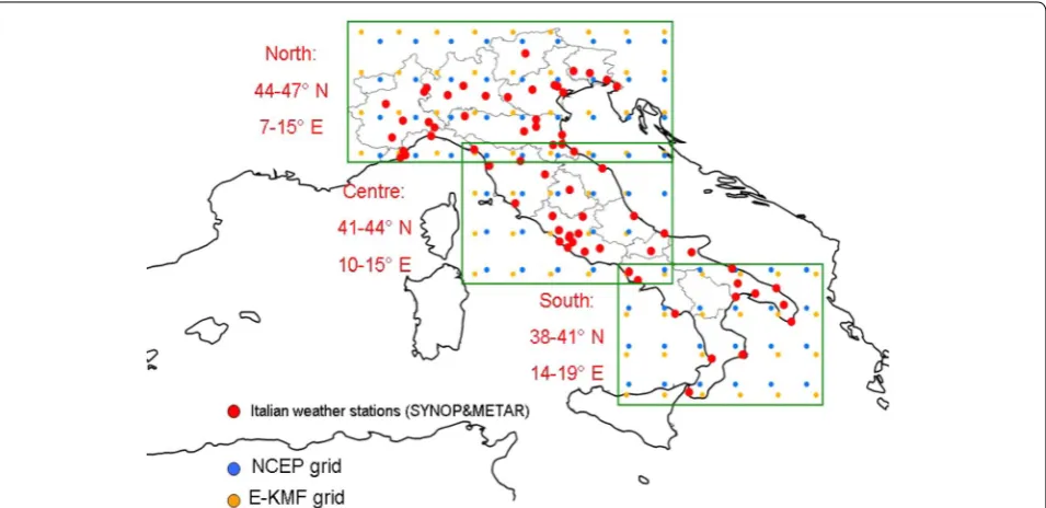
The area of study is the Italian peninsula divided into three sub-regions (macro-areas), north, centre and south (Figure 1), in order to reflect the main climate variations over the country together with the differences in energy demand. In fact, most of the north of Italy shows a humid continental climate due to the presence of the Po Valley, while a Mediterranean climate can be assigned to the central and southern Italy, as well as the coastal area of the north of the country. Moreover, the presence of the Alps and the Apennines, two important mountain chains, also plays a main role in the Italian climate. Finally, the Po Valley is the most populated and industrialized area with high energy consumptions, while central and southern Italy are less populated and show a lower energy demand.
The Kassandra Meteo forecast model
The e-kmf® global forecast system uses a multi-model and ensemble technique (Goddard et al. 2001; Mason et al. 1999) to develop the meteorological prediction of temperature from the short-medium term (typically 1–10 days) to the long-term (~2–12 weeks) forecasts (Reichler and Roads 2004). Short and medium-term fore-casts are provided by using regional and limited-area models with a grid size ranging from 5.5 km to 18 km, while long-term forecasts, as in this case study, are pro-duced using two global models with 20 perturbed initial conditions (plus one control member) each, in order to obtain a multi-model with 40 ensemble forecasts.
The first global model has a horizontal spectral triangu-lar truncation of 126 waves (T126) and 42 sigma pressure hybrid layers (L42), while the second one is a global modi-fied version of the WRF-ARW (weather research and fore-casting–advanced research WRF) model using 42 vertical levels and a horizontal grid of about 90 km. The final output of the whole ensemble is on a regular latitude-longitude grid spaced by 1°, as shown in Figure 1, with a temporal output every 6 h and a forecast horizon of 90 days. Initial condi-tions are derived from the global forecasting system (GFS) initial condition model which comes from the gridpoint sta-tistical interpolation (GSI) global data assimilation system (GDAS) and it incorporates a 3D-Var (Three Dimensional– Variational Data Assimilation) method to continuously update the background fields used for the initial condition.
The model uses global sea surface temperature (SST) boundary conditions (Reichler and Roads 2003) based on the SST anomaly simulated by a mixed-layer model. For each ensemble simulation, both the models make use of dif-ferent physical and dynamical schemes for micro-physics (Lim and Hong 2010; Hong et al. 2004), Planetary Boundary Layer and Surface Layer (Hong et al. 2006, 2008; Bretherton and Park 2009; Pleim 2006, 2007; Beljaars 1994), cumulus parameterization (Kain 2004; Han and Pan 2011), radiation (Iacono et al. 2008; Dudhia 1989; Mlawer et al. 1997), and land surface physics (Niu et al. 2011; Yang et al. 2011; Noilan and Planton 1989; Pleim and Xiu 1995).
Finally, to obtain a single value to compare with observed and climatological data in the proposed bench-mark, a selection procedure of the ensembles is applied to these two models. This selection process is applied for each time period defining a measure based on the distance between each member and the best member ensemble which is determined by using several normalized model variables; this measure is used for excluding all values outside of a defined range. The overall final value is com-puted by a weighted average of the remaining members.
The CFS‑NCEP model
The CFS-NCEP Climate Forecast System (Saha et al. 2014) was designed and executed as a global, high-reso-lution, coupled atmosphere–ocean–land surface-sea ice system. The CFS data was developed by NOAA’s National Centres for Environmental Prediction (NCEP). The data for this study are freely accessible in GRIB2 (Grid-ded Binary) format from NOAA’s National Operational Model Archive and Distribution System (NOMADS) which is stored at NOAA’s National Climatic Data Centre (NCDC).
The atmospheric model has a horizontal spectral trian-gular truncation of 126 waves (T126, equivalent to nearly a 100 km grid resolution, which is directly comparable to the resolution of e-kmf® global models), a finite differ-encing vertically with 64 sigma pressure hybrid layers, a time resolution of 6 h and a forecast horizon of 4 months which can be compared with the e-kmf forecast which has a similar overlapping period of 12 weeks as lead time. The Noah land surface model (Ek et al. 2003) is employed in the CFS in both the coupled land–atmosphere–ocean model to provide land-surface prediction of surface fluxes (surface boundary conditions), and in the global land data assimilation system (GLDAS) to provide the land surface analysis and evolving land states. For further details about this model please refer to Saha et al. (2010).
Observations and climatology
The basic temperature observation data used for both the comparison with models and the climate history regard
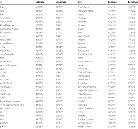
Italian weather stations and are taken from SYNOP (surface SYNOPtic observations) and METAR (METe-orological Aerodrome Report). In this study 68 weather certified stations below 500 m above sea level have been taken into account (Figure 1; Table 1). Temperatures are collected on an hourly and daily basis and stored in data base to produce all the observed data. For a long-term comparison between forecasts and observations, temper-ature data have been aggregated into weekly mean values for each reference area (north, centre and south of Italy, considering only the continental areas without the two main islands). The same weekly mean values have been used both for comparing observed and forecasted data and for arranging the climatology for each reference area. A 25-year reference period for climate data has been con-sidered (1984–2008). For each week of the year, a mean temperature value (based on 25-year data) has been obtained and used as the climatological reference for a comparison with observations and forecasts.
The benchmark analysis
Temperature forecasts produced by the two models (e-kmf® and CFS-NCEP) have been compared on the basis of statistical indexes that allow the evaluation of the performance of the two models. The aim of this study is to quantify how temperature forecasts from meteoro-logical models and climatometeoro-logical behavior perform in respect to the observed data for the three Italian macro-areas at different forecast time horizons. For both mod-els, the forecasted data are the air temperatures at 2 m above the ground on a regular latitude-longitude grid spaced by one degree (Figure 1) with a time interval of 6 h to be compared with the observed and climatologi-cal data. The benchmark analysis is performed on the forecasted data at weekly time resolution and at three macro-area spatial resolution with a forecasted horizon of 12 weeks according to the following equations that provide the macro-area weekly forecast:
(1) Tij,k,d=
1
4 4
i=1
Tj,i,d,k
(2) Ti
k
j,d = 1
5 5
k=1 Tid,j,k
(3)
Twj=
1
7 7
d=1
Ti k
j,d
(4)
Ta= 1
N N
j=1
where Tj,i,d,k is the air temperature in the grid point j for the 6 h-time interval i of the simulated day d correspond-ing to the model initialization k; Tij,k,d is the mean daily temperature of the day d in the grid point j correspond-ing to the model initialization k; Ti
k
j,d is the mean daily temperature of the day d in the grid point j averaged over the model initializations reported in Table 2; Twj is the mean weekly temperature in the grid point j; and Taj is the mean weekly temperature averaged over the N grid points within the macro-area.
Since data are available every 6 h and resolutions are not extremely high, it is more appropriate to use daily mean temperatures rather than extremes. Moreover, using several runs with different model initialization may reduce uncertainties associated with individual runs. The multi-model ensemble of the e-kmf® global forecast system may also have an improved accuracy by reducing uncertainties associated with individual models. The same procedure (Figure 2) used for the e-kmf® model data output is applied for the CFS-NCEP model.
Table 1 Italian weather stations below 500 m a.s.l. used for observed data of the year 2010 and for the climatological mean (1984–2008)
Site Latitude Longitude Site Latitude Longitude
Bolzano 46°28′N 11°20′E Pisa/S. Giusto 43°41′N 10°23′E
Aviano 46°02′N 12°36′E Firenze/Peretola 43°48′N 11°12′E
Udine 45°59′N 13°02′E Arezzo 43°28′N 11°51′E
Torino/Caselle 45°13′N 7°39′E Perugia 43°05′N 12°30′E
Novara/Cameri 45°31′N 8°40′E Falconara 43°37′N 13°22′E
Milano/Malpensa 45°37′N 8°44′E Grosseto 42°45′N 11°04′E
Bergamo/Orio Al Serio 45°40′N 9°42′E Viterbo 42°26′N 12°03′E
Milano/Linate 45°26′N 9°17′E Rieti 42°25′N 12°51′E
Piacenza 44°55′N 9°44′E Vigna Di Valle 42°05′N 12°13′E
Brescia/Ghedi 45°25′N 10°17′E Pescara 42°26′N 14°12′E
Verona/Villafranca 45°23′N 10°52′E Termoli 42°00′N 15°00′E
Vicenza 45°34′N 11°31′E Guidonia 42°00′N 12°44′E
Treviso/Istrana 45°41′N 12°06′E Roma/Urbe 41°57′N 12°30′E
Treviso/S. Angelo 45°39′N 12°11′E Roma/Ciampino 41°47′N 12°35′E
Trieste 45°39′N 13°45′E Roma 41°54′N 12°29′E
Venezia/Tessera 45°30′N 12°20′E Roma Fiumicino 41°48′N 12°14′E
Ronchi Dei Legionari 45°49′N 13°29′E Latina 41°33′N 12°54′E
Trieste 45°39′N 13°45′E Frosinone 41°38′N 13°18′E
Mondovì 44°23′N 7°49′E Pratica Di Mare 41°39′N 12°27′E
Govone 44°48′N 8°06′E Campobasso 41°34′N 14°39′E
Novi Ligure 44°46′N 8°47′E Grazzanise 41°03′N 14°04′E
Passo Dei Giovi 44°38′N 8°56′E Amendola 41°32′N 15°43′E
Genova/Sestri 44°25′N 8°51′E Bari/Palese Macchie 41°08′N 16°47′E
Albenga 44°03′N 8°07′E Napoli/Capodichino 40°51′N 14°18′E
Sarzana/Luni 44°05′N 9°59′E Capo Palinuro 40°01′N 15°17′E
Ferrara 44°50′N 11°37′E Gioia Del Colle 40°46′N 16°56′E
Bologna/Borgo Panigale 44°32′N 11°18′E Brindisi 40°39′N 17°57′E
S. Pietro Capofiume Bologna 44°39′N 11°37′E Grottaglie 40°31′N 17°24′E
Punta Marina 44°27′N 12°18′E Marina Di Ginosa 40°26′N 16°53′E
Forlì 44°12′N 12°04′E Lecce 40°14′N 18°09′E
Cervia 44°13′N 12°18′E Crotone 39°00′N 17°04′E
Rimini 44°02′N 12°37′E S. Maria Di Leuca 39°49′N 18°21′E
Capo Mele 43°57′N 8°10′E Lamezia Terme 38°54′N 16°15′E
Data analysis
Different statistical performances are used to understand the predictability and reliability of temperature forecasts
for each month in a perspective of 12 weeks ahead. The statistical analysis is computed for both forecast models and climatology mean (based on 1984–2008 data), by comparing them to the observations for each month of 2010. The indexes used and discussed in the following section are: the forecast error (FE) at given observed tem-perature values, the mean absolute error (MAE), the cli-matological Skill Score (SSclim), the anomaly correlation coefficient (ACC).
The forecasted error
The calculated forecasted error (Eq. 5) for each observed data is:
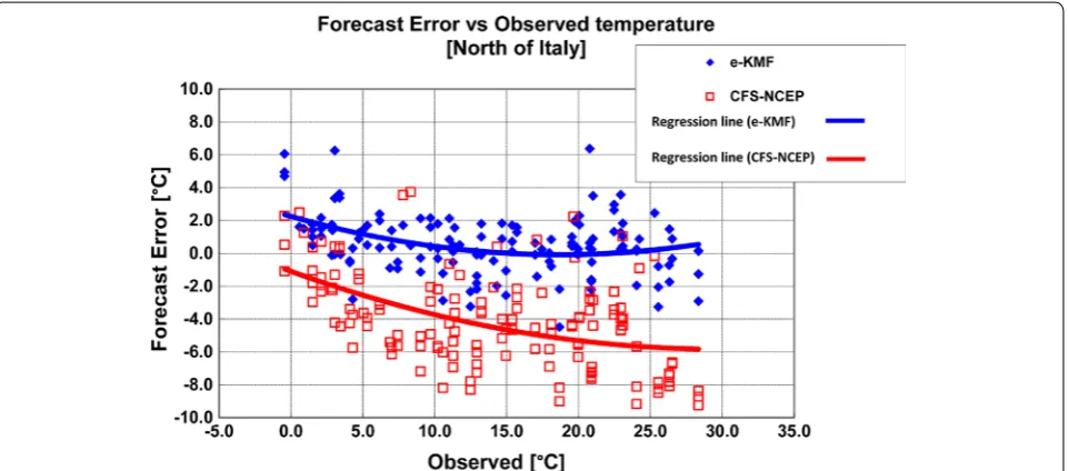
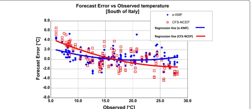
where: Oi = observed value; Fi = forecasted value. Figures 3, 4, and 5 show the forecasting error in com-parison with observed values for all the forecasted weeks of the year for the north, centre and south of Italy, respec-tively. These plots are used to illustrate the errors between forecasts and observation data according to a given tem-perature; in this way, we are able to control possible under/ overestimation of the model depending on temperature
(5) FEi=Fi−Oi
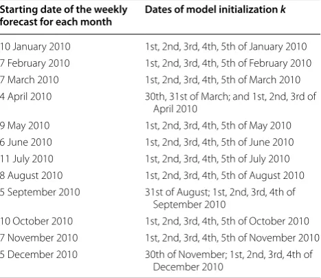
Table 2 Starting date of the weekly forecast for each ana-lyzed month of the year 2010
Starting date of the weekly
forecast for each month Dates of model initialization k
10 January 2010 1st, 2nd, 3rd, 4th, 5th of January 2010 7 February 2010 1st, 2nd, 3rd, 4th, 5th of February 2010 7 March 2010 1st, 2nd, 3rd, 4th, 5th of March 2010 4 April 2010 30th, 31st of March; and 1st, 2nd, 3rd of
April 2010
9 May 2010 1st, 2nd, 3rd, 4th, 5th of May 2010 6 June 2010 1st, 2nd, 3rd, 4th, 5th of June 2010 11 July 2010 1st, 2nd, 3rd, 4th, 5th of July 2010 8 August 2010 1st, 2nd, 3rd, 4th, 5th of August 2010 5 September 2010 31st of August; 1st, 2nd, 3rd, 4th of
September 2010
10 October 2010 1st, 2nd, 3rd, 4th, 5th of October 2010 7 November 2010 1st, 2nd, 3rd, 4th, 5th of November 2010 5 December 2010 30th of November; 1st, 2nd, 3rd, 4th of
December 2010
Figure 2 Diagram of each step of the procedure for calculating the weekly temperature forecast T(ai); Ini date is the date of the forecast
values and it is possible to evaluate the performance of the forecasting model in different climate seasons.
Figure 3 highlights how the CFS-NCEP model underes-timates temperature forecasts in the north of Italy (about 4°C), while only a slight overestimation is provided by the e-kmf® model.
On the contrary, for the centre of Italy, the CFS-NCEP model shows an overestimation of temperature forecasts with values of less than 10°C (colder months)
and an underestimation for temperatures greater than 10°C (warmer months); a similar trend, although less enhanced, was found for the e-kmf® model (Figure 4).
In the south of Italy, there is a significant temperature forecast overestimation below 12–13°C and an underesti-mation above 23°C by the CFS-NCEP model. The e-kmf® model shows an overestimation when the observed tem-peratures are under 10°C and no errors greater than ±3°C for warmer temperature values (Figure 5).
Figure 3 Forecast error vs. observed temperature values for the e-kmf® (blue rhombi) and the CFS-NCEP (red squares) model in the north of Italy; the two polynomial regressions are shown with a blue and red line, respectively for the e-kmf® and CFS-NCEP model.
The mean absolute error
The MAE for the three macro-areas is shown in Tables 3 and 4 and calculated as follows (Eq. 6):
where Oi = observed value; Fi = forecasted or climato-logical value, n = numbers of analyzed data.
The computed values show lower errors for the macro-area of centre and south of Italy for the two meteoro-logical models and climatometeoro-logical data. For the northern
(6)
MAE = 1
n
n
i=1
|Fi−Oi|
macro-area, the CFS-NCEP model highly underestimates the forecasted temperatures.
The reason for a lower MAE in the centre and south macro-area can be related to the forecast predictability which is higher in these two areas than in the northern one where the orography plays a relevant role; in fact, as it is shown in Figure 1, most of the grid points in south-ern area are over the sea surface and the topography is smoother than in the north. In addition to this first com-parison, the MAE has been calculated as a mean of the ith weekly forecast of the 12 months in order to under-stand the reliability of forecast horizon for each model
Figure 5 Forecast error vs. observed temperature values for the e-kmf® (blue rhombi) and the CFS-NCEP (red squares) model in the south of Italy; the two polynomial regressions are shown with a blue and red line, respectively for the e-kmf® and CFS-NCEP models.
Table 3 Mean absolute error of temperature (°C) for each model (e-kmf®, CFS-NCEP, Climatology) vs. area and month
Initialization month e‑kmf® Climatology CFS‑NCEP
North Center South North Center South North Center South
January 1.25 0.92 0.69 1.77 1.86 1.58 4.01 2.56 2.39
February 1.80 1.61 1.23 1.84 2.05 1.66 5.29 2.75 1.62
March 1.46 1.24 0.99 1.90 1.66 1.44 6.03 2.42 1.54
April 0.99 0.75 0.66 1.78 1.57 1.60 5.88 2.36 1.81
May 1.58 1.67 1.74 2.26 2.14 1.65 6.35 2.78 1.85
June 1.05 0.68 0.90 2.30 2.15 1.60 5.42 2.57 1.90
July 1.46 1.24 0.99 1.90 1.66 1.44 5.10 2.12 1.40
August 0.86 0.61 0.47 1.41 1.18 1.05 4.23 1.71 1.39
September 0.95 0.56 0.43 1.31 1.15 0.89 5.05 2.01 1.11
October 1.97 1.46 1.57 2.10 1.59 1.66 2.96 1.91 2.18
November 1.57 1.43 1.40 1.78 1.52 1.48 2.43 1.31 2.53
December 1.69 1.48 2.09 1.90 1.65 1.55 3.40 1.29 2.66
and macro-area. As can be seen from Table 4, the best score is obtained by the e-kmf® model in the first fore-casting week, with a worsening of the performance between the 5th and 8th forecasting week as shown in Table 5 and Figure 3 as well. Table 6 shows the percent-age of cases where the MAE of the temperature forecast is in selected ranges. These percentages have been com-puted on four classes: 0–1°C, 1–2°C, 2–4°C and >4°C. A MAE in the first two classes (between 0 and 1°C and 1–2°C) can be considered an excellent or good result, respectively, in terms of weekly prediction; the third class with forecast errors between 2 and 4°C may be considered a fair to a rather poor result and, finally, an
error above 4°C may be considered a poor or a very poor achievement.
In particular, the e-kmf® model obtains a good per-formance: only 4% of the cases with a forecasting error above 4°C, while the CFS-NCEP model results were less satisfactory, especially in northern Italy, where 60% of the cases has a MAE above 4°C.
The climatological Skill Score
One of the most important scores used to evaluate the performance is the SSclim, which gives an idea of the relative improvement (or worsening) of the forecast-ing model in relation to certain reference values; the
Table 4 Mean absolute error of temperature (°C) for each week of forecasting between the e-kmf® and the CFS-NCEP model for each area of Italy
Week of forecast e‑kmf Climatology CFS‑NCEP
North Centre South North Centre South North Centre South
1 0.89 0.53 1.42 0.00 0.22 0.96 22.62 4.05 4.72
2 3.41 2.14 2.91 7.76 2.04 3.83 23.37 5.88 7.86
3 3.13 3.95 2.25 11.90 1.94 0.63 27.56 8.03 5.06
4 3.88 2.44 1.79 5.69 2.14 1.15 31.27 6.85 3.83
5 4.53 3.63 2.97 3.97 4.09 1.69 26.38 6.50 4.90
6 3.97 3.11 3.21 0.22 4.44 4.93 29.33 8.65 7.57
7 6.62 6.52 3.82 0.96 12.60 5.59 28.81 7.80 3.03
8 4.89 1.68 3.21 0.24 1.84 1.54 25.00 4.40 3.30
9 2.06 0.91 1.50 28.55 11.46 7.06 29.13 6.69 3.32
10 5.05 4.10 2.75 0.05 0.17 1.16 26.97 6.73 7.41
11 1.09 0.85 1.50 6.18 7.41 3.24 30.88 7.11 3.33
12 2.29 1.20 0.94 0.34 3.94 2.10 27.28 6.74 8.03
Mean 3.48 2.59 2.36 5.49 4.36 2.82 27.38 6.62 5.20
Table 5 ACC values for the e-kmf® and CFS-NCEP models for ith forecasting week in the three macro-areas
Week of forecast e‑kmf® CFS‑NCEP
North Centre South North Centre South
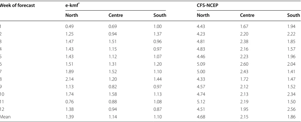
1 0.49 0.69 1.00 4.43 1.67 1.94
2 1.25 0.94 1.37 4.23 2.20 2.22
3 1.47 1.51 0.96 4.81 2.38 1.85
4 1.43 1.15 0.97 4.83 2.16 1.57
5 1.43 1.12 1.07 4.46 2.23 1.96
6 1.51 1.31 1.20 5.09 2.60 2.04
7 1.89 1.52 1.10 5.00 2.43 1.41
8 2.14 1.20 1.44 4.33 1.72 1.47
9 1.13 0.82 0.97 4.57 2.12 1.52
10 1.74 1.58 1.13 4.74 2.13 2.34
11 0.76 0.88 1.08 5.12 2.19 1.50
12 1.38 0.94 0.87 4.51 1.95 2.56
climatological mean has been used in this case study. The SS is calculated as follows (Eq. 7):
where the MSE forecast, clim, and obs are the mean square error for the forecasted, climatological and observed data respectively and the MSE equation is cal-culated as follows (Eq. 8):
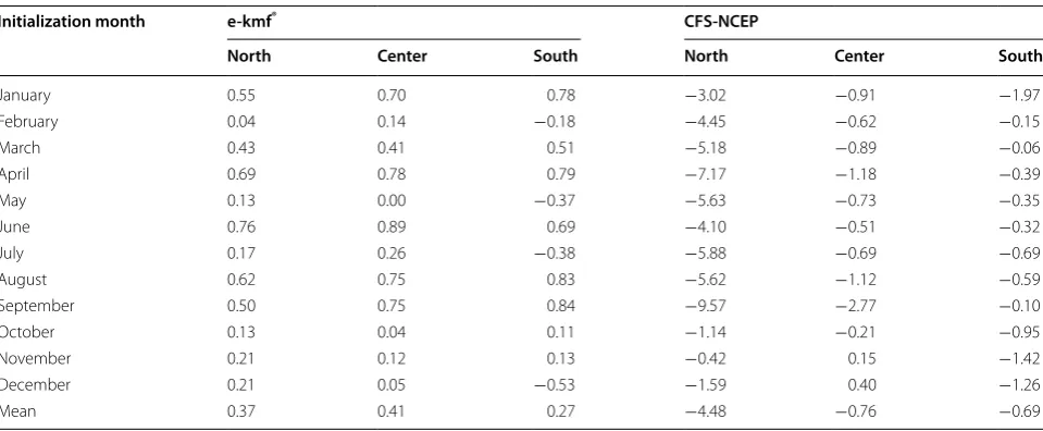
As it is shown in Table 7, using the e-kmf® model there is a huge improvement for almost all months and for all areas: the three scores for the north, centre and south of Italy give an average improvement of 35% for the year 2010; this means that the e-kmf® model increases fore-casting capability, with better forefore-casting results for 2-m air temperature of 35%, compared to the climatological averages. On the contrary, the CFS-NCEP model shows (7) SSclim = MSEforecast−MSEclim
MSEobs− MSEclim
=1−MSEforecast MSEclim
(8)
MSE = 1
n
n
i−1
(Fi−Oi)2
the opposite for almost all months and all areas, meaning that it would be better to use climatology to estimate sea-sonal temperature trends for the following weeks instead of the forecasting model.
The anomaly correlation coefficient
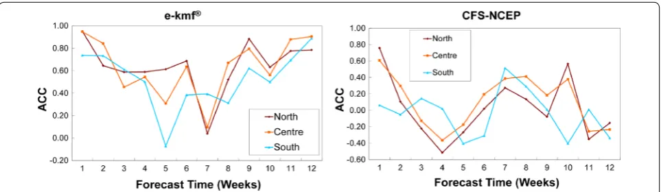
Another important score is the ACC which gives an idea of the correlation between models and observed data, subtracting the climatological mean. In fact, another way to measure the quality of a forecasting system is to calcu-late the correlation between forecasts and observations. However, correlating forecasts directly with observations or analyses may give misleadingly high values, due to sea-sonal variations. It is therefore an established practice to subtract the climate average from both the forecast and the verification and to assess the forecast and observed anomalies according to the ACC.
The ACC is calculated as follows:
(9) ACC =
n i=1
(Fi−Ci)−(F−C)·(Oi−Ci)−(O−C)
n
i=1
(Fi−Ci)−(F−C)
2 ·
(Oi−Ci)−(O−C)
2 Table 6 Percentage of cases where the mean absolute error of temperature forecasting is between 0–1°C, 1–2°C, 2–4°C and above 4°C for each area between the e-kmf® and CFS-NCEP models and the climatological mean for the year 2010 Mean absolute error
of temperature forecast (%) e‑KMF Climatology NCEP
North Centre South North Centre South North Centre South
between 0–1°C 47.92 59.03 59.72 36.81 30.56 33.33 4.86 25.00 29.86
between 1–2°C 29.86 25.69 25.69 24.31 40.28 39.58 7.64 29.86 29.17
between 2–4°C 17.36 11.11 11.11 29.86 25.69 25.00 27.78 31.25 34.72
between >4°C 4.86 4.17 3.47 9.03 3.47 2.08 59.72 13.89 6.25
Table 7 Climatological Skill Scores for the two models (e-kmf®, CFS-NCEP) and for each area and month
Initialization month e‑kmf® CFS‑NCEP
North Center South North Center South
January 0.55 0.70 0.78 −3.02 −0.91 −1.97
February 0.04 0.14 −0.18 −4.45 −0.62 −0.15
March 0.43 0.41 0.51 −5.18 −0.89 −0.06
April 0.69 0.78 0.79 −7.17 −1.18 −0.39
May 0.13 0.00 −0.37 −5.63 −0.73 −0.35
June 0.76 0.89 0.69 −4.10 −0.51 −0.32
July 0.17 0.26 −0.38 −5.88 −0.69 −0.69
August 0.62 0.75 0.83 −5.62 −1.12 −0.59
September 0.50 0.75 0.84 −9.57 −2.77 −0.10
October 0.13 0.04 0.11 −1.14 −0.21 −0.95
November 0.21 0.12 0.13 −0.42 0.15 −1.42
December 0.21 0.05 −0.53 −1.59 0.40 −1.26
where: Oi, Fi, and C are the observed, forecasted and climatological values are the average values of the dif-ferences between observations or forecasts and climato-logical values for the analyzed data set. n = number of analyzed data.
Table 5 and Figure 6 (left) show how the e-kmf® model has a higher reliability for the first and third forecast-ing month (i.e. from the 1st to the 4th forecastforecast-ing week and from the 9th to the 12th). On the contrary there is a worsening for the e-kmf® forecast in the 2nd month (i.e. from the 5th to the 8th week). For the CFS-NCEP model there is no general trend and very low values of ACC are shown in Figure 6 (right), i.e. no correlation at all between this model and observed data for every forecast-ing week, except for the first one.
Conclusions
Reliable meteorological forecasting in specific geographic areas could be a suitable support for improving opera-tions in the energy market. A lot of progress has been made in the development of meteorological models and downstream applications, as well as forecast planning in gas and power supply and renewable energy generation in the last decade. From a long-term perspective, a mete-orological seasonal forecast, which is often based on cli-matology, will be able to provide capability management in a time scale of just a few months.
As a major energy company, with the aim of improving the commercial planning of oil, natural gas and power, Eni has developed the kassandra meteo forecast (e-kmf®) model, i.e. a short to long term (from 1 to 90 days) pro-prietary meteorological forecast system in collaboration with the Epson Meteo centre. These new numerical mod-els for temperature forecasting trends provide an alterna-tive solution to statistical systems based on climatological data analysis. The e-kmf® meteorological model is based on the probabilistic approach of the ensemble technique and it will be used for energy resource management in
different European regions. In fact, an accuracy improve-ment of forecasted temperature by about 1°C compared to values obtained by climatology may have a great ben-efit in gas supply portfolio management.
In this paper we evaluated the long-term tempera-ture forecast performance of the e-kmf® and CFS-NCEP models in three regions in Italy (north, centre and south, excluding the main Italian islands) for the entire year 2010.
In particular, daily temperature forecasts collected from five daily initialization runs were averaged out to obtain a weekly forecast for each model grid point related to the three Italian macro-areas; afterwards, each tem-perature forecast of the model grid point was once again averaged in order to obtain a single temperature forecast value for each week (12 in total for each area). Statisti-cal indexes have been used to Statisti-calculate the performance analysis by comparing the observed data, the climatologi-cal mean and the two models that were analyzed.
According to the MAE the e-kmf® model performs bet-ter than the CFS-NCEP model in almost all areas and forecast initialization months. The SSclim index shows how the e-kmf® model has an average improvement of 35% compared with climatology (used as a reference) for the year 2010, while the performance of the CFS-NCEP is worse, in particular in the northern Italian macro-area where there is a significant mean underestimation (4.7°C using the mean absolute error).
The ACC provides information that is very useful for understanding the reliability of the forecast from the 1st to the 12th week for each forecast initialization month. In particular, the e-kmf® model shows a good correlation between forecasted and observed temperature data in the 1st and 3rd month of the forecast, while a worsening of the model’s performance was observed between the 5th and 8th week of prediction. This particular aspect will be investigated in more detail in order to improve the fore-cast for the entire period analyzed.
Abbreviations
3D-Var: three-dimensional variational data assimilation; ACC: anomaly cor-relation coefficient; CCGT: combined-cycle gas turbine; CDD: cooling degree day; CFS-NCEP: Climate Forecast System–National Centers for Environmental Prediction; CHP: combined heat and power; e-kmf®: eni-kassandra meteo forecast; FE: forecast error; GDAS: global data assimilation system; GFS: global forecasting system; GLDAS: global land data assimilation system; GSI: gridpoint statistical interpolation; HDD: heating degree day; MAE: mean absolute error; METAR: METeorological Aerodrome Report; MSE: mean square error; NCDC: National Climatic Data Centre; NOAA: National Oceanic and Atmospheric Administration; NOMADS: National operational model archive and distribution system; SSclim: climatological Skill Score; SST: sea surface temperature; SYNOP: surface SYNOPtic observations; WRF-ARW: weather research and forecasting– advanced research WRF.
Author’s contribution
AC worked on the benchmark analysis and data interpretation and he wrote most of the manuscript. GG wrote the background introduction and purposes of the paper. He presented an oral presentation regarding this study at the AOGS 2013 in Brisbane. RS developed the e-kmf model, collected all observed and climate data, and supervised all simulations of the model. GE has been involved in data model analysis and debugging. MM supervised the complete manuscript for important intellectual content and approved it for the final ver-sion to be published. All authors read and approved the final manuscript.
Author details
1 eni S.p.A. Midstream Department, San Donato Milanese, Italy. 2 Epson Meteo Centre, Sesto S. Giovanni, Italy. 3 Department of Civil and Environmental Engi-neering, Politecnico di Milano, Milan, Italy.
Acknowledgements
This research was carried out as part of the METEO Project funded by Eni. The authors are grateful to Dr. Michela Giorgetti and Dr. Roberto Vernazza for a fruitful scientific discussion.
Compliance with ethical guidelines
Competing interests
The authors declare that they have no competing interests (both financial and non-financial ones).
Received: 11 December 2014 Accepted: 8 June 2015
References
Alexiadis MC, Dokopoulos PS, Sahsamanoglou HS, Manousaridis IM (1998) Short-term forecasting of wind speed and related electrical power. Sol Energy 63(1):61–68
Beljaars ACM (1994) The parameterization of surface fluxes in large-scale mod-els under free convection. Q J R Meteorol Soc 121:255–270
Bretherton CS, Park S (2009) A new moist turbulence parameterization in the Community Atmosphere Model. J Clim 22:3422–3448
Carvalho D, Rocha A, Gómez-Gesteira M, Silva Santos C (2014) WRF wind simula-tion and wind energy producsimula-tion estimates forced by different reanalyses: comparison with observed data for Portugal. Appl Energy 117:116–126 Cassola F, Burlando M (2012) Wind speed and wind energy forecast through
Kalman filtering of numerical weather prediction model output. Appl Energy 99:154–166
Cox JD (2002) Storm watchers: the turbulent history of weather prediction from Franklin’s kite to El Niño. Wiley, New York
Dovrtel K, Medved S (2011) Weather-predicted control of building free cooling system. Appl Energy 88(9):3088–3096
Dudhia J (1989) Numerical study of convection observed during the winter monsoon experiment using a mesoscale two-dimensional model. J Atmos Sci 46:3077–3107
Ek M, Mitchell KE, Lin Y, Rogers E, Grunmann P, Koren V et al (2003) Implemen-tation of Noah land-surface model advances in the NCEP operational mesoscale Eta model. J Geophys Res 108(D22):8851. doi:10.1029/200 2JD003296
Forouzanfar M, Doustmohammadi A, Menhaj MB, Hasanzadeh S (2010) Mod-eling and estimation of the natural gas consumption for residential and commercial sectors in Iran. Appl Energy 87(1):268–274
Franco F, Sanstad AH (2008) Climate change and electricity demand in Califor-nia. Clim Change 87(1):139–151
Giorgetti M, Giunta G, Salerno R, Vernazza R (2012) Medium-long term meteorological forecasting method and system. WO Patent App. PCT/ IB2011/055632, WO 2012/080944 A1
Giunta G, Salerno R (2013) Short-long term temperature forecasting method and system for production management and sale of energy resources. WO Patent App. PCT/IB2013/0546780, WO 2013/186703 A1
Goddard L, Mason SJ, Zebiak SE, Ropelewski CF, Basher R, Cane MA (2001) Current approaches to seasonal-to-interannual climate predictions. Int J Climatol 21(9):1111–1152
Gorucu FB, Gumrah F (2004) Evaluation and forecasting of gas consumption by statistical analysis. Energy Sour 26(3):267–276
Han J, Pan H-L (2011) Revision of convection and vertical diffusion schemes in the NCEP global forecast system. Weather Forecast 26:520–533 Hong S-Y, Dudhia J, Chen S-H (2004) A revised approach to ice microphysical
processes for the bulk parameterization of clouds and precipitation. Mon Weather Rev 132:103–120
Hong S-Y, Noh Y, Dudhia J (2006) A new vertical diffusion package with an explicit treatment of entrainment processes. Mon Weather Rev 134:2318–2341
Hong S-Y, Choi J, Chang E-C, Park H, Kim Y-J (2008) Lower-tropospheric enhancement of gravity wave drag in a global spectral atmospheric forecast model. Weather Forecast 23:523–531
Iacono MJ, Delamere JS, Mlawer EJ, Shephard MW, Clough SA, Collins WD (2008) Radiative forcing by long-lived greenhouse gases: calculations with the AER radiative transfer models. J Geophys Res 113:D13103 Isaac M, van Vuuren DP (2009) Modeling global residential sector energy
demand for heating and air conditioning in the context of climate change. Energy Policy 37(2):507–521
Jolliffe IT, Stephenson DB (eds) (2003) Forecast verification: a practitioner’s guide in atmospheric science. Wiley, New York
Kain JS (2004) The Kain-Fritsch convective parameterization: an update. J Appl Meteorol 43:170–181
Leviäkangas P, Hautala R (2009) Benefits and value of meteorological informa-tion services—the case of the Finnish Meteorological Institute. Meteorol Appl 16(3):369–379
Lim K-SS, Hong S-Y (2010) Development of an effective double-moment cloud microphysics scheme with prognostic cloud condensation nuclei (CCN) for weather and climate models. Mon Weather Rev 138:1587–1612 Mason SJ, Goddard L, Graham NE, Yulaeva E, Sun L, Arkin PA (1999) The IRI
seasonal climate prediction system and the 1997/98 El Niño event. Bull Am Meteorol Soc 80(9):1853–1873
Mirasgedis S, Sarafidis Y, Georgopoulou E, Lalas DP, Moschovits M, Karagian-nis F et al (2006) Models for mid-term electricity demand forecasting incorporating weather influences. Energy 31(2):208–227
Mlawer EJ, Taubman SJ, Brown PD, Iacono MJ, Clough SA (1997) Radiative transfer for inhomogeneous atmospheres: RRTM, a validated correlated-k model for the longwave. J Geophys Res 102:16663–16682
Niu G-Y, Yang Z-L, Mitchell KE, Chen F, Ek MB, Barlage M et al (2011) The com-munity Noah land surface model with multiparameterization options (Noah-MP): 1. Model description and evaluation with local–scale meas-urements. J Geophys Res 116. Art. ID D12109. doi:10.1029/2010JD015139 Noilan J, Planton S (1989) A simple parameterization of land surface processes
for meteorological models. Mon Weather Rev 117:536–549 Oldewurtel F, Parisio A, Jones CN, Gyalistras D, Gwerder M, Stauch V et al
(2012) Use of model predictive control and weather forecasts for energy efficient building climate control. Energy Build 45:15–27
Palmer T, Hagedorn R (eds) (2006) Predictability of weather and climate. Cam-bridge University Press, CamCam-bridge
Petersen S, Bundgaard KW (2014) The effect of weather forecast uncertainty on a predictive control concept for building systems operation. Appl Energy 116:311–321
Pinson P, Nielsen HA, Madsen H, Kariniotakis G (2009) Skill forecast-ing from ensemble predictions of wind power. Appl Energy 86(7):1326–1334
Pleim JE (2007) A Combined local and nonlocal closure model for the atmospheric boundary layer. Part I: model description and testing. J Appl Meteorol Climatol 46:1383–1395
Pleim JE, Xiu A (1995) Development and testing of a surface flux and planetary boundary layer model for application in mesoscale models. J Appl Meteorol 34:16–32
Potocnik P, Thaler M, Govekar E, Grabec I, Poredos A (2007) Forecasting risks of natural gas consumption in Slovenia. Energy Policy 35(8):4271–4282 Reichler TJ, Roads JO (2003) The role of boundary and initial conditions for
dynamical seasonal predictability. Nonlinear Process Geophys 10:1–22 Reichler TJ, Roads JO (2004) Time-space distribution of long-range
atmos-pheric predictability. J Atmos Sci 61(3):249–263
Saha S, Moorthi S, Pan HL, Wu X, Wang J, Nadiga S et al (2010) The NCEP cli-mate forecast system reanalysis. Bull Am Meteorol Soc 91(8):1015–1057. doi:10.1175/2010BAMS3001.1
Saha S, Moorthi S, Wu X, Wang J, Nadiga S, Tripp P et al (2014) The NCEP climate forecast system version 2. J Clim 27(6):2185–2208
Sánchez-Úbeda EF, Berzosa A (2007) Modeling and forecasting industrial end-use natural gas consumption. Energy Econ 29(4):710–742
Smith P, Husein S, Leonard DT (1996) Forecasting short term regional gas demand using an expert system. Expert Syst Appl 10(2):265–273 Soldo B (2012) Forecasting natural gas consumption. Appl Energy 92:26–37 Vidrih B, Medved S (2008) The effects of changes in the climate on the energy
demands of buildings. Int J Energy Res 32(11):1016–1029
Wilks DS (2006) Statistical methods in the atmospheric sciences. Academic Press, New York
WWRP/WGNE Joint working group on forecast verification research. Forecast verification—issue, methods and FAQ. http://www.cawcr.gov.au/pro-jects/verification. Accessed 26 January 2015
Yang Z-L, Niu G-Y, Mitchell KE, Chen F, Ek MB, Barlage M et al (2011) The com-munity Noah land surface model with multiparameterization options (Noah-MP): 2. Evaluation over global river basins. J Geophys Res 116. Art. ID D12110. doi:10.1029/2010JD015140