A local adaptive refinement method with multigrid preconditionning illustrated by multiphase flows simulations.

C. Besse, O. Goubet, T. Goudon & S. Nicaise, Editors

A LOCAL ADAPTIVE REFINEMENT METHOD WITH MULTIGRID

PRECONDITIONNING ILLUSTRATED BY MULTIPHASE FLOWS

SIMULATIONS.

Franck Boyer

, Celine Lapuerta

, Sebastian Minjeaud

and Bruno Piar

Abstract. The aim of this paper is to describe some numerical aspects linked to incompressible three-phase flow simulations, thanks to Cahn-Hilliard type model. The numerical capture of transfer phenomenon in the neighborhood of the interface require a mesh thickness which become crippling in the case where it is applied to the whole computational domain. This suggests the use of a local refinement method which allows to dynamically focus on problematic areas. The notion of refinement pattern, introduced for Lagrange finite elements, allows to build a conceptual hierarchy of nested con-formal approximation spaces which is then used to implement the so-called CHARMS local refinement methods. Properties of these methods are proved ensuring in particular the conformity of approxi-mation spaces at every time of simulations. Furthermore, the multilevel structure obtained by this method, is used to construct multigrid preconditioners. Finally, after a validation on a model problem, the performance of the whole method is illustrated on an example of a liquid lens spreading between two stratified fluids.

R´esum´e. L’objectif de l’article est de d´ecrire certains aspects num´eriques li´es `a la simulation d’´ ecou-lements incompressibles `a trois phases non miscibles, `a l’aide de mod`eles `a interfaces diffuses de type Cahn-Hilliard. La capture num´erique des ph´enom`enes de transfert au voisinage des interfaces requiert une finesse de maillage qui devient r´edhibitoire si elle est appliqu´ee `a l’ensemble du domaine de calcul. Ceci sugg`ere l’utilisation de m´ethodes de raffinement local adaptatif qui permettent de se focaliser dy-namiquement sur les zones sensibles. La notion de motif de raffinement, introduite pour des ´el´ements finis de Lagrange, permet de construire une hi´erarchie conceptuelle d’espaces d’approximation con-formes emboˆıt´es qui est alors utilis´ee pour mettre en oeuvre les techniques de raffinement local dites CHARMS. Les propri´et´es de la m´ethode sont prouv´ees assurant en particulier la conformit´e de l’espace d’approximation `a tout instant des simulations. En outre, la structure multiniveaux obtenue par cette m´ethode est exploit´ee pour construire des pr´econditionneurs multigrilles. Enfin, apr`es une validation sur un probl`eme mod`ele, les performances de l’ensemble sont illustr´ees sur un exemple d’´etalement d’une lentille pi´eg´ee entre deux phases stratifi´ees.

1_{Laboratoire d’Analyse, Topologie et Probabilit´es (LATP), Facult´e des Sciences et Techniques de Saint-J´erˆome - Case Cour A,}

Universit´e Paul C´ezanne, Avenue Escadrille Normandie-Niemen, 13397 MARSEILLE Cedex 20, France. e-mail:[email protected]

2 _{Institut de Radioprotection et de Sˆuret´e Nucl´eaire (IRSN), DPAM/SEMIC/LIMSI, BP-3, 13115 Saint-Paul-lez-Durance,}

France.

e-mail:[email protected] & [email protected] & [email protected]

c

EDP Sciences, SMAI 2009

Contents

Introduction 16

1. Multilevel Finite Element Spaces 18

1.1. Preliminary notation and definitions 18

1.2. Refinement pattern 20

1.3. Multilevel finite element approximation spaces 22

2. Adaptation procedure and multigrid preconditioners 28

2.1. Adaptation 28

2.2. Multigrid preconditioner 34

2.3. Validation on a stationnary model problem 38

3. Application to a ternary Cahn-Hilliard system 41

3.1. Introduction 41

3.2. Discretization procedure 44

3.3. Practical issues 46

3.4. Numerical experiments 49

4. Conclusion 51

References 52

Introduction

During a hypothetical major accident in a nuclear reactor, the degradation of the core may produce multiphase flows where interfaces undergo extreme topological changes, e.g. break-up and coalescence. Because of their ability to capture interfaces implicitly, phase field models are attractive for the numerical simulation of such phenomena [5]. They replace sharp interfaces by thin but nonzero thickness transition regions where capillary effects and changes in fluid properties are smoothed. The implied burden on the numerical method lies in the required resolution of very thin moving internal layers. We present here a general adaptive local refinement strategy and an associated multigrid solver in order to tackle such issues. We illustrate the method on the ternary Cahn-Hilliard model taken from [5].

The challenge of local refinement can be expressed in that way: increase the spatial resolution of some part of the domain which are dynamically selected at each time step. Of course, the choice of these parts is not obvious, nevertheless, for the description of the general method, we assume that a refinement criterion is available so that we know the area to refine. We will give, in Section 3.3.3, the precise criterion we used for the resolution of the Cahn-Hilliard model.

To increase the spatial resolution in these selected areas, a solution is to use elements with smaller diameters, i.e. to split some cells into smaller ones. The main difficulty is to preserve, at the same time, the geometric conformity of the mesh and then its “good” geometric quality. The geometric conformity prevents the so-called hanging nodes which for different reasons are undesired in many applications. For instance, hanging nodes do not represent degree of freedom and are somewhat difficult to handle, because the local correlation pattern of the stiffness matrix is disturbed. When they exist, their taking into account may be carried out by many ways, for instance, by direct elimination of these “false” unknowns, or by adding constraint and using penalty methods or Lagrange multiplier methods. In these cases, numerical methods and schemes are modified.

corner. This yields a simple bisection which is “irregular” but only used for solving conformity issues. Bey [4] and Zhang [24] proposed a generalisation of this method to three dimensions. Other methods based only on bisection have been introduced by Rivara [21, 22] or Mitchell [18] in two dimension and B¨ansch [3] or Maubach [17] in three dimensions. All these methods depend on the choice of the element and on the dimension. Moreover, their implementation tends to be quite complex, notably in three dimensions.

A possible alternative considered in this paper is to adopt the point of view of basis functions refinement instead of cells refinement. In this approach [15], a stock of basis functions with increasing spatial resolution is assumed to be given through a nested sequence of approximation spaces X0 ⊂ · · · ⊂ XJ, J > 1. Local

refinement is then performed by using multilevel approximation spaces containing few basis functions suitably selected in each approximation spacesXj, j∈J0, JK. In this framework, Krysl, Grinspun and Schr¨oder in [15]

(see also [10, 13, 16]) proposed procedures called CHARMS (Conforming Hierarchical Adaptive Refinement MethodS) which enable to (un)refine multilevel approximation spaces. We give here a precise construction of the nested sequence X0 ⊂ · · · ⊂ XJ for suitable Lagrange finite element (e.g. Pk,Qk, k >1) using a unique

refinement pattern and we study a slightly modified version of the quasi-hierarchical CHARMS adaptation technique (the “one-level-difference refinement rule” is used as a separate criterion, and is not involved in the proof of the properties of the procedure). Finally, we incorporate multigrid preconditioners [1, 8, 12, 23, 24] in the method. Attractive features follow from this methodology:

• there is no modification of the discrete problem due to the mesh adaptation,

• the cells are divided into cells of the same type, uniformly applying the same subdivision pattern,

• the possible geometric non-conformity of the adapted meshes are implicitly handled,

• there is no specific treatment due to particular Lagrange finite elements, e.g. Pk,Qk,k>1, • all the procedure is independent of the space dimension,

• transfer operators between the different grids are not needed for time evolution problems provided that a suitable definition of elementary integration domains is used when assembling the system.

The detailed outline of the paper is the following. In Section 1, we introduce the notion of refinement pattern for suitable Lagrange elements (e.g. Pk andQk) and we show how a hierarchy of nested conforming meshes can

be built recursively by applying a unique refinement pattern to each cell of a given initial mesh. We investigate in details the parent-child relationship between basis functions of successive refinement levels. In particular, we show that all the coefficients in this linear relationship can be simply computed by considering the refinement pattern on the reference element. Consequently, the meshes hierarchy is never explicitly created since every necessary information is available on the reference element.

In Section 2, we describe the local adaptation procedure in the above framework and we establish its main properties. In particular, we give precise sufficient conditions ensuring that:

• the selected basis functions on the various levels are always linearly independent.

• no information is lost when refining a basis function: the refinement algorithm produces increasing approximation spaces sequences.

• the approximation space obtained by refining (resp. unrefining) a set of basis functions is independent of the order in which successive refinements (resp. unrefinements) are performed.

Some counterexamples illustrate the fact that these properties are not satisfied in the general case.

In the second part of Section 2, we show that the multilevel structure of the approximation spaces built following the above methodology can be exploited to derive efficient multigrid preconditioners. All the results in this section are illustrated by numerical results on a model problem.

even more complex simulation results we obtained by solving the complete three-phase flows model constituted by a coupling between the Cahn-Hilliard system and the Navier-Stokes equations, which is the main motivation of this study.

1.

Multilevel Finite Element Spaces

1.1.

Preliminary notation and definitions

This subsection introduces some classical notation, definitions and properties, following [9] and [20], about meshes and Lagrange finite elements. These would be useful in Sections 1.2 and 1.3.

Definition 1.1 (Lagrange Finite Element [20,§4.1]). A Lagrange finite element is a triple (K,Σ, P) where

• K is a compact, connected, Lipschitz subset ofRd _{(d= 1, 2 or 3),}

• Σ ={ak∈K; 16k6N} is a set ofN distinct points belonging toK, called the Lagrange nodes, • P is a vector space of functionsp:K→Rsuch that Σ isP-unisolvent [20, Def 4.1-1], i.e.

∀(α1, . . . , αN)∈RN, ∃!p∈P, ∀k∈J1, NK, p(ak) =αk.

The element (K,Σ, P) is called a polygonal Lagrange finite element iffK is a polygon.

Definition 1.2(Mesh [9, Def 1.49]). Letω⊂Rd_{(d= 1, 2 or 3) be a domain [9, Def 1.46]. A meshT ofωis a}

set {Ke⊂ω; 16e6Ne} of compact, connected, Lipschitz subsets ofω with non-empty interior (called cells),

such that

• ω=

Ne [

e=1

Keand,

• K˚e∩K˚f =∅ for any pair of distinct cells (Ke, Kf).

Definition 1.3(Finite element mesh generated by a reference element [9,§1.3.2] ). LetT ={Ke; 16e6Ne}

be a mesh of a domain ω. Let (K,b Σb,Pb) be a polygonal Lagrange finite element, hereafter called reference element. We say that the meshT is generated using the reference element (K,b Σb,Pb) iff:

For alle∈J1, NeK, there exists a C1-diffeomorphismTefromKb toKe.

When the transformationsTe, 16e6Ne, are affine, the mesh is said to be affine.

For alle∈J1, NeK, we can define a Lagrange finite element (Ke,Σe, Pe) by setting: • Σe=Te(Σ) andb

• Pe={p◦Te−1;p∈Pb}.

Remark 1.4. We always assume that the reference element is polygonal. However, depending on the mapping

Te, a cell Kemay be non polygonal [9, Figure 1.13].

The following definitions are commonly used in order to build H1_{(ω)-conformal finite element approximation}

spacesX, i.e. such thatX⊂H1_{(ω), see Proposition 1.10.}

Definition 1.5(C0-class element [20, Def 5.1-2]). The polygonal Lagrange finite element (K,b Σb,Pb) is a C0-class element iff

• Pb⊂C0_{(Kb) and}

• for any face Fb ofKb,Σb∩Fb isPb_|Fb-unisolvent where Pb|Fb={ϕb|Fb;ϕb∈Pb}.

Definition 1.6(Compatibility requirements [20, Def 5.1-3]). The compatibility requirements for the Lagrange reference element (K,b Σb,Pb) hold iff for all faces Fb1 and Fb2 ofKb, for all affine invertible function Absuch that

b

• Σb∩Fb2=Ab(Σb∩Fb1) and

• {ϕ_b|Fb1;ϕb∈Pb1}={ϕb◦Ab|Fb1;ϕb∈Pb2}.

Definition 1.7 (Geometrically conformal mesh [9, Def 1.55]). A meshT ={Ke; 16e6Ne}of a domainω is

said to be geometrically conformal iff for all cellsKeandKf having a non-empty (d-1)-dimensional intersection,

say F = Ke∩Kf, Te−1(F) and T −1

f (F) are faces of Kb, and there exists a bijective affine transformation b

A:T−1

e (F)→Tf−1(F) such that Ab◦Te−1=Tf−1onF.

Remark 1.8. Definition 1.7 implies, in particular, that for any pair of distinct cells (Ke, Kf), the intersection

Ke∩Kf is:

• either empty or a common vertex in dimension 1,

• either empty, or a common vertex, or a common face in dimension 2,

• either empty, or a common vertex, or a common edge, or a common face in dimension 3. An example of a geometrically non-conformal mesh is shown in Figure 1.

Figure 1. Example of a geometrically non-conformal mesh.

Remark 1.9. In case that the mesh is geometrically conformal, Definition 1.6 implies, in particular, that the Lagrange nodes on a common face belong to each element sharing the face. An example of incompatible node positions is given in Figure 2.

Tf

Ke

Te

Σe={ }

Σf={ }

Kf b

K

Figure 2. Example of incompatible node positions.

LetT ={Ke; 16e6Ne}be a mesh generated using a Lagrange reference finite element (K,b Σb,Pb). Owing

to Definition 1.3, we can associate to this mesh:

• a set of geometric mappings{Te:Kb →Ke; 16e6Ne}. • a set of Lagrange finite elements{(Ke,Σe, Pe); 16e6Ne}.

• a set of Lagrange nodes Σ =

Ne [

e=1

Σe. Let us denote by Ndof = # Σ the number of Lagrange nodes, so

• a set of basis functions{ϕi; 16i6Ndof}defined as follows. First, fore∈J1, NeKandk∈J1,NbKwhere b

N = #Σ, we denote byb I(e, k)∈ {1, . . . , Ndof} the corresponding index, in the global numerotation, of

thek-th local Lagrange node in thee-th cell ofT. That is

∀e∈J1, NeK, ∀k∈J1,NbK, aI(e,k)=Te(abk).

Furthermore, since Σ isb Pb-unisolvent, we have:

∀k∈J1,NbK, ∃ϕ_bk∈P ,b ∀ℓ∈J1,NbK, ϕbk(baℓ) =δkℓ.

We can then associate to each nodeai, 16i6Ndof, a basis functionϕi defined elementwise by

ϕi|Ke =

b

ϕk◦Te−1if there exists k∈J1,NbKsuch thatI(e, k) =i

0 otherwise.

Owing to this definition, we denote by supp[ϕi] the following subset ofω:

supp[ϕi] = [

e∈E

Ke whereE=e∈J1, NeK;∃k∈J1,NbK, i=I(e, k) .

• a H1_{(ω)-conformal approximation space [9, Prop 1.74]}

X =v∈C0(ω);∀e∈J1, NeK, v|Ke∈Pe .

The advantage of this construction is not only to produce a H1_{(ω)-conformal approximation space but most}

important to provide an explicit basis of this space. Indeed, we have the following result:

Proposition 1.10. Let(K,b Σb,Pb)be aC0_{-class polygonal Lagrange reference element satisfying the compatibility}

requirements 1.6. Let T = {Ke; 16e6Ne} be a geometrically conformal mesh of ω generated using the reference element (K,b Σb,Pb). Then, we haveϕk(aℓ) =δkℓ, and

ϕ1, . . . , ϕNdof is a basis ofX.

Proof. See [9, Prop 1.78]

1.2.

Refinement pattern

Let us now define the notion of refinement pattern and the associated compatibility requirements that will be useful to generate geometric conformal uniformly refined meshes in Section 1.3.1.

Definition 1.11 (Refinement pattern). Let

• (K,b Σb,Pb) be a C0_{-class polygonal Lagrange reference finite element satisfying the compatibility}

require-ments 1.6,

• Tb ={Kbe[1]; 16e6Nbe[1]}be a geometrically conformal affine mesh of the interior ofKb generated using

the reference element (K,b Σb,Pb) itself.

Then, we say that (K,b Σb,P ,b Tb) is a refinement pattern.

Owing to the previous subsection let us denote by

• {Tbe:Kb →Kb [1]

e ; 16e6Nbe[1]} the set of geometric mappings, • {(Kbe[1],Σb[1]e ,Pbe[1]); 16e6Nbe[1]} the set of Lagrange finite elements, • Σb[1]_={

b

• {ϕ_b[1]_k ; 16k6Nb[1]_{} the set of basis functions,}

associated to the mesh Tb.

Definition 1.12 (Compatibility requirements). We say that a refinement pattern (K,b Σb,P ,b Tb) satisfies the compatility requirements iff

• for alle∈J1,Nbe[1]K, {ϕ_|Kbe[1];ϕ∈Pb} ⊂Pb

[1] e ,

• for all facesFb1,Fb2ofKb, for all affine invertible functionAbsuch thatFb2=Ab(Fb1), for all facesFb1[1]⊂Fb1

of an elementKbe[1],Ab(Fb1[1])⊂Fb2 is exactly a face of an other elementKb_f[1], • any node of Σ is also a node ofb Σb[1]_{, that isΣb ⊂Σb}[1]_.

Remark 1.13. The Definition 1.12 is used to avoid refinement patterns which would lead in the sequel to non-conformal meshes. An example is given with Figure 3.

b K

b

K₄[1] _Kb[1] 3 b

K1[1]

b K₂[1]

Ke

Kf

Figure 3. Example of an incompatible refinement pattern.

The compatibility requirements of refinement patterns 1.12 are also used to etablish the so-called refinement equation on the reference element which is the cornerstone of CHARMS method [15].

Proposition 1.14 (Refinement equation for the refinement pattern). Let(K,b Σb,P ,b Tb)be a refinement pattern satisfying the compatibility requirements 1.12. We have the following relationship

∀k∈J1,NbK, ϕbk = b N[1] X

ℓ=1 b

βkℓϕb[1]ℓ where βbkℓ =ϕbk(ab[1]_ℓ ).

Proof. Owing to Proposition 1.10, {ϕ_b[1]₁ , . . . ,ϕ_b[1]_b

N[1]} is a basis of {v ∈ C

0_{(Kb); ∀e ∈ J1,Nb}[1]

e K, v_|Kbe[1] ∈ Pb

[1] e }.

However, for allk ∈ {1, . . . ,Nb}, the basis functionϕ_bk is in C0(Kb) and using compatibility requirements 1.12,

we have∀e∈J1,Nbe[1]K, ϕbk_|Kb[1]e ∈Pb

[1]

e . Hence, there exist coefficientsβbkℓ such that

b

ϕk = b N[1] X

ℓ=1 b

βkℓϕb[1]_ℓ .

Finally, the coefficientsβbkt can be obtained thanks to the relationshipϕb [1] ℓ (ba

[1]

t ) =δℓt.

b

a[0]1

b

K

b

a[1]0 ab[1]1 ab[1]2

b

a[1]3 ab[1]4 ab[1]5

b

a[1]6 ab[1]7 ab[1]8

b K₂[1]

b

K₁[1] Kb₃[1]

b K₄[1]

b

T

b

a[0]3 ab [0] 2

b

a[0]0

b

ϕ0 = ϕb[1]0 +12ϕb [1] 1 +12ϕb

[1] 3 +14ϕb

[1] 4 b

ϕ1 = ϕb[1]2 +12ϕb [1] 1 +12ϕb

[1] 5 +14ϕb

[1] 4

b

ϕ2 = ϕb[1]8 +12ϕb [1] 5 +12ϕb

[1] 7 +14ϕb

[1] 4 b

ϕ3 = ϕb[1]6 +12ϕb [1] 3 +12ϕb

[1] 7 +14ϕb

[1] 4

Figure 4. Q1-square refinement pattern and refinement equations.

b

a[1]1

b

a[0]0 ba[0]1

b

a[0]2

b

a[1]0 ab[1]2

b

a[1]4

b

a[1]₅

b

K

b

K

b

T

b

K

b

K

a[1]3

b

K

0 +12ϕb [1] 1 +12ϕb

[1] 3

b

ϕ1 = ϕb[1]2 +12ϕb [1] 1 +12ϕb

[1] 4

b

ϕ2 = ϕb[1]5 +12ϕb [1] 3 +12ϕb

[1] 4

Figure 5. P1-triangle refinement pattern and refinement equations.

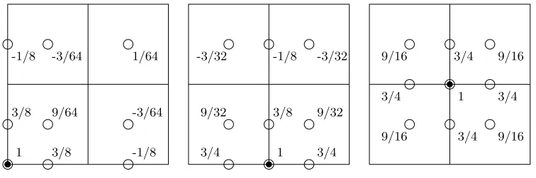
Since the geometrical configuration is more complicated for theQ2-square element, we only give in Figure 6

the non-zero coefficients in the refinement equation associated to three coarse basis functions. More precisely, on each picture, the coarse basis function represented by a black bullet is the linear combination of the finer basis functions represented by circles with the coefficients mentionned nearby. The other refinement equations can be readily obtained by symmetry.

-1/8

3/8 1

9/64

3/8 -3/64

1

3/8

3/4 9/32 1/64

-3/64 -1/8

9/32

3/4 -3/32 -1/8

-3/32 9/16 3/4 9/16

3/4 1

3/4

9/16 3/4 9/16

Figure 6. Q2-square refinement coefficients.

1.3.

Multilevel finite element approximation spaces

Let Ω be a bounded domain of Rd_{, d = 1,2 or 3. The purpose of this section is to give an automatic}

way to construct H1_{(Ω)-conformal multilevel finite element approximation spaces from an initial geometrically}

meshesT0,T1, . . . ,TJ fromT0 by applying uniformly and recursively the refinement pattern. Then, a multilevel

approximation space is obtained by selecting some basis functions associated to each meshTj, 06j6J in a way that guarantees linear independence of the selected basis functions.

1.3.1. Hierarchy of nested H1_{(Ω)-conformal approximation spaces. Parent-child relationship}

Let (K,b Σb,P ,b Tb) be a refinement pattern andj ∈J0, J−1K. In this subsection, we assume that a geometrically conformal mesh Tj = {Ke[j]; 1 6 e 6 Ne[j]} of Ω is given, that this mesh Tj is generated using the reference

element (K,b Σb,Pb), and then we explain how we can build the meshTj+1.

In the sequel, all mathematical objects associated to the meshTj will be marked with the signj as follows:

• Te[j] is the geometric mapping used to generateKe[j], i.e. Ke[j]=Te[j](Kb), • {a[1j], . . . ,a[j]

N_dof[j]}is the set of the Lagrange nodes of the meshTj, called level-[j] nodes, • Bj={ϕ[1j], . . . , ϕ

[j]

N_dof[j]} is the set of basis functions of the meshTj, called level-[j] basis functions, • Xj={v∈C0(Ω); ∀e∈J1, Ne[j]K, v_|K[j]

e ∈P

[j]

e }is the H1(Ω)-conformal approximation space associated

toTj.

Owing to Proposition 1.10, the following result holds:

Bj is a basis of the H1(Ω)-conformal approximation spaceXj.

Definition 1.15. We define the setTj+1 as follows: Tj+1=

n

K_ef[j+1]=T[j] e (Kb

[1]

f ); 16e6N [j]

e ,16f 6Nbe[1] o

.

Proposition 1.16. The setTj+1 is a geometrically conformal mesh ofΩgenerated by the reference elementKb.

Sketch of the proof. For the sake of simplicity, we only give here a sketch of the proof. It is straightforward to see thatTj+1 is a mesh of Ω. Hence, we only have to prove that it is geometrically conformal. LetK_ef[j+1] and K_e[j′+1]_f′ be two cells which have a non empty (d−1)-dimensional intersection, sayF =K

[j+1] ef ∩K

[j+1] e′_f′ . The

proof is based on different arguments depending on whether e = e′ _{or e 6= e}′_{. In the first case, we use the}

geometric conformity ofTb whereas in the second case the result is deduced from the geometrical conformity of

Tj and compatibility requirements 1.12.

The last point of the compatibility requirements 1.12 obviously ensures that a level-[j] node is also a level-[j+ 1] node. That is

∀k∈J1, N_dof[j]K, ∃ℓ∈J1, N_dof[j+1]K, a_k[j]=a[_ℓj+1]. (1)

We can now prove that our construction leads to embedded approximation spaces:

Proposition 1.17. It holds that Xj ⊂Xj+1.

Proof. Letv ∈Xj, e∈ {1, . . . , Ndof[j]} andf ∈ {1, . . . ,Nb [1]

e }. By definition, v_|K[j]

e ∈P

[j]

e . This is equivalent to

v◦Te[j]∈Pb. Using the compatibility requirements 1.12, we havev◦Te[j]_|Kb[1]

f ∈

b

P_f[1]. Hence, we getv◦Te[j]◦Tbf ∈Pb,

which exactly means thatv_|K[j+1]

ef

∈P_ef[j+1], and the claim is proved.

For the following result, we have to introduce relevant indexation of level-[j] and level-[j+1] nodes. Note that level-[j] and level-[j+ 1] nodes belonging to Ke[j] are, by definition, image of nodes ofΣ andb Σb[1] respectively

• I[j]_{(e, k) the index of the level-[j] node which is the image of b}

ak under the mappingTe[j]. That is

∀(e, k)∈J1, N[j]

e K×J1,NbK, a_I[j[]j]_(e,k)=T

[j] e (bak).

• I[j,1]_{(e, ℓ) the index of the level-[j+ 1] node which is the image of b}

a[1]_ℓ under the mappingTe[j]. That is

∀(e, ℓ)∈J1, N[j]

e K×J1,Nb[1]K, a [j+1]

I[j,1]_(e,ℓ)=T

[j] e (ba

[1] ℓ ).

Proposition 1.18(Refinement equation). The following relationship holds:

∀i∈J1, Ndof[j]K, ϕ

[j] i =

N_dof[j+1] X

t=1

β[_itj]ϕ[tj+1] (RE)

where the coefficientsβ_it[j] are given by: ∀(i, t)∈J1, Ndof[j]K×J1, N

[j+1]

dof K,

β[_itj] =

b

βkℓ if ∃(e, k, ℓ)∈J1, Ne[j]K×J1,NbK×J1,Nb[1]Ks.t. i=I[j](e, k)andt=I[j,1](e, ℓ),

0 otherwise.

Remark 1.19. Note that the coefficientsβbkℓ only depend on the refinement pattern. Hence, these coefficients

can be computed beforehand. They are in small number and therefore, requiring a low memory cost, they can be stored. Thus, the above refinement equations can be deduced without computation of any coefficient. In practice, coefficientsβ_it[j] are obtained thanks to a loop on level-[j] cells included in supp[ϕ[_ij]] by setting: for all

e∈J1, Ne[j]Ksuch thatKe[j]⊂supp[ϕi[j]], for all (k, ℓ)∈J1,NbK×J1,Nb[1]K,

β_I[j[j]]_(e,k)I[j,1]_(e,ℓ)=βbkℓ,

and other coefficients are zero. Remark that, such a loop may lead to consider several times the same pair of indices (I[j]_{(e, k), I}[j,1]_{(e, ℓ)) for distincte, k, ℓ. Proposition 1.18 ensures that corresponding coefficientsβb}

kℓ are

the same.

Proof of Proposition 1.18. Leti∈J1, Ndof[j]K. The basis functionϕ [j]

i belongs toXj. SinceXj ⊂Xj+1and Bj+1

is a basis ofXj+1, the existence of the coefficientsβ[itj] is straightforward.

Let (i, t)∈J1, Ndof[j]K×J1, N [j+1]

dof K. We have:

ϕ[_ij]=

N_Xdof[j+1]

t=1

β_it[j]ϕ[_tj+1]. (2)

• Case 1 : there exists (e, k, ℓ)∈J1, Ne[j]K×J1,NbK×J1,Nb[1]Ksuch thati=I[j](e, k) andt=I[j,1](e, ℓ).

The restriction of (2) toKe[j] yields:

b

ϕk◦

T[j] e

−1

=

b N[1] X

l=1

β[_iIj][j,1]_(e,l)ϕ

[j+1] I[j,1]_(e,l).

Owing to Proposition 1.14, we have:

b N[1] X

l=1 b

βklϕb[1]l ◦

T[j] e

−1

=

b N_X[1]

l=1

β[_iIj][j,1]_(e,l)ϕb

[1] l ◦

T[j] e

Evaluating this equality atTe[j](ab[1]_ℓ ), it follows that β_iI[j][j,1]_(e,ℓ)=βbkℓ. This is exactlyβ

[j] it =βbkℓ. • Case 2: ∀(e, k, ℓ)∈J1, Ne[j]K×J1,NbK×J1,Nb[1]K, i6=I[j](e, k) ort6=I[j,1](e, ℓ).

Let e ∈ J1, Ne[j]K and ℓ ∈ J1,Nb[1]K such that t = I[j,1](e, ℓ). We necessarily have, by assumption, ∀k∈J1,NbK, i6=I[j]_{(e, k). Hence, we get:}

0 =

N_dof[j+1] X

s=1

β_is[j]ϕ[sj+1]|Ke[j] =

b N_X[1]

v=1

β_iI[j][j,1]_(e,v)ϕb

[1]

v ◦(Te[j])−1.

Evaluating this equality atT[j]_(b

a[1]_ℓ ) yieldsβ[_iIj][j,1]_(e,ℓ)= 0.This is exactly,β

[j] it = 0.

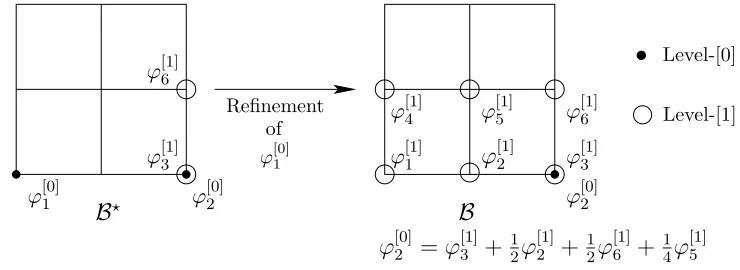
The refinement equation (RE) introduces a relationship between a level-[j] basis function and some level-[j+1] basis functions which are called its children.

Definition 1.20 (Parent-child relationship for basis functions). In the case whereβ_it[j]6= 0, we say that:

• the level-[j] basis function ϕ[_ij] is a parent of the level-[j+ 1] basis functionϕ[_tj+1],

• the level-[j+ 1] basis functionϕ[_tj+1] is a child of the level-[j] basis functionϕ[_ij].

For this reason, the refinement equation (RE) is also called the parent-child relationship. Along the same lines, we can define a parent-child relationship for cells.

Definition 1.21 (Parent-child relationship for cells). Lete∈J1, Ne[j]K.

• For allf ∈ {1, . . . ,Nbe[1]}, we say that the level-[j+ 1] cellK_ef[j+1] is a child cell of the level-[j] cellKe[j]. • Conversely, we say that the level-[j] cell Ke[j] is the parent cell of each level-[j+ 1] cell K_ef[j+1], for

f ∈ {1, . . . ,Nbe[1]}.

Remark 1.22. A cell has at most one parent cell whereas a basis function may have several parents. Never-theless, let us identify some basis functions which have only one parent.

Proposition 1.23(Private Child). Let (k, ℓ)∈J1, Ndof[j]K×J1, N

[j+1]

dof K such thata

[j] k =a

[j+1]

ℓ Then,

ϕ[_kj] is the unique parent of ϕ[_ℓj+1].

Proof. For 16i6N_dof[j], the parent-child relationship yields:

ϕ[_ij](a[_kj]) =

N_Xdof[j+1]

t=1

β_it[j]ϕ_t[j+1](a[_ℓj+1]).

This is exactly:

δik =β [j] iℓ.

Thus, the basis functionϕ[_ℓj+1] has a unique parent which is ϕ[_kj].

Summary 1.24. Let (K,b Σb,P ,b Tb) be a refinement pattern. Let T0 be a geometrically conformal mesh of Ω

generated using the reference element (K,b Σb,Pb). By applying uniformly the refinement pattern as described in this section, we are able to construct:

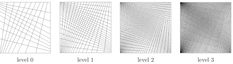
• a hierarchy of nested meshes,T0, T1, . . . , TJ (Figures 7, 8, 9),

• a hierarchy of nested H1_{(Ω)-conformal finite element approximation spacesX}

Mesh Basis Function Set Approximation Space

Level 0 T0 B0={ϕ[0]_k ;k= 1, . . . , Ndof[0]} X0 = span B0

Level 1 T1 B1={ϕ[1]k ;k= 1, . . . , N [1]

dof} X1 = span B1

..

. ... ... ... ...

Level J TJ BJ ={ϕ[kJ];k= 1, . . . , N [J]

dof} XJ = span BJ

Table 1. Conceptual hierarchy of nested conformal FE spaces.

level 0 level 1 level 2 level 3

Figure 7. Square-Q1. Nested meshesTj.

• basis function sets B0, B1, . . . ,BJ, spanning the above approximation spaces such that two consecutive

sets are linked by refinement equations,

Table 1 gives a summary of notations used in the sequel.

level 0 level 1 level 2 level 3

Figure 8. Tri/Quadr-angle-P1/Q1. Nested meshesTj.

level 0 level 1 level 2 level 3

Figure 9. Quadrangle-Q1. Nested meshesTj.

1.3.2. Multilevel basis and multilevel approximation spaces

We assume that a structure as presented in Summary 1.24 is given and we use the same notation (Table 1).

The aim of this subsection is to explain how we can select some basis functions in

J [

j=0

Bj in order to ensure the

linear independence of the selected family.

Proposition 1.25. Let B be a subset of SJ_j=0Bj. In the case where two nodes associated to distinct basis

functions of Bdo not have the same location, i.e.

 ∀(j, j

′_{)∈J0, JK}2_{, ∀(k, k}′_{)∈J1, N}[j]

dofK×J1, N

[j′]

dofK such thata

[j] k =a

[j′] k′ ,

(ϕ[_kj]∈ B, ϕ[_kj′′] ∈ B) =⇒(j=j′, k=k′), 

 (PLI)

thenB is linearly independent.

Remark 1.26. Note that (a[_kj]=a[j

′_]

k′ and j=j′) =⇒k=k′.

Proof. The property (PLI) implies that 

∀(j, j

′_{)∈J0, JK}2_{, ∀(k, k}′_{)∈J1, N}[j]

dofK×J1, N [j′]

dofK such thatj′> j,

(ϕ[_kj]∈ B, ϕ_k[j′′]∈ B) =⇒ϕ [j′] k′ (a

[j] k ) = 0,



 (3)

because, owing to (1), a[_kj] is also a level-[j′] node and, by (PLI), this node is certainly different from a[j

′_] k′

(otherwise j′_{=j ). Consider a linear combination of basis functionsϕbelonging toBsuch that} X

ϕ∈B

λϕϕ= 0, (4)

and assume thatE ={ϕ∈ B;λϕ6= 0}is not empty. We can then define

jm= min{j∈J0, JK;∃k∈J1, Ndof[j]Ksuch thatϕ [j] k ∈ E},

and select a km ∈ J1, N [jm]

dof K such that ϕ [jm]

km ∈ E. Let j ∈ J0, JK and k ∈ J1, N

[j]

dofK such that ϕ [j]

k ∈ E and

(j, k)6= (jm, km). Owing to (3), we haveϕ [j] k (a

[jm]

km ) = 0. Hence, evaluating the linear combination (4) ata

[jm]

km yieldsλ_ϕ[jm]

km = 0. This is a contradiction and the claim is proved.

Definition 1.27(Multilevel basis and multilevel approximation space). We call a multilevel level basis a subset

Bof

J [

j=0

Bjsatisfying the property (PLI). By Proposition 1.25, this set is actually independent. A space spanned

by a multilevel basis is called multilevel approximation space.

Remark 1.28. Let V = span B be a multilevel approximation space and u ∈ V. The coordinates of the expansion of u in the multilevel basis B are not necessarily the values of u at the nodes associated to the corresponding basis function, since two basis functions of different levels may have overlapping supports.

2.

Adaptation procedure and multigrid preconditioners

The adaptation consists in adding or removing some basis functions of a given multilevel basisB⋆ _{in order}

to produce a new multilevel basis B whose spatial resolution will be better suited to the problem. The main points are to ensure that the Un/Refinement algorithm will actually produce a linearly independent family of basis functions, and that no information is loss during the refinement process. Section 2.1 is devoted to the proofs of such properties. Then, in Section 2.2, we show how to also use the multilevel structure obtained by the adaptation algorithm in order to build a multigrid preconditioning algorithm which let us solve a multilevel linear system with a moderate computational cost.

2.1.

Adaptation

2.1.1. Refinement/Unrefinement procedures

Given a multilevel basisB, let us first introduce the notion ofB-refined basis functions.

Definition 2.1 (B-refined basis functions). Let B a multilevel basis. Let j ∈J0, JK and k ∈J1, Ndof[j]K. The

basis functionϕ[_kj] is said to be B-refined iff:

∃j′∈Jj+ 1, JK, ∃k′ ∈J1, N_dof[j′]K, such thatϕ_k[j′′]∈ B anda[_kj] =a[j

′_] k′ .

Moreover, if the above condition holds forj′_{=j+ 1 then we say that the basis function ϕ}[j]

k is B-refined only

once.

Remark 2.2. Owing to Property (PLI), notice that: • the indicesj′ _andk′ _{are necessarily unique.} • a B-refined basis function does not belong toB.

Remark also that, by Proposition 1.23, ifϕ[_kj] is only onceB-refined thenϕ_k[j] is the unique parent of ϕ[_kj′′].

Let us give the following lemma which will be useful in the following proofs.

Lemma 2.3. Letj∈J0, JKandj′ _{∈J0, J−1Ksuch thatj}′_{6j. Let(k, ℓ, ℓ}′_{)∈J1, N}[j]

dofK×J1, N

[j+1]

dof K×J1, N

[j′_]

dofK.

Ifa[_ℓj+1] =a[j

′_] ℓ′ andϕ

[j]

k is a parent ofϕ [j+1]

ℓ then the nodea

[j]

k is necessarily at the same position that the nodes

a[j

′_]

ℓ′ anda[_ℓj+1].

Proof. Since j′ _{6j, owing to (1) and a straightforward recurrence, there existst ∈J1, N}[j]

dofK such thata [j] t =

a_ℓ[j+1]. We can apply Proposition 1.23 which proves thatϕ[_tj] is the unique parent ofϕ_ℓ[j+1]. Hence,ϕ[_kj]=ϕ[_tj]

and then, k=t.

We can now describe the refinement and unrefinement procedure.

• Refinement: Let ϕ[_kj] be a basis function belonging to B⋆_.

Refining the given basis function ϕ[_kj] ∈ B⋆ _{consists in producing a new multilevel basisB by} – removing this basis functionϕ[_kj], and

– adding all its childrenϕ[_ℓj+1] which are not B⋆_-refined.

This can be written in a compact way as follows:

B=B⋆_\{ϕ[j]

k } ∪ {children ofϕ [j]

k not B⋆-refined}.

• Unrefinement: Letϕ[_kj] be an only onceB⋆_{-refined basis function without B}⋆_{-refined children.}

Unrefining the given basis function ϕ[_kj]6∈ B⋆ _{consists in producing a new multilevel basisB by} – adding this basis functionϕ[_kj], and

– removing those children ofϕ[_kj] which have no other B⋆_{-refined parent .}

This can be written in a compact way as follows:

B=B⋆_{\{children ofϕ}[j]

k without other B

⋆_{-refined parent} ∪ {ϕ}[j] k }.

Proof. As claimed in the above algorithm, we have to prove that refinement and unrefinement procedures produce actually a multilevel basis. That is to say thatBsatisfies the property (PLI). Indeed, letϕ[_kj],ϕ[j

′_] k′ two

basis functions belonging toB such thata[_kj]=a[j

′_]

k′ . We have to show thatj=j′.

• Refinement: Assume thatBis obtained fromB⋆_{by the refinement of a basis function belonging toB}⋆_,

sayϕ[j0] k0 ∈ B

⋆_{, so that we have}

B=B⋆_\{ϕ[j0]

k0 } ∪ {children ofϕ

[j0] k0 notB

⋆_-refined}.

– Ifϕ[_kj] andϕ[_kj′′]belong both toB⋆then, sinceB⋆satisfies the property (PLI), we readily findj=j′. – Otherwise, assume for instance thatϕ[_kj] does not belong toB⋆_{. By definition of B, ϕ}[j]

k is then a

child ofϕ[j0]

k0 which is notB

⋆_{-refined, sayϕ}[j0+1]

ℓ0 , i.e. k=ℓ0, j=j0+ 1. ∗ Ifϕ[_kj′′]∈ B⋆then, sinceϕ

[j0+1]

ℓ0 is notB

⋆_{-refined, we havej}

0+1>j′. Assume thatj0+1> j′.

Lemma 2.3 yields a[_kj₀0] =a[j

′_]

k′ . SinceB⋆ satisfies the property (PLI), we obtain j0=j′ and k0=k′, butϕ_k[j₀0] 6∈ Bandϕ[j

′_]

k′ ∈ B. This is a contradiction and we getj=j0+ 1 =j′. ∗ Otherwise, ϕ[_kj′′] is a child ofϕ

[j0] k0 , sayϕ

[j0+1] ℓ0′ , i.e. k

′ _=ℓ

0′ and j=j0+ 1. Hence, we have j=j′_.

• Unrefinement: Assume that Bis obtained fromB⋆ _{by the unrefinement of a only onceB}⋆_{-refined basis}

function, sayϕ[j0]

k0 , so that we have

B=B⋆_{\{children ofϕ}[j0]

k0 without otherB

⋆_{-refined parent} ∪ {ϕ}[j0] k0 }.

– Ifϕ[_kj] andϕ[_kj′′] belong toB⋆ then, sinceB⋆satisfies the property (PLI), we getj=j′.

– Otherwise, assume for instance that ϕ[_kj] does not belong to B⋆_{. By definition of B, we have}

ϕ[_kj] = ϕ[j0]

k0 , i.e. k = k0, j = j0. Arguing by contradiction, we assume that j

′ _{6= j. We have}

j′_6=j

0 and so,ϕ[j ′_]

k′ ∈ B⋆. However,ϕ [j0]

k0 is an only onceB

⋆_{-refined basis function, so there exists}

ℓ0∈J1, Ndof[j0]Ksuch thatϕ [j0+1] ℓ0 ∈ B

⋆_and

a[_ℓj₀0+1] =a[_kj₀0]. Owing to Proposition 1.23,a[_ℓj₀0+1] =a[_kj₀0] implies thatϕ[j0]

k0 is the unique parent ofϕ

[j0+1]

ℓ0 . Therefore, sinceϕ

[j0+1]

ℓ0 is a child ofϕ

[j0]

k0 without

otherB⋆_{-refined parent, we getϕ}[j0+1]

ℓ0 6∈ B. However, sinceB

⋆_{satisfies the property (P}

a[_ℓj₀0+1] =a[j

′_]

k′ , we havej′=j0+ 1 andk′ =ℓ0. Finally, we getϕ[j ′_]

k′ 6∈ B. This is a contradiction

and we obtainj=j′_.

Remark 2.5. This algorithm is consistent with Definition 2.1. Indeed, owing to Proposition 1.23,

• if B is obtained from B⋆ _{by the refinement of the basis function ϕ}[j]

k , then ϕ [j]

k is a B-refined basis

function in sense of Definition 2.1 ;

• ifB is obtained fromB⋆ _{by the unrefinement of the only onceB}⋆_{-refined basis functionϕ}[j]

k , thenϕ [j] k

is no longer aB-refined basis function in the sense of Definition 2.1.

ϕ

ϕ

B

of ϕ[0]1

ϕ

ϕ

B

ϕ

ϕ

ϕ

ϕ

ϕ

ϕ

Level-[0]

ϕ

ϕ

=

ϕ

+

ϕ

[1] 2

+

ϕ

[1] 6

+

ϕ

[1] 5

Figure 10. Refinement do not preserve the linear independence of multilevel set not satifying (PLI).

Remark 2.6. Refinement and unrefinement procedure described in Algorithm 2.4 do not preserve in general the linear independence of multilevel basis function set

J [

j=0 e

Bj (withBje ⊂Bj) which do not satisfy the property

(PLI). An example is given in Figure 10. The familyB⋆represented on the left hand-side is linearly independent

(but do no satisfy (PLI)) whereas the familyB, on the right hand-side, obtained fromB⋆ by refinement ofϕ[0]1 ,

is not a linear independent family.

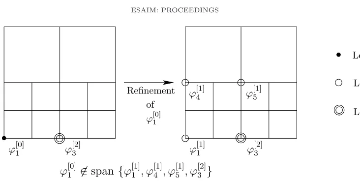
2.1.2. Conservation of information

A desirable property of a refinement procedure is that it does not involve a loss of information. It means that, ifB is obtained fromB⋆ _{by refinement of a basis function, then spanB}⋆_{⊂span B, i.e. the refined basis} Ballows for any function in the original basisB⋆ _{to be reproduced exactly. However, the refinement procedure}

described in Algorithm 2.4 is not lossless. An example is given in Figure 11. Nevertheless, we can prove the following results.

Proposition 2.7. Let B be a multilevel basis satisfying the following property:

A child of a B-refined basis function either belongs toB or is itselfB-refined. (PLO)

Then, all B-refined basis functions belong tospanB.

Proof. By a recurrence on the leveljof basis functions, we prove the following statement (Hj) for allj∈J0, JK:

All level-[j]B-refined basis functions belong to spanB. (Hj)

Level-[2] Level-[0]

ϕ

ϕ

ϕ

ϕ

ϕ

Refinement

ϕ[0]₁ of

Level-[1]

ϕ

ϕ

6∈

span

{

ϕ

, ϕ

, ϕ

, ϕ

}

Figure 11. Refinement of multilevel basis is not lossless.

Letj∈J0, J−1K. Assume that the statement (Hj+1) holds and letϕ[_kj]be a level-[j]B-refined basis function.

Owing to Proposition 1.18, we have

ϕ[_kj]= X

ℓ|ϕ[_ℓj+1]is a child ofϕ[_kj]

β_kℓ[j]ϕ[_ℓj+1].

Moreover, property (PLO) implies that all basis functions ϕ[_ℓj+1] involving in the above sum are either inB or B-refined. In the last case, the recurrence assumption (Hj+1) yieldsϕ[_ℓj+1]∈spanB. Hence,ϕ[_kj] ∈spanBand

the recurrence is established.

Theorem 2.8. Let B be a multilevel basis satisfying property (PLO)and obtained from the multilevel basis B⋆

by the refinement procedure (Algorithm 2.4), then

spanB⋆_⊂spanB.

Proof. Assume thatBis obtained fromB⋆ _{by the refinement of the basis functionϕ}[j0] k0 ∈ B

⋆_{. Letϕ}[j] k ∈ B⋆.

• Ifϕ[_kj]6=ϕ[j0] k0 thenϕ

[j] k ∈ B, • elseϕ[_kj]=ϕ[j0]

k0 which isB-refined. Proposition 2.7 ensure that ϕ

[j]

k ∈spanB.

Then spanB⋆_⊂spanB.

Moreover, the refinement and unrefinement procedures preserve the property (PLO). Let us begin with the

following lemma.

Lemma 2.9. Let B⋆ _{and B be two multilevel basis. Let ϕ}[j⋆]

k⋆ be a B⋆-refined basis function and ϕ

[j] k be a B-refined basis function.

1) If B is obtained fromB⋆ _{by the refinement of a basis functionϕ}[j0] k0 ∈ B

⋆ _then

(i) ϕ[_kj⋆⋆] is also B-refined,

(ii) ϕ[_kj] is eitherB⋆_{-refined or equal toϕ}[j0] k0 .

2) If B is obtained fromB⋆ _{by the unrefinement of an only onceB}⋆_{-refined basis functionϕ}[j0] k0 then

(i) ϕ[_kj⋆⋆] is either B-refined or is equal to ϕ

[j0] k0 ,

(iii) Moreover, if we assume thatϕ[_kj⋆⋆] is only onceB⋆-refined thenϕ

[j⋆_]

k⋆ is either also only onceB-refined

or is equal toϕ[j0] k0 .

Proof. Sinceϕ[_kj⋆⋆]isB⋆-refined, there existsj⋆′> j⋆andk⋆′ ∈J1, N

[j⋆′_]

dof Ksuch thatϕ [j⋆′_]

k⋆′ ∈ B⋆anda[j ⋆_]

k⋆ =a

[j⋆′_] k⋆′ .

Along the same lines, since ϕ[_kj] is B-refined, there existsj′ _{> j and k}′ _{∈ J1, N}[j′]

dofK such that ϕ [j′]

k′ ∈ B and

a[_kj] =a[j

′_] k′ .

1) Refinement ofϕ[j0] k0 .

(i) If ϕ[_kj⋆⋆′′]∈ B thenϕ [j⋆]

k⋆ isB-refined; elseϕ

[j⋆′] k⋆′ =ϕ

[j0]

k0 and sinceϕ

[j0]

k0 isB-refined, a fortioriϕ

[j⋆] k⋆ is

B-refined.

(ii) If ϕ[_kj′′] ∈ B⋆ thenϕ [j]

k isB⋆-refined and the claim is proved. Otherwise,ϕ [j′]

k′ is a child ofϕ [j0] k0 , say

ϕ[j0+1] ℓ0 , i.e. j

′_=j

0+ 1,k′=ℓ0. We havea[_kj] =a[_ℓj₀0+1] and j0+ 1> j, then owing to Lemma 2.3,

a[_kj]=a[_kj₀0]. Ifj0=j thenϕ[_kj]=ϕ[_kj₀0]; elsej0> j, sinceϕ_k[j₀0]∈ B⋆,ϕ[_kj] isB⋆-refined.

2) Unrefinement ofϕ[j0] k0 .

(i) Ifϕ[_kj⋆⋆′′] ∈ Bthenϕ [j⋆]

k⋆ isB-refined and the claim is proved. Otherwise,ϕ

[j⋆′]

k⋆′ is a child ofϕ [j0] k0 , say

ϕ[j0+1] ℓ0 , i.e. j

⋆′_=j

0+ 1,k⋆′ =ℓ0. We have a[j ⋆_]

k⋆ =a

[j0+1]

ℓ0 and j0+ 1> j

⋆_{, then owing to Lemma}

2.3,a[j ⋆_]

k⋆ =a[_kj₀0]. Ifj0=j⋆ thenϕ[j

⋆_]

k⋆ =ϕ

[j0]

k0 ; elsej0> j

⋆_{, sinceϕ}[j0] k0 ∈ B,ϕ

[j⋆_]

k⋆ is B-refined. (ii) If ϕ[_kj′′] ∈ B⋆ thenϕ

[j]

k isB⋆-refined; else ϕ [j′] k′ =ϕ

[j0]

k0 and sinceϕ

[j0] k0 is B

⋆_{-refined, a fortioriϕ}[j] k is B⋆_-refined.

(iii) Here, we assume that j⋆′ _=j⋆_{+ 1. If ϕ}[j⋆′_]

k⋆′ ∈ B then ϕ [j⋆_]

k⋆ is only once B-refined and the claim is proved. Otherwise, ϕ[_kj⋆⋆′′] is a child of ϕ

[j0]

k0 . However,owing to Remark 2.2,ϕ

[j⋆_]

k⋆ is the unique parent ofϕ[_kj⋆⋆′′]. Hence, we getϕ

[j⋆_]

k⋆ =ϕ

[j0] k0 .

Proposition 2.10. The refinement and unrefinement procedures of multilevel basis (in the sense of Algorithm 2.4) preserves the property (PLO).

Proof. Assume that the multilevel basisB⋆ _{satisfies the property (P}

LO). Letϕ[_kj] be aB-refined basis function

andϕ[_ℓj+1] be a child ofϕ_k[j]. We have to show thatϕ[_ℓj+1] either belong toBor isB-refined.

• Refinement: Assume that the multilevel basisBis obtained fromB⋆_{by the refinement of a basis function}

ϕ[j0] k0 ∈ B

⋆_{. By Lemma 2.9 property 1) (ii),ϕ}[j]

k is either B⋆-refined or equal toϕ [j0]

k0 . Consider the two

cases:

– Ifϕ[_kj] isB⋆_{-refined. SinceB}⋆_{satisfies the property (P}

LO), only the two following cases are possible: ∗ ϕ[_ℓj+1]isB⋆_{-refined. Owing to Lemma 2.9 property 1)(i), this implies thatϕ}[j+1]

ℓ isB-refined. ∗ ϕ[_ℓj+1]∈ B⋆_{. And then,ϕ}[j+1]

ℓ ∈ B orϕ [j+1]

ℓ =ϕ

[j0]

k0 which isB-refined. – Ifϕ[_kj] =ϕ[j0]

k0 , all its children are either inBor areB

⋆_{-refined. Owing to Lemma 2.9 property 1)(i),}

they are either inBor B-refined.

• Unrefinement: Assume that B is obtained from B⋆ _{by the unrefinement of an only once refined basis}

functionϕ[j0] k0 of B

⋆_{. By Lemma 2.9 property 2) (ii),ϕ}[j]

k is B⋆-refined. SinceB⋆ satisfies the property

(PLO), only the two following cases are possible:

– ϕ[_ℓj+1] is B⋆_{-refined. Owing to Lemma 2.9 property 2)(i), this implies that ϕ}[j+1]

ℓ is B-refined or

ϕ[_ℓj+1] =ϕ[j0] k0 ∈ B.

– ϕ[_ℓj+1] ∈ B⋆_{. And then, we haveϕ}[j+1]

ℓ ∈ B or ϕ [j+1]

ℓ is a child of ϕ

[j0]

k0 with no other B

⋆_-refined

haveϕ[_kj] = ϕ[j0]

k0 . However, ϕ

[j0]

k0 is not a B-refined function. This is a contradiction and we get

ϕ[_ℓj+1] ∈ B.

Remark 2.11. Note that the properties (PLI) or (PLO) are not so restrictive since they are preserved by

Un/Refinement procedures and since it is straightforward to see that they are satisfied by the coarse basis B0

which is used, in practice, for starting the adaptation algorithm. 2.1.3. Adaptation procedure

Proposition 2.12. Let B⋆ _{be a multilevel basis.}

1) Let E⋆ _{⊂ B}⋆_{. It is possible to refine successively all basis functions belonging to E}⋆_{, hence producing a}

multilevel basisB which is independent of the order in which the basis functions were refined. We say thatB is obtained fromB⋆ _{by the refinement of the set of basis functionsE}⋆_.

2) Let F⋆ _{be a set of only once B}⋆_{-refined basis functions which have noB}⋆_{-refined child. It is possible to}

unrefine successively all basis functions belonging to F⋆_{, hence producing a multilevel basisB which is}

independent of the order in which the basis functions were unrefined.

We say thatB is obtained fromB⋆ _{by the unrefinement of the set of basis functions F}⋆_.

Proof. In the two cases, we first have to prove that successive (un)refinements are possible and then that the obtained multilevel basisBis independent of the order in which the basis functions are (un)refined.

1) – Letϕ∈ E⋆_{. The setE}⋆_{\{ϕ} is included in the multilevel basis produced by the refinement ofϕ}

since, in this procedure, onlyϕis removed fromB⋆_{. Hence, all basis functions inE}⋆_{\{ϕ} can be}

then refined.

– It is sufficient to prove thatBis independent of the order in which the basis functions are refined in the case where #E⋆ _{= 2, sayE}⋆ _{={ϕ, ψ}. Denote byB the multilevel basis obtained by the}

refinement ofϕinB⋆_{and then byBthe multilevel basis obtained by the refinement ofψinB. By}

definition, we have

B=B⋆_{\{ϕ} ∪ {children ofϕnotB}⋆_{-refined} (5)}

and

B=B\{ψ} ∪ {children ofψnotB-refined} (6)

Applying Lemma 2.9 property 1) (i) and (ii), we get

{B-refined basis functions}={B⋆_{-refined basis functions} ∪ {ϕ} (7)}

Hence, combining (6) and (7), we obtain

B=B\{ψ} ∪ {children ofψ notB⋆_{-refined and different fromϕ} (8)}

Combining (5) and (8), we get

B= B⋆_{∪ {children ofϕandψwhich are notB}⋆_{-refined}\{ϕ, ψ}.}

This expression shows thatB do not depend of the order in which the basis functionsϕandψ were refined.

2) – Letϕ∈ F⋆_{. Denote byBthe multilevel basis obtained by the unrefinement ofϕin B}⋆_{. We have}

to prove that all basis functions ofF⋆_{\{ϕ} can be unrefined in B,i.e. that any basis function of} F⋆_{\{ϕ}is only onceB-refined and has noB-refined children. Letψ∈ F}⋆_{\{ϕ}. Owing to Lemma}

– It is sufficient to prove thatBis independent of the order in which the basis functions are unrefined in the case where #F⋆_{= 2, say F}⋆_{={ϕ, ψ}. Denote byBthe multilevel basis obtained fromB}⋆

by the unrefinement ofϕand then byBthe multilevel basis obtained fromBby the unrefinement ofψ. By definition, we have

B=B⋆_{\{children ofϕwhich have no otherB}⋆_{-refined parent} ∪ {ϕ} (9)}

and

B=B\{children ofψ which have no otherB-refined parent} ∪ {ψ} (10)

Applying Lemma 2.9 property 2) (i) and (ii), we get

{B⋆_{-refined basis functions}={B-refined basis functions} ∪ {ϕ} (11)}

Hence, combining (10) and (11), we obtain

B=B\{children ofψwhich have noB⋆_{-refined parent except possiblyϕ} ∪ {ψ} (12)}

Combining (9) and (12), we get

B=B⋆_{\{children ofϕandψwhich have noB}⋆_{-refined parents except possiblyϕandψ} ∪ {ϕ, ψ}.}

This expression shows thatBdo not depend of the order in which the basis functionsϕandψwere refined.

With this definition at hand, we can give the refinement algorithm.

Algorithm 2.13 (Adaptation procedure). Let B⋆ _{a multilevel basis. Assume that, thanks to a refinement}

criterion, we are given the set E⋆_{⊂ B}⋆ _{of basis functions to refine and the setF}⋆ _{of only onceB}⋆_{-refined basis}

functions (withoutB⋆_{-refined children) to unrefine. The adaptation procedure consists in the two following steps:}

1) Refine the setE⋆_{, thus producing a new multilevel basis B.}

2) Unrefine the set of basis functions of F⋆ _{which are still only once B-refined basis functions without} B-refined children.

2.1.4. One-level-difference rule

In practice, the following criterion is used to ensure the common rule of “one-level-difference refinement” [15].

Criterion 2.14 (One-level-difference refinement rule). Let B⋆ _{a multilevel basis. A basis function of B}⋆ _may

be refined only if all its parents areB⋆_-refined.

Typically, this criterion is used to avoid an important difference of refinement level between “neighboring” basis functions. An example of refinement sequence forbidden by this criterion is given in Figure 12.

This criterion can be taken into account by adding a recursive step in the refinement procedure: to refine a basis function, we first refine all its parents which are notB⋆_{-refined and then we refine the basis function itself.}

This is illustrated, for instance, by the spreading of the level-[1] refined area between the first two pictures in Figure 17.

2.2.

Multigrid preconditioner

In this section, we assume that we have the following genuine variational problem to solve: Findu∈ Vhsuch that

Level-[0]

Level-[2]

Figure 12. Refinement sequence forbidden by the One-level-difference rule.

where Vh = spanB is a multilevel approximation space, a: H1_(Ω)×H1_{(Ω) →Ris a bilinear continuous and}

coercive form and b: H1_{(Ω)→Ris a linear continuous form. We denote byA}

J the stiffness matrix associated

to this problem, that is

AJ = [a(ϕ, ψ)]ϕ,ψ∈B.

The multilevel spaceVhis built to achieve a given level of accuracy without increasing too much the number

of degrees of freedom in the discrete problem. In fact, we are going to describe how to naturally take advantage of the multilevel structure of the approximation space in order to build a sequence of nested multilevel grids finally leading to a multigrid preconditioner.

2.2.1. Coarsening

From a given “fine” multilevel basisBF, the following algorithm is used to construct a “coarser” multilevel basisBC.

Algorithm 2.15 (Coarsening). Let BF a multilevel basis. Let jM = max{j∈J0, JK;BF∩Bj6=∅} be the

highest refinement level inBF. A “coarser” multilevel basisBC, denoted byBC= coarsen(BF), is obtained from

BF by unrefinement (Algorithm 2.4) of the set of BF-refined basis functions of level[jM−1].

The following proposition gives an equivalent formulation of the above algorithm.

Proposition 2.16. Assume thatBF is a multilevel basis satisfying the following property:

Any level-[j] basis function,j>1, which either belongs to B or isB-refined, has at least one

B-refined parent. (PHI)

Let jM = max{j∈J0, JK;BF∩Bj6=∅}. The multilevel basisBC= coarsen(BF)defined in Algorithm 2.15 can

be obtained by the following equivalent algorithm:

• remove all level-[jM] basis functions ofBF,

• add all BF-refined basis functions of level [jM −1].

Proof. Note first that any step in Algorithm 2.15 consists in an unrefinement of a level-[jM−1] basis function,

this implies that added basis functions are certainly on level-[jM −1] and that removed basis functions are

certainly on level-[jM]. Hence, the set of added and removed basis functions are disjoint. In Algorithm 2.15,

a basis function which is removed (or added) by an unrefinement procedure can not be added (or respectively removed) by an other unrefinement procedure. Furthermore, remark that by definition ofjM, there is noBF

-refined function on level-[jM]. Hence, since they have noBF-refined children, allBF-refined basis functions can

actually be unrefined. Unrefinement of a basis functions involved that it is added and then the set of added basis functions in Algorithm 2.15 is exactly the set of BF-refined basis functions. It remains to show that all

level-[jM] basis functions ofBF are removed. Arguing by contradiction, assume that a level-[jM] basis function

belongs to coarsen(BF). Since unrefinement preserves the property (PHI) (Proposition 2.17), this basis function

has at least one coarsen(BF)-refined parent. Owing to Lemma 2.9 property 2) (ii), this is also aBF- refined

The property (PHI) ensures the desirable fact that all level-[jM] basis functions ofBF are removed. This

additional property is not so restrictive since it is preserved by the refinement and unrefinement procedures.

Proposition 2.17. The refinement and unrefinement procedures described in Algorithm 2.4 preserve the prop-erty (PHI).

Proof. Assume thatB⋆ _{is a multilevel basis satisfying the property (P}

HI) and letj∈J1, JK. • Consider first a basis functionϕ[_kj] which belongs toB.

– Refinement: Assume that the multilevel basisB is obtained fromB⋆ _{by the refinement of a basis}

functionϕ[j0] k0 ∈ B

⋆_.

∗ Case 1: ϕ[_kj] ∈ B⋆_{. Since B}⋆ _{satisfies the property (P}

HI), ϕ[_kj] has at least one B⋆-refined

parent. Owing Lemma 2.9 property 1), this parent isB-refined.

∗ Case 2: ϕ[_kj] is a child ofϕ[j0] k0 andϕ

[j0]

k0 isB-refined.

– Unrefinement: Assume that B is obtained from B⋆ _{by the unrefinement of an only once refined}

basis functionϕ[j0] k0 ofB

⋆_.

∗ Case 1: ϕ[_kj]∈ B⋆_{\{children ofϕ}[j]

k without otherB⋆-refined parent}.

SinceB⋆ _{satisfies the property (P}

HI),ϕ[_kj] has at least oneB⋆-refined parent. Owing Lemma

2.9 property 2), either this parent isB-refined or this isϕ[j0] k0 .

In the first case, the proof is finished, in the second caseϕ[_kj] is a child ofϕ[j0]

k0 which belongs

to B⋆_{\{children ofϕ}[j]

k without otherB⋆-refined parent}. Therefore, ϕ [j]

k has an other B⋆

-refined parent. This parent is thenB-refined because it is notϕ[j0] k0 . ∗ Case 2: ϕ[_kj] =ϕ[j0]

k0 , ϕ

[j0] k0 is B

⋆_{-refined. Since B}⋆ _{satisfies the property (P}

HI), ϕ[_kj₀0] has at

least oneB⋆ _{refined parent. Owing Lemma 2.9 property 2), this parent isB-refined because}

it can not beϕ[j0] k0 .

• Consider now a basis functionϕ[_kj] which isB-refined.

– Refinement: Assume that the multilevel basisB is obtained fromB⋆ _{by the refinement of a basis}

functionϕ[j0] k0 ∈ B

⋆_{. By Lemma 2.9 property 1) (ii),ϕ}[j]

k is eitherB⋆-refined or equal toϕ [j0] k0 ∈ B

⋆_.

Since B⋆ _{satisfies the property (P}

HI), in the two cases, ϕ[_kj] has at least one B⋆-refined parent.

Owing to Lemma 2.9 property 1)(i), this parent is alsoB-refined.

– Unrefinement: Assume thatBis obtained fromB⋆_{by the unrefinement of an only once refined basis}

functionϕ[j0] k0 ofB

⋆_withoutB⋆_{-refined children. By Lemma 2.9 property 2) (ii),ϕ}[j]

k isB⋆-refined.

Since B⋆ _{satisfies the property (P}

HI), ϕ[_kj] has at least one B⋆-refined parent. Owing to Lemma

2.9 property 2) (i), either this parent is B-refined or is equal toϕ[j0]

k0 . The last case is impossible

becauseϕ[j0]

k0 has noB

⋆_{-refined children.}

The last main property of the coarsening procedure, is that it produced nested vector spaces.

Proposition 2.18. Let BF be a multilevel basis satisfying the property (PLO) and BC = coarsen(BF). The

following embedding holds:

span BC⊂spanBF.

Proof. Let ϕ∈ BC. If ϕ 6∈ BF then ϕ has been unrefined and so this is a BF-refined basis function of level

[jM −1]. Owing Proposition 2.7,ϕ∈span BF.

• either ϕ∈ BF

• or all the children of ϕbelong toBF and then, the refinement equation yields an expression of ϕas a linear combination of elements inBF.

Remark 2.20. Note that properties (PLO) and (PHI) used in this section are not so restrictive since they are

preserved by Un/Refinement procedures and since it is straightforward to see that they are satisfied by the coarse basis B0which is used, in practice, to start the adaptation algorithm. (see also Remark 2.11)

2.2.2. Multigrid framework

We recursively define a sequence{V0, . . . , VJ}of nested spaces built uponVhas follows: • we first takeBJ =B andVJ = spanBJ=Vh,

• then, fork=J, . . . ,1, we define a coarser multilevel basisBk−1from Bk by:

Bk−1= coarsen(Bk),

and the corresponding multilevel approximation space:

Vk−1= spanBk−1.

Owing to Proposition 2.18, we have:

V0⊂V1⊂ · · · ⊂VJ.

Note that the auxiliary sequenceV0 ⊂ · · · ⊂VJ introduced here usually do not reflect the dynamic refinement

process, although a such sequence can always be a posteriori deduced from any multilevel approximation space

VJ. An example with four refinement level is given in Figure 13.

V

Level-[1] basis functions Level-[3] basis functions Level-[2] basis functions Level-[0] basis functions

V

V

V

Figure 13. Example of coarsening : fromV3 toV0.

We do not need to know explicitly any information about the spaces Vk, except the intergrids operators.

Owing to Remark 2.19, it is staightforward to construct the matrix representation, denoted by Ik

k−1, of the

natural embedding from Vk−1 to Vk in the basisBk−1 and Bk. Then, intergrids operators are defined in the

following way, for allk∈J0, JK:

Ik =IJ−J 1IJ−J−21· · ·I k+1 k

We can also define approximate operators on each spaceVk, for allk∈J0, JKby:

Ak=IktAJIk

At last, in the sequel, we used Jacobi and Gauss-Seidel smoothers defined for allk∈J0, JKas follows:

• Jacobi: Sk=Dk whereDk is the diagonal part ofAk.

2.2.3. Multigrid Algorithm

We used the two following multigrid preconditioners:

• Additive version [8]:

Pa= J X

k=0 IkSkIkt

whereSk,k∈J0, JK, is the Jacobi smoother.

• Multiplicative version [12]: This correspond to the classical V-cycle. In this sectionSk is the

Gauss-Seidel smoother. We define recursively, for all k ∈J0, JK, the linear operator M Gk : R#Bk →R#Bk.

We first setM G0=A−01 and for allk∈J1, JK, we defineM Gk(fk),fk ∈R#Bk by the following steps:

(0) vk֋0 Initialisation

(1) vk֋vk+Sk(fk−Akvk), Pre-smoothing step

(2) vk֋vk+Ik−1M Gk−1(Ik−t 1(fk−Akvk)), Coarse Grid Correction

(3) vk֋vk+Sk(fk−Akvk), Post-smoothing step

SetM Gk(fk) =vk.

The multiplicative preconditioner is then

Pm=M GJ.

2.3.

Validation on a stationnary model problem

We first validate the local refinement method and the multigrid preconditioner on the following stationnary model problem.

The practical implementation has been performed using the software object-oriented component library PELICANS [19], developed at the “Institut de Radioprotection et de Sˆuret´e Nucl´eaire (IRSN)” and distributed under the CeCILL-C license agreement (an adaptation of LGPL to the French law).

2.3.1. Continuous model problem

Let Ω = [0,1]d_{. Consider the Laplace problem with homogeneous Dirichlet boundary conditions:}

−∆u = f in Ω,

u = 0 on∂Ω. (13)

The source term f is chosen so that the exact solution uis:

∀x∈Rd, u(x) =Hε

R− |x−xC|,

whereR∈R,ε∈R∗

+,xC∈Rd are parameters and Hε:R−→Ris defined by

∀x∈R, Hε(x) =         

0 ifx <−ε,

1 2

1 + x

ε +

1

πsin

πx ε

if|x|6ε,

1 ifx > ε.

The function Hε is represented in Figure 14 and the interpretation of parameters R, ε, xC is explained in

Figure 15 which represents the exact solutionuwhend= 1. For numerical simulations given in the sequel, we have set: