A New Nonparametric Regression for Longitudinal Data
Hamed Tabesh1 *Azadeh Saki1 Samira Mardaniyan2
1-Ph.D of Biostatistics, Department of Biostatistics and Epidemiology, School of Health, Ahvaz Jundishapur University of Medical Sciences
2-MSc. Student of Biostatistics, Department of Biostatistics and Epidemiology, School of Health, Ahvaz Jundishapur University of Medical Sciences
Original Article
Abstract
Background and purpose: In many area of medical research, a relation analysis between one response variable and some explanatory variables is desirable. Regression is the most common tool in this situation. If we have some assumptions for such normality for response variable, we could use it. In this paper we propose a nonparametric regression that does not have normality assumption for response variable and we focus on longitudinal data.
Materials and Methods: Consider nonparametric estimation in a varying coefficient model with
repeated measurements (Yij,X ij,tij), for i=1, …, n and j =1 ,… , ni where Xij=(X ijo,...,X ijk)T and
(Yij,X ij,tij) denote the jth outcome , covariate and time design points, respectively , of the ith subject.
The model considered here isYijYTij(tij)i(tij), where(t)(0(t),...,k(t))T,for k0, are
smooth nonparametric functions of interest and i(t)is a zero-mean stochastic process. The
measurements are assumed to be independent for different subjects but can be correlated at different time points within each subject. For evaluating this model, we use data of a cohort of 289 healthy infants born in Shiraz in 2007. The proposed nonparametric regression was fitted to them for obtaining effect rates of mother weight, mother arm circumference and maternal age at delivery time and maternal age at first menarche on boy’s arm circumference.
Results: proposed nonparametric regression showed the varied effect of each independent variable over the time but other models achieved constant effect over the time that is in controversy with the inherent property of these natural phenomena.
Conclusion: This study shows that this model and the spline nonparametric estimator could be useful in different areas of medical and health studies.
[Tabesh H. *Saki A. Mardaniyan S. A New Nonparametric Regression for Longitudinal Data. IJHS 2013;1(3):58-70]http://jhs.mazums.ac.ir
Key words: Cohort Studies, Longitudinal Data, Nonparametric Regression, Spline Smoothing.
IJHS 2013; 1(3): 59
1.
Introduction
With the increasing and developing of long-term cohort studies and clinical trial in the last three decades, importance of assessing the existing relationship that may be time-dependent will be appeared(1). For example, determination of short-term and long-term effects of zidovudine on CD4 cells (Repeated examination has been used in control and treatment groups in people who suffer from HIV) required to making statistical cost-benefit decision which whether the study should be continued or stopped(2). As another example, Modeling of the time effects to quantitative variables in children's anthropometric dimensions measurements could lead to a class of information about the effects of some factors on growth of children , also it could determine the effects of clinical interventions(3-4).So we can expect further progresses in the field of medical and biological studies to be done in line with cohort dataset. Although there are some statistical tools for analysis of these data but each of them have a limitations(5-6). For example, generalized additive semi-parametric models can be fitted to correlated data of cohorts with using existing software. Although such models can obtained consistent estimates for 0(t) and 0(t)
when
Y i
t X i t
0(t)0(t)X i
t (7).But deselect of correct model for 0(t) and ( ) 0 t
may lead to bias(2). Therefore, it seems to be required a nonparametric method for modeling 0(t)and0(t). Regarding to importance of
longitudinal studies and the ability of nonparametric methods for analysis of such data, analysis of longitudinal data seems interesting by using nonparametric regression models (8-10). In many longitudinal studies, repeated measurements are done for response variable at different and irregular time points. Suppose in a longitudinal study y(t) is the actual amount of the desired outcome and x (t) is a covariate vector Rk+1 - observed value at time t (k0). Also consider we have n subjects, for ith person
n
i≥ 1
carried out the repeated measures over time from
Y(t),X(t),t
.The jth observation from
Y(t),X(t),t
for ith subject is specified by
Yij,Xij,tij
for i1,...,nand j1,...,ni where1
k ij R
X is determined by the T
ijk ij
ij X X
X ( ,..., )
column vector. In the classical linear models framework, methods and theory of regression have been used for repeated observations in several studies(7). Methods such as weighted least squares , maximum likelihood ratio , limited maximum likelihood ratio or generalized linear models which used the quasi-likelihood method ,they are all examples of parametric methods that may be encountered the following problems when we used them:
1. Inaccuracy or inadequacy of model assumptions,
2.Inherent mistakes in the choice of models for data analysis. Due to these two reasons, using non-parametric methods are discussed(11).
IJHS 2013; 1(3): 60
Since easily understanding of regression methods many researchers are wishing to analyze their data by using regression methods, but the fundamental assumption in the regression methods is normality distribution of response variable. If the variable is not normal or does not hold the other assumptions of parametric regression model, with slight loss of efficiency and accuracy, nonparametric method could be used in order to obtain a model such as Yij Xij(tij)i(tij).
However, most researchers that have been done so far, have considered constant coefficients for predictor variables that makes a distance between fitted values and actual values of response variable. But where the coefficients were considered as functions of time, stochastic processes were used, which were required very long computational steps(12,13). In the present study, we try to find a solution to get the time varying coefficients in regression model which requires no complex calculation and its interpretation is easily possible.
2. Materials and Methods
In section 2-1 exposing with real longitudinal data showed and later after introducing proposed nonparametric regression, the application of this new method to the real data of section 2-1 is given.
2.1. Sampling and Participants
A cohort of 287 neonates (139 girls and 148 boys) were selected randomly among those born during July 10,2007 to September 10,2007 in Shiraz and visited by healthcare centers’ nurses during their first month of life. The healthcare were selected using cluster sampling scheme, with each healthcare center considered a cluster and the proportion of participants from each cluster being proportional to size of that healthcare center. The selected subjects were healthy singleton neonates without any medical complications whose mother residence of Shiraz. They were visited at healthcare centers at target ages 2,4,6 months and their arm circumference were measured in millimeters by nurses. A questionnaire completed at the time of recruitments to the study by the nurses in healthcare centers, included maternal and neonatal demographics and background data ( infant’s gender, birth weight, mother’s weight, mother’s age at delivery time and mother’s age at first menarche) also mother’s arm circumference were measured in millimeters(14-15).
2.2. Statistical Modeling
For modeling the boys’ arm circumference by mother’s weight, mother’s arm circumference, maternal age at delivery time and maternal age at menarche parametric or non-parametric regression methods can be used. In this study, a new method based on nonparametric proposed. In order to evaluate new method, results of the new model on the above data with output of the linear regression (parametric) and locally weighted regression (parametric) were compared.
2.2.1. Proposed nonparametric regression
Consider multiple regressions model in matrix by Y X that X can be a matrix of k
vectors. Whereas k independent random variables are predictor variables and i observation for each of them then the matrix X as follows.
IJHS 2013; 1(3): 61
Since
X
Y so
X
Y , as Yˆ Y thus Yˆ X (1)
Equation (1) is a matrix form e.g. Yˆ, X and are matrices. Whereas relationship between
a dependent variable and k independent variables are desired and i cases are contributed then aforementioned matrices shall be as follows:
1 1 Y i Y i Y k i X X X X X X X X ik ... i2 Xi1 2k ... 22 X21 1k ... 12 11 1 ˆ k ˆ 2 ˆ 1 k (2)
We can multiply both sides of equation (1) by 𝑋𝑇 from right-hand sides then we will have
𝑋𝑇𝑌 = 𝑋𝑇𝑋𝛽 𝑋𝑇𝑌 = (𝑋𝑇𝑋)𝛽 (3)
It is clear that 𝑋𝑇𝑋 is a square matrix. If this matrix can be inverted, that is certainly true
according to the enormous volume of information in growth data, and then we can multiply both sides of equation (3) in the inverse matrix (𝑋𝑇𝑋)
thus: (𝑋𝑇𝑋)−1𝑋𝑇𝑌 = (𝑋𝑇𝑋)−1(𝑋𝑇𝑋)𝛽 (𝑋𝑇𝑋) is invertible matrix so will give the identical matrix
e.g. (𝑋𝑇𝑋)−1𝑋𝑇𝑌 = 𝐼𝛽
Simply it can be shown that (𝑋𝑇𝑋)−1𝑋𝑇𝑌 = 𝛽 , Where 𝛽 is the desired coefficient matrix. By
obtaining the coefficient matrix for each considered model we should have an estimate of the response variable. Therefore, we estimate the fitted values for each model by locally weighted regression (loess) but 𝛽 coefficients obtained in this way is a constant value during the study period. Since children growth have not a specific trend in different age groups so estimating constant coefficients for the entire period in some points will have large deviations of actual values. To solve this problem, we tried to obtain time-dependent coefficients.In other words we will consider the time-dependent functions as coefficients of the independent variables in the regression model to achieve this objective, we get coefficients for certain percentage of the data and this procedure repeats until all data will be covered. We smooth different coefficients with respect to time. In fact Smooth curve are time-dependent coefficients.
X
X
X
X
X
X
X
X ik i2 i1 2k 22 21 1k 12 11 ... ... ...X
X
IJHS 2013; 1(3): 62
3. Results
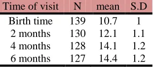
At the birth time, the average of arm circumference for boys was 10.7 cm and arm circumference for girls was 10.5 cm. So, at the birth time arm circumference in boys were 0.2 cm larger than girls. On the first visit about 2 month of age, the average arm circumference for boys was 12.7 and arm circumference for girls was 11.8 cm. In other words, within 2 month of age, arm circumference in boys was 0.9 cm larger than girls. Since speed growth rate of arm circumference in boys were different at distinct visits therefore, by analyzing data which were related to a visit, generalization those outputs to the whole period were impossible. It was similar for girls. These results are clear from Tables 1 and 2.
Table1. Mean and standard deviation of arm circumference for boys Time of visit N mean S.D
Birth time 139 10.7 1 2 months 130 12.1 1.1 4 months 128 14.1 1.2 6 months 127 14.4 1.2
Table 2. Mean and standard deviation of arm circumference for girls
Time of visit N mean S.D Birth time 148 10.5 0.8 2 months 141 11.8 1.1 4 months 129 13.5 1.1 6 months 117 13.7 1.2
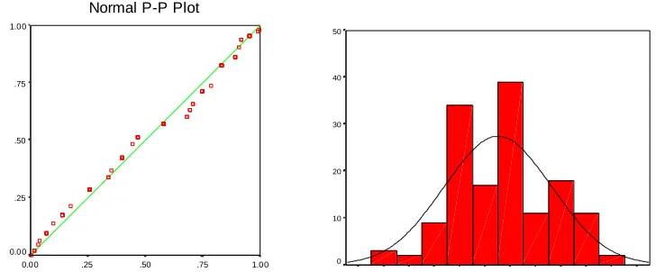
We investigated the normality of arm circumference in infants in different visits, since, in the case of normality per visit at least parametric model can be used at that occasion, therefore, we perform this investigation in all visits.
Figure 1. normality graphs for arm circumference of boys at the birth time Normal P-P Plot
1.00 .75 .50 .25 0.00 1.00
.75
.50
.25
0.00
40
30
20
10
0
IJHS 2013; 1(3): 63
Figure2. Normality graphs for arm circumference of boys at the second month of age
Figure 3. Normality graphs for arm circumference of boys at the 4th month of age
Figure 4. Normality graphs for arm circumference of boys at the 6th month of age
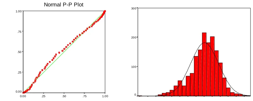
With respect to deviations from the normal distribution we can say that arm circumference in boys is not normal. About newborn girls we achieved to same results. Regardless of different visits and age of newborn at the visit time, all data were burst in a column and called newborn arm circumference. Our objective is that these data are normal or not. In other words, regardless of the time factor all the data are considered in a moment.
Normal P-P Plot
1.00 .75 .50 .25 0.00 1.00
.75
.50
.25
0.00
40
30
20
10
0
Normal P-P Plot
1.00 .75 .50 .25 0.00 1.00
.75
.50
.25
0.00
50
40
30
20
10
0
Normal P-P Plot
1.00 .75
.50 .25 0.00 1.00
.75
.50
.25
0.00
30
20
10
0
IJHS 2013; 1(3): 64
Figure 5. Normality graphs for arm circumference of boys in all visits
With regarding to deviations and skewness which have shown by Figure 5, we can conclude that the arm circumferences in boys are not normally distributed. Therefore using the parametric method is impossible. Therefore, these data can be used to evaluate nonparametric regression model that described in the previous section. But here, we will suffice to nonparametric regression model for the boys arm circumference, versus mother’s weight, mother’s arm circumference, maternal age at delivery time and maternal age at menarche. We assume that:
armc = ( )
1 t
(Mweight) + ( )2 t
(Marmc) + ( )
3 t
(Mad) + ( )4 t
(Mam)Mother’s weight (Mweight), mother’s arm circumference (Marmc) , maternal age at delivery time (Mad) and maternal age at menarche (Mam) are four independent variables and the arm circumference of infant boy is dependent variable.
We smoothed
1 , 2 , 3 ,
4 based on the time with third-degree spline smoothing method with a width of 0.67(13).
Figure 6 shows variant coefficients based on the time for mother’s weight in the above model. This figure illustrates mother’s weight effects on boy’s arm circumference when mother’s arm circumference, maternal age at delivery and maternal age at menarche are as independent variables in the model.
Normal P-P Plot
1.00 .75
.50 .25 0.00 1.00
.75
.50
.25
0.00
300
200
100
0
IJHS 2013; 1(3): 65
Figure 6. Effect of mother’s weight on boy’s arm circumference when model has four independent variables (Mweight, Marmc, Mad, Mam)
Figure 6 indicates variant coefficients based on the time for mother’s arm circumference in the model. This figure illustrates mother’s arm circumference effects on boy’s arm circumference when mother’s weight, maternal age at delivery and maternal age at menarche are as independent variables in the model.
Figure 7. Effect of mother’s arm circumference on boy’s arm circumference when model has four independent variables (Mweight, Marmc, Mad, Mam)
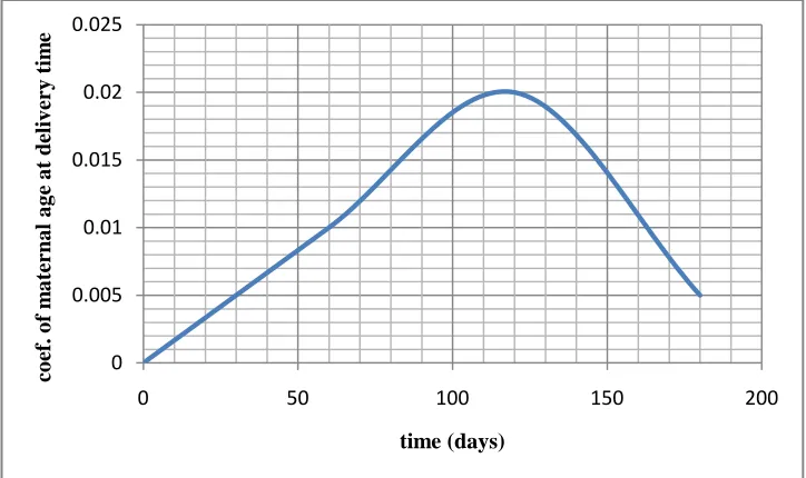
Figure 7 indicates variant coefficients based in time for maternal age at delivery time in the model. This diagram illustrate the effects of mother’s age at delivery time on boy’s arm circumference when mother’s weight, mother’s arm circumference, maternal age at menarche are as independent variables in the model
-0.06 -0.05 -0.04 -0.03 -0.02 -0.01 0
0 50 100 150 200
co
ef
.
o
f
m
o
ther
w
eig
ht
time (days)
0 0.05 0.1 0.15 0.2 0.25 0.3
0 50 100 150 200
co
ef
.
o
f
m
o
ther
a
rm
c
time(days)
IJHS 2013; 1(3): 66
Figure 8. Effect of maternal age at delivery time on boy’s arm circumference when model has four independent variables (Mweight, Marmc, Mad, Mam)
Figure 9 indicate variant coefficients based on time for maternal age at menarche in the
model. This figure illustrate the effects of maternal age at menarche on boys arm
circumference when mother’s weight, mother’s arm circumference and mother’s age at
the time of delivery are as independent variables in the model.
Figure 9. Effect of maternal age at menarche on boy’s arm circumference when model has four independent variables (Mweight, Marmc, Mad, Mam)
0 0.005 0.01 0.015 0.02 0.025
0 50 100 150 200
co
ef
.
o
f
m
a
ter
na
l
a
g
e
a
t
deliv
er
y
t
im
e
time (days)
0.4 0.5 0.6 0.7 0.8 0.9 1
0 50 100 150 200
co
ef
.
o
f
m
a
ter
na
l
a
g
e
a
t
m
ena
rc
he
time(days)
IJHS 2013; 1(3): 67
4. Discussion
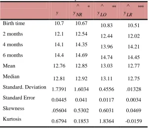
To evaluate the presented method in this section, we compared our method with linear regression (parametric) and generalized weighted regression (parametric). Linear regression (LR), generalized weighted regression (LO)and nonparametric regression (NR) were fitted to under study data when boy’s arm circumference was response variable and mother's weight, mother’s arm circumference , maternal age at delivery time and maternal age at menarche considered as independent variables. Descriptive information of fitted values on boy’s arm circumference in above models and actual values of them obtained as follows.
Table 3. Descriptive indices obtained from 3 different models and actual values of boy’s arm circumference
y
*
NR y
* *
LO y
* * *
LR y
Birth time 10.7 10.67 10.83 10.51
2 months 12.1 12.54 12.44 12.02
4 months 14.1 14.35 13.96 14.21
6 months 14.4 14.69 14.74 14.45
Mean 12.76 12.85 13.03 12.77
Median 12.81 12.92 13.11 12.75
Standard. Deviation 1.7391 1.6034 0.4556 .01328
Standard Error 0.0445 0.041 0.0117 0.0034
Skewness .05604 0.5302 0.6031 0.0469
Kurtosis 0.6794 0.1853 1.8364 -0.0159
*The fitted values of boy’s arm circumference by proposed nonparametric regression model **The fitted values of boy’s arm circumference by locally weighted regression model ***The fitted Values of boy’s arm circumference by linear regression model
y real values of boy infants arm circumference
Comparing indices of central tendency and measure of dispersion of fitted value in the three models and real values of the samples study which were located at Table3 clearly show that all indices represent the distribution of the fitted values from the model (NR) is closer than the Other fitted values . Since the model is desirable that fitted values are closer to the real values so we can be claim that the proposed model (NR) in this study for such data is better than linear regression and locally weighted regression. For further investigation, sum of squared residuals of each model could be used. The results were as follows:
SSRes (NR) =3779.37 SSRes (LO) = 4510.14 SSRes (LR) =4585.79
IJHS 2013; 1(3): 68
Thus proposed nonparametric regression (NR) not only has similar distributions with real data distribution of boy’s arm circumference, but also it has lowest sum of squared residuals in comparison with linear regression and locally weighted regression. This means that the fitted values represented by proposed nonparametric regression model compared to other models is closer to the true values. In order to evaluate the appropriateness of models, normality tests for residuals of models were used. Graphical approach was used for this objective, so histograms and pplot for the residuals of models drawn.
3 00
2 00
1 00
0
Normal P-P Plot
1.00 .75
.50 .25
0.00 1.00
.75
.50
.25
0.00
Figure 10. Normality graphs for residuals of proposed nonparametric regression model (NR)
300
200
100
0
Normal P-P Plot
1.00 .75
.50 .25
0.00 1.00
.75
.50
.25
0.00
Figure 11. Normality graphs for residuals of linear regression model (LR)
IJHS 2013; 1(3): 69
300
200
100
0
No rmal P-P Pl ot
1 .00 .7 5
.5 0 .2 5
0 .00 1 .00
.7 5
.5 0
.2 5
0 .00
Figure 12. Normality graphs for residuals of locally weighted regression (LO)
With comparing Figure 10,11 and 12, it will be obvious that only residuals of nonparametric regression (NR) is normally distributed and residuals obtained from locally weighted regression and linear regression models showed a significant deviation from the normal distribution. Since the normality of residuals is a basic condition for the suitability model, these plots are another reason for preferring non-parametric regression models with time-dependent coefficients in comparison to other two models. So the proposed nonparametric regression with varying coefficients could be recommended for longitudinal data.
References
1.Faraway J. Human Animation Using Nonparametric Regression. Journal of Computational and Graphical Statistics. 2004;13(3):537-53.
2.Lin DY, and Ying, Z. Semiparametric and Nonparametric Regression Analysis of Longitudinal Data. Journal of the American Statistical Association 2001;96:103-13.
3.Wu CO, Yu, K.E., and Chiang , C.T. . A Two - Step Smoothing the method for Varying - Coefficient Models with Repeated Measurments. The Annals of Institute of Statistical Mathematics 2000;53:519-43.
4.Wu CO, Yu, K.E., and Yuan, W.S. Large - Sample Properties and Confidence Bands for Component - Wise Varying - Coefficient Regression with Longitudinal Dependent Variables Communication Statistics 2000;29:1017-37.
5.Yao W, Li R. New local estimation procedure for a non-parametric regression function for longitudinal data. Journal of the Royal Statistical Society. 2013;75(1):123-38.
6.Kovac A, Smith A. Nonparametric Regression on a Graph. Journal of Computational and Graphical Statistics. 2011;20(2):432-47.
7.Diggle PJ, Liang, K.Y., and Zeger, S.L. Analysis of Longitudinal Data: Oxford University Press 1994.
8.Payandeh A, Saki A, Safarian M, Tabesh H, Siadat Z. Prevalence of Malnutrition among Preschool Children in Northeast of Iran, A result of a Population based Study. Global Journal of Health Science. 2013;5(2):208-13.
9.Durban M, Harezlak J, Wand MP, Carroll RJ. Simple fitting of subject-specific curves for longitudinal data. STATISTICS IN MEDICINE. 2004:1-24.
IJHS 2013; 1(3): 70
10.Payandeh A, Tabesh H, Shakeri MT, Saki A, Safarian M. Growth Curves of Preschool Children in the Northeast of Iran: A Population Based Study Using Quantile Regression Approach Global Journal of Health Science. 2013;5(3):9-15.
11.Hardle W. Applied Nonparametric Regression London: Cambridge University Press 1994.
12.Song X, Mu X, Sun L. Regression Analysis of Longitudinal Data with Time-Dependent Covariates and Informative Observation Times. Scandinavian Journal of Statistics. 2012;39:248-59.
13.Huang J, Win C, Zhou L. Polynomial Spline Estimation And Inference For Varying Coefficient Models With Longitudinal Data. Statistica Sinica. 2004;14:763-88.
14.Saki A, Eshraghian M, Mohammad K, RahimiForoushani A, Bordbar M. A prospective study of the effect of delivery type on neonatal weight gain pattern in exclusively breastfed neonates born in Shiraz, Iran. International Breastfeeding Journal. 2010;5(1).
15.Saki A, Eshraghian M, Tabesh H. Patterns of Daily Duration and Frequency of Breastfeeding among Exclusively Breastfed Infants in Shiraz, Iran, a 6-month Follow-up Study Using Bayesian Generalized Linear Mixed Models. Global Journal of Health Science. 2013;5(2):123-33.