Second-Order Statistical Texture Representation of Asphalt Pavement Distress Images Based on Local Binary Pattern in Spatial and Wavelet Domain

DOI: 10.22075/JRCE.2018.14785.1272

Journal homepage: http://civiljournal.semnan.ac.ir/

Second-Order Statistical Texture Representation of

Asphalt Pavement Distress Images Based on Local

Binary Pattern in Spatial and Wavelet Domain

R. Shahabian Moghaddam1, A. Mohammadzadeh Moghaddam1, S.A.

Sahaf1 and H.R. Pourreza2

1. Department of Civil Engineering, Ferdowsi University of Mashhad, Mashhad, Iran. 2. Department of Computer Engineering, Ferdowsi University of Mashhad, Mashhad, Iran.

Corresponding author:[email protected]

ARTICLE INFO ABSTRACT

Article history:

Received: 10 March 2018 Accepted: 12 June 2018

Assessment of pavement distresses is one of the important parts of pavement management systems to adopt the most effective road maintenance strategy. In the last decade, extensive studies have been done to develop automated systems for pavement distress processing based on machine vision techniques. One of the most important structural components of computer vision is the feature extraction method. In most of the application areas of image processing, textural features provide more efficient information of image regions properties than other characteristics. In this research, three different algorithms were used to extract the feature vector and statistically analyzing the texture of six various types of asphalt pavement surface distresses. The first algorithm is based on the extraction of images second-order textural statistics utilizing gray level co-occurrence matrix in spatial domain. In second and third algorithms, the second-order descriptors of images local binary patterns were extracted in spatial and wavelet transform domain, respectively. The classification of the distress images based on a combination of K-nearest neighbor method and Mahalanobis distance, indicates that two stages arranging of the gray levels of the distress images edges by applying wavelet transform and local binary pattern (third algorithm) had a superior result in comparison with other algorithms in texture recognition and separation of pavement distresses. Classification performance accuracy of the distress images based on first, second and third feature extraction algorithms is 61%, 75% and 97%, respectively.

Keywords:

Pavement Distress Texture, Computer Vision,

Gray Level Co-Occurrence Matrix (GLCM),

1. Introduction

In Iran, which more than 90% of freight and passenger transportation is relied on overland transport network, the road network has a pivotal role in country's wealth and must be fully capable of preserved [1]. To determine the apropos (economic) road treatment, the pavement management system (PMS) must be implemented. Pavement evaluation is one of the most significant elements of pavement management systems. Pavement assessment includes a range of qualitative and quantitative measurements to determine the operational and structural pavement conditions. Collecting the pavements assessment data is in terms of four sections including serviceability, structural capacity, surface failure (pavement distress) and safety (fraction). Identification and tracking of road surface distresses are considered as one of the main parts of the pavement performance assessment process at all levels of road management. In addition, one of the primary reasons for reducing road serviceability is pavement distresses [2]. Basically, manual (visual) methods are administrated to determine and measure the pavement distresses. Experiences has shown that this pavement scoring approach, despite its high accuracy, costs a considerable amount of time and money. It is also dependent on evaluator’s personal judgments (subjective) and will lead to unstable results. In the last decade, in order to fix the visual distress assessment defects, comprehensive researches has been done to develop semi-automated and fully-automatic methods of pavement inspection. In full-automated pavement assessment, all stages of gathering and processing distress date are done without or very few human intervention [3, 4].

classification of these images based on decision tree learning method, resulted in about 35% errors. In the aforementioned research, in addition to using a large number of features and high computing loads, the GLCM has been formed unidirectional and symmetrically. Whiles, locating distribution of the distress gray levels should be analyzed in different directions by considering the order of pixel placement (non-symmetric GLCM) Lee [8] used the histogram statistical moments of the Fourier coefficients to analyze the texture of various types of pavement surface cracks. Afterwards he performed the support vector machine classifier to discriminate the images. The result of classification accuracy rate was about 72%. Fourier transform not only doesn’t provide sparse information of the distress images important information, such as edges, but also only preserves the frequency data of the signal and the locative resolution is completely disappeared. It should be noted that to distinguish different patterns of pavement distresses, such as longitudinal and transverse cracks, both frequency spectrum and the spatial information are necessary. Zou et al. [9] performed image enhancement techniques like histogram improvement and Fourier transformation to preprocess the images, and used the artificial intelligence and machine learning techniques, such as neural networks, to classify them. Finally they reported about 25% of errors in image categorization. Wang [10] implemented gray level gap length matrix statistics in Fourier and wavelet domain to extract the texture feature vector of various types of asphalt pavement surface cracks, and used minimum Euclidean distance to discriminate the images.

The images classification accuracy in the frequency domain (Fourier transform) and

the frequency-spatial domain (wavelet transform) was reported 64% and 76% respectively. It should be noted that the distresses texture features are interrelated and dependent, and Euclidean distance is not able to consider these correlations. Moghadas nejad and Zakeri [11] used a fusion of the first and second order texture features (18 features) in Haar, Coiflet 6 and Curvelet domains and employed dynamic neural network for the purpose of classifying 7 types of asphalt pavement crackings including: block cracks, alligator cracks, whisker (hair) cracks, longitudinal cracks, transverse cracks, diagonal cracks and multiple cracks. It should be mentioned that preprocessing and image enhancement techniques such as histogram modification were also implemented in the article. In the end, in the domain of Haar, Coiflet 6 and directional selective Curvelet transforms, about 4%, 15% and 2% of classification errors were reported respectively. Ouyang et al. [12] used various methods of feature space dimension reduction (feature selection) to form a representative texture feature vector in Daubechies wavelet transform domain. In the mentioned research, three layers of wavelet decomposition and averaging between horizontal, vertical and diagonal details sub-bands were used in different ways and the results were compared. In 2016, all methods of semi-automatic and all-semi-automatic acquiring and processing asphalt pavement distresses were reviewed [4].

affect the proposed repair options suggested by PMS. Previous algorithms that reported less than 5% of classification errors often have a heavy and fairly complex computing load (Image preprocessing, using directional selective transforms with high redundancy, great number of features, complex classification algorithm, etc.) which leads to time and cost increasing of the pavement performance evaluating. In image transition from spatial domain to transformation domain, we need to utilize a transformation in which the important information and image edges be present in specified sub-bands and not be dispersed. Since The important (discriminator) information and components of the asphalt pavement distress images include horizontal and vertical (non-directional) edges, as shown in fig. 1, the directional sensitivity of two-dimensional discrete wavelet (horizontal, vertical and diagonal) is appropriate and adequate

(non-dispersion distress data). In such patterns it is better to concentrate on the type (shape) and scale (number of analyzing layers) of the applied wavelet and feature extracting procedure than focusing on increasing the directional sensitivity of the transformation (Such as implementing Curvelet transform). In this study, with a review of many previews studies in analysis and classification of various texture types, a few features (4 second-order texture descriptors) with the highest power of differentiation were selected to describe the asphalt distresses local patterns texture in spatial and wavelet domain. Furthermore, a simple classification method were performed to categorize the data. The algorithm presented in this study, despite the simplicity and low computational load in compare with previous methods, has higher accuracy in recognizing and discriminating pavement distresses.

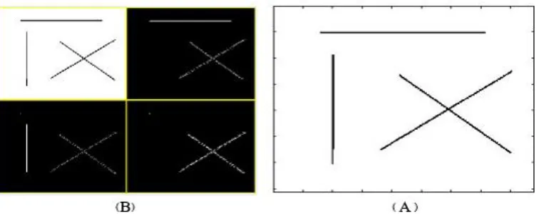
Fig. 1. A. An image That includes linear horizontal, vertical, and diagonal discontinuities (singularities) / B. pyramid resultant of applying one layer Haar discrete wavelet decomposition on image A [18]. As shown in fig. 1, the structural details of

horizontal and vertical edges are summarized in specified sub-bands, but the diagonal components information of the image are scattered in all sub-bands.

Utilizing 3D laser imaging (scanning) systems is not an optimal and economical

images. Briefly, in most of the automatic pavement distresses evaluation systems, there is no difficulty in procurement the required data. The main defect and limitation is in full-automatic and efficient distress data analysis (process) [13]. This research focuses on asphalt pavement distress images analysis and pattern recognition algorithms. It should be mentioned that, although the main focus of this study is on identifying and differentiating various types of asphalt pavement distress patterns, in pavement management systems, measuring distresses extent and intensity are of great importance.

Automated processing of pavement distress images is often based on machine vision systems and computer algorithms. Data acquisition, image enhancement, segmentation, feature extraction and pattern recognition can be mentioned as the main components of these systems. Extracting the image features is actually the transformation of input data into a series of useful details and is considered one of the most substantial components of the machine vision systems in the process of classification and identifying the image pattern [14]. Extracted features from the image such as color, texture, moment invariants and geometric features (shape) are often in numeric formatting and are considered as image representative. In pattern recognizing and classifying process, we must try to extract the same features of same classes, which, at the same time, are different and distinct from the other categories features. Compared with the other features, textural characteristics provide more comprehensive information of the image properties, and have a superior performance in many applications, such as medical image analysis, classification of radar images, face recognition, fingerprints and especially in

recognizing and separating various distresses patterns [15].

2D wavelet transform, analyze the image

texture structures in horizontal, vertical, and diagonal directions.

Fig. 2. Time (spatial) and frequency resolutions in multi-resolution wavelet transform. Distresses observed on the pavements, are divided in two main families including fundamental and functional distresses. According to the pavement distress evaluation and identification manuals such as ASTM D6433, LTPP, and etc., among the most important fundamental distresses of asphalt pavement, fatigue (alligator) cracks, longitudinal and transverse cracks can be mentioned. Patching, bleeding and raveling are of the main functional distresses

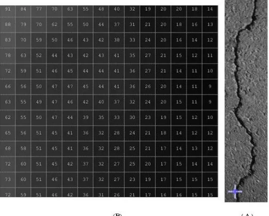
generated on asphalt pavement surfaces [18]. In addition to the mentioned distresses, undamaged (without failures) asphalt images were also analyzed in this research. Thus, the acquisitions of asphalt pavement surface were classified into seven different groups. It should be mentioned that measuring the extent and severity of different distresses often differs in various distress assessment manuals and are mostly the same in their definition and recognition. The main problems of the automated distress classifying algorithms are in severe disorders in distress texture gray levels. In other words, although the general pattern of gray level values alternations are alike in edge areas in same classes, but there is no regular local connection between pixel values. The main result for this disorderly is the creation of distresses on the pavement surface under variable loading and atmospheric conditions. For example, a sample of an 8-bits image of a longitudinal crack along with the gray level value matrix of the specified zone is shown in Figure 3.

As shown in Figure 3, there is a few spatial relation and interaction between the distress image gray levels in spatial domain. These irregularities cause the lack of extracting same features for the same classes and chase the loss of the accuracy in recognition and discrimination of image texture patterns. In this study, two different algorithms were used in order to regulate and analyze the distresses texture. Regularization in the first algorithm is based on local binary pattern formation of the image. The most important property of the local binary pattern operator, which leads to regularization of gray levels, is resisting to the changes of the values of the image intensity levels [19]. In the second algorithm, local binary pattern features of distress images were used in the wavelet domain. In other words, the second algorithm uses two levels of distress texture regularization based on wavelet transform and local binary pattern and investigates the local patterns of image frequency contents. In transforming the image from spatial domain to wavelet domain, the similarity (proximity) is measured with the wavelet function pattern [20]. Therefore, in forming the frequency-spatial content of the image (wavelet coefficients) the irregularities of gray levels, which exist in spatial domain distress textures, are greatly reduced. Moreover, a spatial distress texture analysis algorithm is used to investigate the efficacy of performing the mentioned regularization algorithms. The image gray levels, texels and frequency content of most asphalt pavement distresses have a specific local relation with each other. Therefore, in this study, in order to analyze the distresses texture and extract the images feature vector, second-order statistics based on Gray Level Co-occurrence Matrix (GLCM) were used. Although histogram measurements provide useful information of

the texture components abundance, it does not provide any information about the relation and the local interaction between them. GLCM, unlike the intensity histogram, is calculated and extracted regarding the relationship and location between 2 pixels, and is sensitive to image pixels displacement [21]. Finally, utilizing the calculated statistical texture descriptors, distress images are categorized according to the K-nearest neighbor (KNN) classifier and the classification performance is evaluated by two indicators: sensitivity and accuracy.

2. Theoretical Concepts

In this part of the study, the theoretical foundations of discrete wavelet transform (DWT) and local binary pattern (LBP) are presented along with the basic concepts of the GLCM statistical descriptors.

2.1. Discrete Wavelet Transform (DWT)

DWT is the decomposition of a signal into a set of child-wavelet functions 𝜑_𝑚𝑛(𝑡) that are obtained in accordance with equation 1 by translating and scaling the mother-wavelet function φ(𝑡).

𝜑_𝑚𝑛(𝑡) = 2−𝑚⁄2 _𝜑(2−𝑚_{𝑡 − 𝑛)} (1)

Where m and n are indexes related to the scaling (decomposition level) and translation (shift).

The mother-wavelet function is driven from the scale function ϕ(𝑡) according to equations 2 and 3.

𝜙(𝑡) = √2 ∑𝑘𝜖ℤℎ0(𝑘)𝜙(2𝑡 − 𝑘) (2)

𝜑(t) = √2 ∑_𝑘𝜖ℤℎ₁(𝑘)𝜙(2𝑡 − 𝑘) (3)

In which h0 and h1, represent the low pass

respectively, and are different according to being from which wavelet family. [22]

In practical applications, we don’t directly address the wavelet and scaling function, in fact low pass and high pass filters are employed to apply the wavelet transform and decompose the signal. The low pass filter output is approximation sub-band that includes signal low-frequency information and the high pass filter output is detail sub-bands that contain high-frequency components of the signal. Depending on the

required or desired frequency resolution, decomposition of the sub-band resultant from signal low pass filtering can be repeated and generate the sub-bands of different layers of wavelet decomposition [23,24].

For applying DWT on image (2D) signals, two dimensional wavelet transform should be used. For this purpose, one dimensional wavelet transform is applied to the rows and columns of the image matrix, respectively. The mentioned process is represented in Figure 4.

Fig. 4. One-layer diagram of image (2D) wavelet decomposition [23].

In each level of decomposition, the image I(x,y) is passed through the low pass filter and high pass filter along with the rows, and is sub-sampled. At this stage, two images are obtained that one of them includes the low frequencies of the image IL(x,y) and the other

one contains the high frequencies of it IH(x,y). In the next step, the filtering of each

of these two sub-images is done along with the columns and is sub-sampled. As a result, four sub-images (sub-bands) are obtained, which are:

_ The ILL sub-band that is correspondent to

the image low-frequency components. This sub-band contains the original image

generalities, and is known as the wavelet approximation coefficients matrix.

_ High frequency sub-band ILH that contains

the image horizontal details (edges).

_ High frequency sub-band IHL that contains

the image vertical details (edges).

_ High frequency sub-band IHH that contains

the image diagonal details (edges).

(discriminative) information of the image, are the high frequency components. The extracted features of these sub-bands, in other words, studying of the distribution of the wavelet coefficients (image frequency content) can efficiently describe the image texture [25].

Each family of the wavelets, has its own unique mother scaling and wavelet functions. In this study, the Haar wavelet was used to extract the edges and analyze the asphalt distresses. The reason for choosing this wavelet is the less supported window width (related to the number of employed adjacent

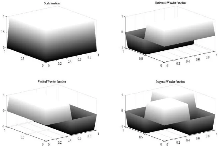
pixels in order to extract the wavelet coefficients) in compare with other wavelet functions. Because of the texture severe irregularities of the asphalt pavement distress images, importing a large number of pixels in extracting wavelet coefficients is not correct. This could be attributed due to the increasing possibility of absorbing the irregularities. The support width (window) of the Haar wavelet is 1 and it uses weighted average of two adjacent pixels in order to extract the distress edges [26]. The 3D schema of the Haar wavelet and scaling functions is shown in Figure 5.

Fig. 5. Scale function and horizontal, vertical diagonal detail functions of 2D Haar wavelet.

2.2. Local Binary Pattern (LBP)

In recent years, the application of local binary pattern has increased significantly in the field of computer vision and image texture process. In summary, the local binary pattern, as a non-parametric method, efficiently represents image local structures by comparing each pixel with the adjacent pixels. Two of its most important properties

is its resistance to the variations of the image gray levels and its computational simplicity. LBP is known as a powerful approach for analyzing the texture and describing the image local structures and frequency sub-bands [19].

this research the neighborhood is considered as square. This method was first proposed by Ujela as a 3*3 square operator. The mechanism of this method is comparing 8 neighbors on the operator with the central pixel. Each of these 8 pixels is replaced by 1 if its value is equal or greater than the value of the central pixel. Otherwise its value will be 0. In the end, the central pixel value is

replaced by binary weighted summing of the neighbor pixels and the 3*3 window will be transferred to the next pixel [27]. In Figure 6, the operator operation of the LBP is displayed. By forming the GLCM of the obtained values and extracting second-order statistics, the image texture could be efficiently analyzed.

Fig. 6. LBP operator in order to describe the image texture.

2.3. Gray Level Co-occurrence Matrix

(GLCM)

GLCM was first introduced by Haralick. This matrix can be defined in various angles (directions) and various pixel intervals, each of which somehow describes and presents texture properties. For GLCM based feature extraction, the probability density function G (I,J|D,θ ) should be generated. To calculate the probability density function, we should count the pair of pixels with i and j gray levels, which are located at d distance and at θ angle from each other [28]. GLCM is calculated according to equation (4).

𝑃_𝑑,𝜃(𝑥, 𝑦) = ∑ ∑𝑀−1𝑔(𝑖, 𝑗) = 𝑥, 𝑔(𝐼, 𝐽) = 𝑦

𝑗=0 𝑁−1

𝑖=0 (4)

In equation 4, M and N represent the number of image pixels in the horizontal and vertical directions, respectively. g(i,j) is the pixel gray level at (i,j) and g(I,J) is the pixel gray level value in the position (I=i+r, J=j+r). r is

the distance between 2 pixels that are located in θ angle and D distance. In most researches, after normalizing the matrix, in order to describe and statistically analyze the image (or sub-band) texture, 4 important features of the GLCM, which are contrast, correlation, energy, and homogeneity are used. The equations and description of these statistics are presented in reference [18].

3. Research Process and Validation

of the Proposed Texture Analysis

Algorithms

The process of the research consists of five main steps:

1- Image acquisition of asphalt distresses under controlled conditions.

2- Extracting the images texture feature vector based on the proposed algorithms.

3- Classifying the distress images (pattern recognition)

4- Evaluation of the algorithms performance

5- Results and discussion

3.1. Image Acquisition of Asphalt

Pavement Distresses

In this study, a hardware (in accordance with the Figure 7) was used in order to capture the distress pictures in high quality and controlled lighting conditions. This hardware eliminates the necessity of image pre-processing operations using complete deletion of the ambient light by tarpaulin and providing artificial lighting (lamp) with constant intensity and certain distances of asphalt pavement surface for all acquisitions. It should be mentioned that all distress images were taken in the same condition with a 14-megapixels resolution Fujifilm digital camera from 1 meter height of asphalt surface (no zooming in), and then were transferred from color type to the monochromic with dynamic range of 0 to

256 (8 bits). As the extent and intensity of the distresses in the images increases, the discrimination power of different texture patterns increases. It should be reminded that the suggested texture analysis algorithms, are based on the number and local interaction of the distresses image gray levels and are not

dependent on the location of the distress in the image. It’s worth mentioning that imaging in the absence of intense sunlight (in afternoon), when the negative effects of shadows are minimized, has the most similarity to the controlled lighting conditions. This matter is important in the executive implementing of the automated pavement distress evaluation systems. Furthermore, it is recommended to use linear scanning digital cameras for taking images. In this case, problems caused by images discontinuity and overlapping are minimized.

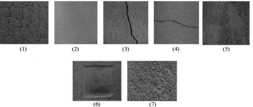
Fig. 7. The hardware used for pavement distress image capturing in controlled conditions. The acquired images of pavements were classified into 7 groups (as shown in Figure

8) including:

Fig. 8. Classification of the acquired distress images: 1. Alligator (fatigue) cracking 2. Without distress 3. Longitudinal cracking 4. Transverse cracking 5. Bleeding 6. Patching 7. Raveling.

3.2. Statistical Texture Analysis of the

Distress Images

In the present study, 3 algorithms were used to extract the texture features. The first algorithm is based on extraction of the image GLCM statistics in spatial domain. In second algorithm, first, the LBP of the distress image is composed and then, the GLCM features of these patterns are calculated. In the third algorithm, first the wavelet transform is applied to the image, then the LBP of the wavelet coefficients (frequency-spatial contents of the image) are extracted. At the end, GLCM based second-order statistical descriptors organize the feature vector elements.

3.2.1. Extracting the Feature Vector Based on GLCM in Spatial Domain

In this algorithm (first algorithm), the image second-order statistics were directly extracted via distress image gray levels. In this research, GLCM dimension is 265, the interval (offset) parameter is 1, and according to different spatial distribution of gray levels in distress patterns, 4 distinct angles (0°, 45°,

90°, 135°) were selected as the direction parameter to form the asymmetric GLCM.

After normalizing the GLCM values of the distress images, second-order statistics including contrast, correlation, energy and homogeneity) are severally extracted in each of the four selected directions and their average is calculated as the final measurements. These final statistical descriptors, form 4 entries of the image feature vector. This vector, is considered as the distress image texture representation in the classification process.

3.2.2. Extraction the Feature Vector Based on Second-Order Statistics of the Image LBP

3.2.3. Extraction the Feature Vector Based on Image Frequency Content LBP Second-Order Statistics

In this algorithm (third algorithm), first, the distress images are decomposed by applying two layers of Haar wavelet transform. Then, the LBP of image detail (high-frequency) sub-bands forms and finally the second-order statistics of these local patterns are calculated based on normalized GLCM. In other words, in this algorithm, the distribution and spatial interaction between the local patterns of the wavelet coefficients (frequency-spatial content of the distress images) are analyzed. It is worth mentioning that, since the main and important information of the distress images (i.e. edges) are placed in high-frequency sub-bands, only the wavelet details coefficients matrices are analyzed. It should be noted that by increasing the number of wavelet decomposition levels, despite the increase in the frequency accuracy, the

locality (spatial resolution) of the image texture components decreases. The optimized number of wavelet decomposition level in order to extract and reveal the structural details of the texture of the pavement distress images is 2 [29].

In this algorithm, after applying two levels of

2D Haar DWT on the distress images and

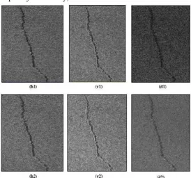
extraction of the detail coefficient matrices, including: first layer horizontal details band (H1), first layer vertical details band (V1), first layer diagonal details sub-band (D1), second layer horizontal details sub-band (H2), second layer vertical details sub-band (V2), second layer diagonal details band (D2), the LBP (L) of these six sub-bands (sub-images) has been formed. For example, the details sub-bands of applying two layers 2D Haar wavelet decomposition on longitudinal cracking (Figure. 7-3) are presented in Figure 9.

Fig. 9. Applying two-layer Haar DWT and extracting structural details of longitudinal cracking texture.

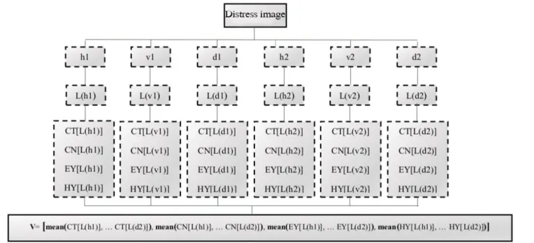
In the next step, the GLCM of images high frequency sub-bands LBP are calculated in

matrices including: Contrast (CT), Correlation (CN), Energy (EY) and Homogeneity (HY) formed the feature vector of each sub-band. The arithmetical average (mean) of peer to peer bands (6

sub-bands) statistics, generates 4-final elements of the distress image feature vector (V). The process of extracting the texture feature vector of the images based on this algorithm (third algorithm) is presented in Figure 10.

Fig. 10. The algorithm of distress image feature vector extraction based on second-order statistics of wavelet sub-bands local patterns.

3.3. Classification of Distress Textures Classification refers to the process of mapping an unknown datum to a set of predefined groups, and is one of the most important applications of supervised machine learning [30]. K nearest neighbor (KNN) is the classifier of this research. In this method, in the training stage, all samples of the geometric space are multi-dimensional vectors. It should be mentioned that, in this research, the dimension of the feature space (the number of the feature vector elements) is 4. In the present study, Mahalanobis distance (d) is used as a criterion for determining the new sample (testing image) class in accordance with equation 5.

d 2 _{= (p – k}

c) Cc-1 (p – kc) T (5) In this equation, p is the feature vector of the testing image, and kc is the feature vector of one of the training images of c distress class. Cc represents the covariance matrix of the feature set of the learning images of the c class. The advantage of using Mahalanobis

distance into Euclidean distance is to spot the relations and correlation between the entries of the feature vectors by computing the covariance of the features, which results in accuracy enhancement of the classification [31]. It should be recalled that the number of classes in this research is 7 and each class has

60 images that 30 of them are selected as the training data, and the other 30 pictures are elected as testing data.

classes are triangle, which is considered as the class of the testing sample. In this research the criterion for distance measurement is Mahalanobis, and it has been proved that the optimized K quantity, according to the cross-validation method, is 3 for the distress data [18].

Fig. 11. Class determination of the testing sample using KNN method [30].

3.4. Performance Evaluation of the

Distress Images Classification.

The confusion matrix is a square matrix and represents how the testing images are allocated to different distress classes. Dimensions of this matrix is equal to the exiting classes, and its diagonal entries expresses the correct assignment of the

distress image to the related category. In this study, in order to evaluate the performance of each feature extraction algorithm in automated classifying of asphalt pavement distress images, two indicators including sensitivity and accuracy were measured. Sensitivity and accuracy rates are of the most important extracted indicators of the confusion matrix to evaluate the classification (statistical pattern recognition) performance [32].

Sensitivity (SN) expresses the classifier ability in correct identifying of each class images, and is calculated according to equation (6).

𝑆𝑛𝑔= 𝑛𝑔𝑔

𝑛𝑔 (6) In this equation 𝑛𝑔𝑔 is the number of testing images belonging to category G, that is correctly assigned to the corresponded class (the diagonal elements of the confusion matrix) and 𝑛𝑔 represents the total number of category G data (the sum of each row entries). It should be reminded that in this research, the 𝑛_𝑔 parameter is equal to 30. In table 1, the sensitivity rates of feature vector extraction algorithms in automated classification of asphalt distress images are presented

Table 1. Sensitivity rates of classifying pavement distress images based on proposed texture analysis algorithms.

DWT+LBP+GLCM LBP+GLCM

GLCM Algorithm

Distress type

0.9 0.47

0.3 Alligator cracking

1 0.93

0.83 Without distress

0.97 0.63

0.47 Longitudinal cracking

0.97 0.7

0.53 Transverse cracking

0.93 0.53

0.37 Bleeding

1 0.97

0.9 Patching

1 1

Accuracy (Ac) represents the general performance of the algorithm in classifying of the images, and is extracted from the testing images confusion matrix, according to equation 7. In other words, the accuracy is equal to the average of the sensitivity of classifying all distress groups.

𝐴𝑐 =∑ 𝑛𝑔𝑔

𝐺 𝑔=1

𝑛 (7) In this equation 𝑛𝑔𝑔 is the number of testing images belonging to category G that is

correctly assigned to the corresponded class (the diagonal elements of the confusion matrix). G is the number of classes and n denotes the total number of testing images (total amount of confusion matrix elements). It should be reminded that in the present research, G and n are equal to 7 and 210, respectively. In Figure 12, the accuracy rates of the 3 proposed algorithms in classification of the texture of the asphalt distress images is presented.

Fig. 12. Accuracy rates of the asphalt pavement distresses classification based on the proposed texture analysis algorithms.

3.5. Discussion and Results

- The created distresses the asphalt pavement surface are highly irregular and the gray levels creating their image textures, have a random modality in micro viewpoint. The reason for these irregularities, in addition to the heterogeneous texture of pavement materials, is the strong dependence of distress formation to the climate conditions and traffic volumes. In one class of distresses, although the general pattern of the image texture is similar, there is a poor spatial relation between the gray levels of the

second-order statistical descriptors (first algorithm) is 61%.

- As regards the LBP is invariant into the changes in illumination intensity values (gray levels) of the image pixels, and is extracted and calculated based on general comparison (More or less) values of neighbor pixels, arranges the texture of the distress image. Furthermore, wavelet coefficients (image frequency contents) are a measurement of the similarity (matching) of the original signal with the wavelet function. The result of this similarity quantification, is the calculation of the weighted average of the image gray levels and hereupon the regularization of the distress edge textures. Extraction the texture feature vector of the image based on second-order statistics of image local patterns (second algorithm) yielding 75% classifying accuracy, obtained a better performance in identifying the distresses into the spatial analysis of the distresses texture (first algorithm). The statistical texture analysis of distress images by means of GLCM of the local patterns of the image frequency content (third algorithm), since it double regularizes the image gray level values in, has a superior result in recognizing and discriminating distress textures than the first and the second algorithms. By performing the third algorithm, 97% of captured distress images,

assigned to the relevant class correctly.

- Although the general patterns of longitudinal and transverse cracks are similar and all utilized texture analysis algorithms in this research obtain a partly close classification sensitivity in recognizing these two kind of distresses, these two failures are not merely the rotated form of each other and difference incidence in classification sensitivity of these distress classes is inevitable. The reason of this matter is the

difference in the irregularities quantity in the images of these two distresses along with severe sensitivity of texture analysis algorithms to these irregularities. The differences between classification sensitivity rates of longitudinal and transverse cracks based on all applied texture analysis algorithms in this research, is less than 8%.

- The texture analysis algorithms, used in this study, have high sensitivity rates in classifying reveling and intact asphalt (without distress) classes, because the values and the distribution of gray levels of these classes, form a completely rough texture (due to the repeated changes of the values of the gray levels from tar and aggregates) and a completely smooth (soft) texture, respectively. Their texture pattern contains less irregularities. It should be mentioned that, if there be a regularity in the gray level values of the image texture, the local patterns and the image frequency contents (wavelet coefficients) will also have a regular patterns, consequently. It worth reminding that texture regularity, causes the extraction of similar features from the same patterns, and increase the recognition accuracy of the distresses.

identifying it. The average sensitivity rate of classifying patching based on proposed texture description algorithms in this research is 96%.

- Although, studying the spatial interaction between the local patterns of image frequency content (third algorithm) having classification accuracy of 97%, has a superior performance than other algorithms in discriminating pavement distress textures, it should be noted that employing wavelet transform, increases the computational loads of the image processing algorithm. Increment in the algorithm computational loads leads to an increase in image analyzing time and cost. Considering that we are faced with a considerable amount of data in mapping the pavement information, the quantity of computational loads of the image analysis algorithm has a particular importance. Therefore, making decisions related to choosing the analysis method and the used processing algorithm in automated pavement evaluating systems, is dependent on the requisite accuracy rate, time and budget limitation of road assessment project and the manager’s opinion.

REFERENCE

[1] Khodakarami, M., Khakpour Moghaddam, H. (2017). 'Evaluating the Performance of Rehabilitated Roadway Base with Geogrid Reinforcement in the Presence of Soil-Geogrid-Interaction', Journal of Rehabilitation in Civil Engineering, 5(1), pp. 33-46.

[2] Shahabian Moghaddam, R., Sahaf, S. A., Mohammadzadeh Moghaddam, A., Pourreza, H. R. (2018). 'Automatic Recognition and Classification of Pavement Distress based on Analysis of Image Texture in Spatial and Transformation Domain', Quarterly Journal

of Transportation Engineering, 9 (special), pp. 121-142.

[3] Wang, K. C. P., Li, Q. J., Yang, G., Zhan, Y. and Qiu, Y. (2015) “Network level pavement evaluation with 1 mm 3D survey system”, journal of traffic and transportation engineering, Vol. 2, No. 6, pp. 391-398.

[4] Zakeri, H., Moghadas Nejad, F. and Fahimifar, A. (2016) “Image based techniques for crack detection, classification and quantification in asphalt pavement: a review”, Archives of Computational Methods in Engineering, pp. 1-43.

[5] Chua, K. M. and Xu, L. (1994) “Simple procedure for identifying pavement distresses from video images”, Journal of Transportation Engineering, Vol. 120, No. 3, pp. 412-431.

[6] Nallamothu, S. and Wang, K. C. P. (1996) “Experimenting with recognition accelerator for pavement distress identification”, Transportation Research Record, Vol. 1536, pp. 130-135.

[7] Cheng, H. D., Glazier, C. and Hu, Y. G. (1999) “Novel approach to pavement cracking detection based on fuzzy set theory”, Journal of Computing in Civil Engineering, Vol. 13, No. 3, pp. 270-280. [8] Lee, D. (2003) “A robust position invariant

artificial neural network for digital Pavement crack analysis”, Technical report, TRB Annual Meeting, 2009, Washington, DC, USA.

[9] Zou, Q., Cao, Y., Li, Q., Mao, Q. and Wang, S. (2008) “Crack-tree: automatic crack detection from pavement images”, Pattern Recognition Letters, Vol. 33, No. 3, pp. 227–238.

[11] Moghadas Nejad, F. and Zakeri, H. (2011) “A comparison of multi-resolution methods for detection and isolation of pavement distress”, Expert Systems with Applications, Vol. 38, No. 3, pp. 2857-2872.

[12] Ouyang, A., Dong, Q., Wang, Y. and Liu, Y. (2014) “The classification of pavement crack image based on Beamlet algorithm”, in: 7th IFIP WG 5.14 international conference on computer and computing technologies in agriculture, CCTA 2013. [13] Moghadas Nejad, F. and Zakeri, H. (2011)

“An optimum feature extraction method based on Wavelet–Radon Transform and Dynamic Neural Network for pavement distress classification”, Expert Systems with Applications, Vol. 38, No. 3, pp. 9442-9460.

[14] Gonzalez, R.C. and Woods, R.E. (2006) “Digital image processing 3/E”, Prentice Hall, Upper Saddle River, NJ, USA. [15] Srinivasan, G. N. and Shobha, G. (2008)

“Statistical texture analysis”, proceedings of world academy of science, engineering and technology, No. 36, pp. 207-213. [16] Aggarawal, N. and Agrawal, R. K. (2012)

“First and second order statistics features for classification of magnetic resonance brain images”, Journal of Signal and Information Processing, No. 3, pp. 146-153.

[17] Hoseini Vaez, S., Dehghani, E., Babaei, V. (2017). 'Damage Detection in Post-tensioned Slab Using 2D Wavelet Transforms', Journal of Rehabilitation in Civil Engineering, 5(2), pp. 25-38.

[18] Shahabian Moghaddam, Reza (1396), "Automatic Recognition and Classification of Pavement Distress Based on Analysis of Image Texture in Spatial and Transformation Domain", Master's Thesis, Supervisors: Seyed Ali Sahaf and Abolfazl Mohammadzadeh Moghaddam, Faculty of Engineering Ferdowsi University of Mashhad, Mashhad, Iran

[19] T. Ojala, M. Pietikäinen, and T. T. Mäenpää, 2002. “Multiresolution grayscale and rotation invariant texture classification with Local Binary Pattern,” IEEE Trans. Pattern Anal. Machine Intell, vol. 24, no. 7, pp. 971-987.

[20] Stollnitz, E., Derose, T., & Salesin, D. (1995). Wavelets for computer graphics: A primer part 1. IEEE Computer Graphics and Applications, 15(3), 76–84.

[21] Singh, R. (2016) “A comparison of gray-level run length matrix and gray-gray-level co-occurrence matrix towards cereal grain classification”, International Journal of Computer Engineering & Technology (IJCET), Vol. 7, No. 6, pp. 9-17.

[22] Chang, T. and Kuo, J. (1993) “Texture analysis & classification with tree-Structured wavelet transform”, IEEE Trans. Image Processing, Vol. 2, No. 4, pp. 429-441.

[23] Wimmer, G., Tamaki, T., Hafner, M., Yoshida, S., Tanaka, S. and Uhl, A. (2016) “Directional wavelet based features for colonic polyp classification”, Medical Image Analysis, Vol. 31, pp. 16-36. [24] Naderpour, H., Fakharian, P. (2016) “A

synthesis of peak picking method and wavelet packet transform for structural modal identification”, KSCE Journal of Civil Engineering, Vol. 20, pp. 2859–2867, https://doi.org/10.1007/s12205-016-0523-4 [25] Mojsilovic, A. and Sevic, D. (1996),

Classification of the ultrasound liver images with the 2N×1D wavelet transform, Proceedings of IEEE Int. Conf. Image Processing, 1, pp. 367-370.

[26] Kara, B., & Watsuji, N. (2003). Using wavelets for texture classification. In IJCI proceedings of international conference on signal processing, ISN 1304-2386 (pp. 920–924).

[28] Horng, M.H., Sun, Y.N. and Lin, X.Z. (2000) “Texture feature coding method for classification of liversonography”, Computerized medical imaging & graphics, Vol. 26, pp. 33-42.

[29] Dettori, L. and Semlera, L. (2007) “A comparison of wavelet, ridgelet, and curvelet based texture classification algorithms in computed tomography”, Computers in Biology and Medicine, Vol. 37, No. 4, pp. 486-498.

[30] T. Ahonen, A. Hadid, and M. Pietikäinen, “Face recognition with Local Binary Patterns: application to face recognition,” IEEE Trans. Pattern Anal. Machine Intell., vol. 28, no. 12, pp. 2037-2041, 2006. [31] Shahabian Moghaddam, R., Sahaf, S. A.,

Mohammadzadeh Moghaddam, A., Pourreza, H. R. (2017). 'A Comparison of Image Texture Analysis Methods for Automatic Recognition and Classification of Asphalt Pavement Distresses', Journal of Transportation Infrastructure Engineering, 3 (3), pp. 1-22.