https://doi.org/10.5194/gmd-11-4451-2018 © Author(s) 2018. This work is distributed under the Creative Commons Attribution 4.0 License.
Implementing spatially explicit wind-driven seed and pollen
dispersal in the individual-based larch simulation model:
LAVESI-WIND 1.0
Stefan Kruse1, Alexander Gerdes1,2, Nadja J. Kath3, and Ulrike Herzschuh1,3,4
1Alfred-Wegener-Institut Helmholtz-Zentrum für Polar- und Meeresforschung, Research Unit Potsdam, Telegrafenberg A43,
14473 Potsdam, Germany
2Institute of Physics and Astronomy, University of Potsdam, 14476 Potsdam, Germany 3Institute of Biology and Biochemistry, University of Potsdam, 14476 Potsdam, Germany 4Institute of Earth and Environmental Science, University of Potsdam, 14476 Potsdam, Germany
Correspondence:Stefan Kruse ([email protected]) Received: 6 February 2018 – Discussion started: 7 March 2018
Revised: 2 October 2018 – Accepted: 4 October 2018 – Published: 5 November 2018
Abstract.It is of major interest to estimate the feedback of arctic ecosystems to the global warming we expect in upcom-ing decades. The speed of this response is driven by the po-tential of species to migrate, tracking their climate optimum. For this, sessile plants have to produce and disperse seeds to newly available habitats, and pollination of ovules is needed for the seeds to be viable. These two processes are also the vectors that pass genetic information through a population. A restricted exchange among subpopulations might lead to a maladapted population due to diversity losses. Hence, a realistic implementation of these dispersal processes into a simulation model would allow an assessment of the impor-tance of diversity for the migration of plant species in vari-ous environments worldwide. To date, dynamic global veg-etation models have been optimized for a global application and overestimate the migration of biome shifts in currently warming temperatures. We hypothesize that this is caused by neglecting important fine-scale processes, which are nec-essary to estimate realistic vegetation trajectories. Recently, we built and parameterized a simulation model LAVESI for larches that dominate the latitudinal treelines in the north-ernmost areas of Siberia. In this study, we updated the vege-tation model by including seed and pollen dispersal driven by wind speed and direction. The seed dispersal is mod-elled as a ballistic flight, and for the pollination of ovules of seeds produced, we implemented a wind-determined and distance-dependent probability distribution function using a von Mises distribution to select the pollen donor. A local
sen-sitivity analysis of both processes supported the robustness of the model’s results to the parameterization, although it highlighted the importance of recruitment and seed dispersal traits for migration rates. This individual-based and spatially explicit implementation of both dispersal processes makes it easily feasible to inherit plant traits and genetic information to assess the impact of migration processes on the genetics. Finally, we suggest how the final model can be applied to substantially help in unveiling the important drivers of mi-gration dynamics and, with this, guide the improvement of recent global vegetation models.
1 Introduction
(Harsch et al., 2009). A taiga range expansion though, might positively feedback to a global temperature increase due to albedo reduction (Bonan, 2008; Piao et al., 2007; Shuman et al., 2011).
To predict forest responses to climate, computer models were designed with different scopes of complexity, between highly general to very specific (Grimm and Railsback, 2005; Thuiller et al., 2008). Among these, simulation studies with dynamic global vegetation models (DGVMs) tend to over-estimate the turnover of treeless tundra into forests (Brazh-nik and Shugart, 2015, 2016; Frost and Epstein, 2014; Ka-plan and New, 2006; Roberts and Hamann, 2016; Sitch et al., 2008; Snell, 2014; Yu et al., 2009; Zhang et al., 2013). On the other hand, forest landscape models (e.g. Snell et al., 2014; Shifley et al., 2017; Epstein et al., 2007) and small-scale models (forest-gap or individual-based) provide sufficient detail to realistically represent the responses at a stand level, but need a lot of effort for parameterization, have higher com-putational expenses, and are therefore typically not applied over large areas (Martínez et al., 2011; Pacala et al., 1996; Pacala and Deutschman, 1995; Zhang et al., 2011) or lack the implementation of wind-driven seed and pollen disper-sal (e.g. Epstein et al., 2007). Further problems of DGVMs arise from the use of plant functional types as they consist of species with a wide variety of traits (e.g. Lee, 2011; Snell et al., 2014; Svenning et al., 2014). Nonetheless, the ability to form a closed canopy forest depends mainly on species traits acting at a fine-scale level such as (1) time needed to mature (life cycle, high generation time) and produce viable seeds, (2) dispersal distance and the chance for long-distance seed dispersal, and (3) germination and establishment of new individuals (Svenning et al., 2014). One source of the overes-timation of migration rates of DGVMs is the unconstrained seed availability when climate variables allow a vegetation type to establish, which was recently pointed out by using a dispersal function between the grid points in simulations with a DGVM (Snell, 2014; Snell and Cowling, 2015). How-ever, connecting grid cells to allow dispersal among them in-creases the computational complexity of such models (e.g. Nabel, 2015), but would be necessary to simulate realistic large-scale vegetation responses. In addition, the structure of a tree stand, and its response to changes in external forcing, is determined by further local processes, such as spatially ex-plicit competition among individuals of all ages and their in-teractions. Of special interest is the adaptation of the traits of individuals of local populations, which are influenced by gene flow through seed or pollen distributions across popula-tions. High exchange can lead to outcrossing that hinders lo-cal adaptation, but also prevents negative consequences from diversity losses caused by inbreeding within isolated popu-lations due to founder effects in the process of colonization over large distances (Austerlitz et al., 1997; Burczyk et al., 2004; Fayard et al., 2009; Nishimura and Setoguchi, 2011; Ray and Excoffier, 2010). These processes have, so far, not
been implemented continuously over a large scale in simula-tion models.
During the past decades treeline stands in the Siberian Arctic were densifying, but only rather slowly colonizing the tundra (Frost et al., 2014; Kharuk et al., 2006; Montesano et al., 2016), which could be attributed to seed limitation (Wieczorek et al., 2017). We developed theLarixvegetation simulator, LAVESI, to simulate tree stand dynamics at the Siberian treeline on the southern Taymyr Peninsula and use it as a framework to explore impacts of climate change on larch forests (Kruse et al., 2016). In the first version, the disper-sal function randomly dispersed seeds by a probability den-sity function describing a Gaussian term with a fat-tail. This could be parameterized to fit observed stand patterns. The model simulates tree stands on plots, representing a homoge-neous forest, which can easily be enlarged to simulate wider areas. However, for simulations on larger transects passing from forests to treeless areas, wind direction, and strength become more important for seed dispersal and needed to be included in the model. Seed dispersal processes are well stud-ied (Nathan et al., 2011a; Nathan and Muller-Landau, 2000) and are sometimes implemented in vegetation models but rarely coupled with wind speed and direction (e.g. Lee, 2011; Levin et al., 2003; Snell, 2014). Also wind patterns might change over time, as the pressure levels vary in a changing climate (Trenberth, 1990), or are directed (Lisitzin, 2012) so that an implementation of wind-dependent dispersal would enable a more realistic simulation of migration (cf. Nathan et al., 2011b).
The new spatially explicit pollination function tracks the full genealogy of a simulated tree stand and furthermore al-lows the inheritance of individually varying traits of each tree, rather than randomly drawing the actual trait value from the pool of available traits (cf. Scheiter et al., 2013). Addi-tionally, the implementation of spatially explicit seed dis-persal and pollination would enable us to align the model to detailed biogeographical knowledge gained from molecu-lar methods (e.g. Navascués et al., 2010; Polezhaeva et al., 2010; Semerikov et al., 2007, 2013; Sjögren et al., 2017). We started with a very detailed small-scale model that can later be used to inform large-scale models especially about plot connectivity through seed dispersal and pollination and subsequent gene flow in landscapes.
2 Methods
2.1 General model description of theLarixvegetation simulator LAVESI
LAVESI is an individual-based spatially explicit model that currently simulates the life cycle of larch species as com-pletely as possible from seeds to mature trees (Kruse et al., 2016). It was set up to improve our understanding of past and future treeline displacements under changing climates, fo-cusing on the open larch forest ecosystem in northern Siberia, which is underlain by permafrost. The relevant processes (growth, seed production and dispersal, establishment and mortality) are incorporated as submodules, which were pa-rameterized on the basis of field evidence and complemented with data from literature. Simulation runs proceed in yearly time steps and are forced by monthly temperature and pre-cipitation time series. The area simulated represents spatially homogeneous forest plots of variable size with the use of an environment grid (e.g. competition) with 20 cm tiles and where the handling of seeds dispersed beyond the plot bor-ders can be set to deletion or reintroduction from the other side to simulate a forest patch. The model is programmed in C+ +using standard template libraries. This and its modular structure allow a straightforward implementation of further extensions.
The model was successfully applied to conduct temperatuforcing experiments, where simulations re-vealed that the responses of the larch tree stands in Siberia – densification and northwards migration – could lag the applied hypothetical warming by several decades, until the end of the 21st century (Kruse et al., 2016; Wieczorek et al., 2017).
Here we present the implementation of wind-dependent seed dispersal as well as the newly introduced pollination. The absorbing boundary condition had to be revised to al-low the simulation of larger areas. Hence, we introduce a new mode of periodic boundary conditions that allows seeds leaving the simulated area (100×100 m) to reenter on the opposite side, so that the borders of a simulation plot are connected along all borders. This mimics a tree stand within a homogeneous forest, similar to forest gap models (e.g. Brazhnik and Shugart, 2016; Pacala et al., 1996; Pacala and Deutschman, 1995; Zhang et al., 2011) and we used it in the simulations used for verification and parameterization for this manuscript. A second mode was implemented for simu-lations of hypothetical north–south transects (100×1000 m), which were used in the sensitivity analyses, allowing seed dispersal only on the meridional borders but not the latitudi-nal limits.
2.2 Implementing dispersal processes coupled to wind speed and direction
2.2.1 Pollination probability
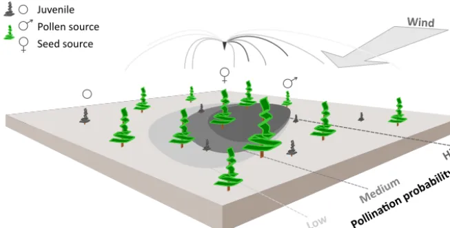
Pollen was not represented in the former LAVESI version, but is needed to independently track gene flow by seeds and pollen through time. Accordingly, Figure 1 illustrates how we implemented an individual based pollination for each seed’s ovule using a wind-determined and distance-dependent probability distribution function for pollen disper-sal (similar to Gregory, 1961). It makes use of the von Mises distribution, which is an angular equivalent to the Gaussian normal distribution, for the two-dimensional representation (Abramowitz and Stegun, 2012).
A pollen dispersal function was newly implemented as a distance-dependent probability function for pollination of each individual seed’s ovule, rather than simulating the large amount of pollen released by each tree (Gregory, 1961; Ku-parinen et al., 2007). For each seed-bearing tree, the proba-bility of pollen donating trees is calculated and out of the list of potential fathers for each seed one tree is randomly de-termined according to this probability. The pollination prob-ability of each seed’s ovule on a tree is proportional to the amount of pollen in the air column around it, which is, for simplification in the current implementation, not additionally dependent on the performance of the tree so that every tree that bears cones is taken into account. This aspect might be included in future versions. The following function is used here as the distance-dependent probability distribution of ar-riving pollen:
pr=exp
−2per1−0.5m
√
π C (1−0.5m)
, (1)
whereris the distance in m,peis the ratio of pollen
descend-ing velocityVd, pollenestimated forLarix gmelinii(Eisenhut,
1961) and wind speedVwand Gregory’s parametersC and mare set toC=0.6 cm−(1−0.5m) andm=1.25 (p. 167 in Gregory, 1961).
The probability distributionprdescribed in Eq. (1) is
mul-tiplied by the von Mises distribution (Eq. 2), a continuous probability distribution on the circle, to include pollen dis-tribution over a certain area and couple the process to the wind direction (illustration in Fig. 1; Abramowitz and Ste-gun, 2012).
pv=
exp κcos θ−θ
2π I0(κ) , (2)
whereκ is the inverse of the von Mises distribution’s vari-ance, andI0(κ)is the modified Bessel function of order 0 as
Wind
Juvenile Pollen source Seed source
Pollina
�on pr
obabili ty
Low
Mediu
m
High
Figure 1. Schematic representation of wind pollination as newly implemented in the LAVESI-WIND model. Based on actual winds, a
distance-dependent pollination probability of ovules is estimated for each adult tree (potential pollen source) and for each seed source in the simulated area. The shaded areas on the ground represent the pollination probability for the labelled seed source for winds from the upper-right corner. These are generally higher for adult trees in upwind direction of the central seed source.
Consequently, following Gregory (1961) the pollination probability of a seed’s ovule is as follows:
p=prpv=exp
−2p
er1−0.5m
√
π C (1−0.5m)
exp κcos θ−θ
2π I0(κ) .
(3) 2.2.2 Seed dispersal
In the initial version of LAVESI, seeds are dispersed in ran-dom directions and at a distancerin m, estimated by a Gaus-sian and negative exponential (fat-tailed) dispersal function (Eq. 5, Kruse et al., 2016):
r=
r
2E02(−log(rand))+1
2distance ratio·rand
−1.5, (4)
whereE0, originally named “width”, is the Gaussian
distri-bution’s standard deviation in m, “rand” stands for a random number∈ [0,1]and “distance ratio” is a weighing factor for the fat tail in m2. Parameter estimates were based on a sen-sitivity analysis in Kruse et al. (2016) and numerical experi-ments.
The wind-dependent distance estimation was implemented as a ballistic flight following the assumptions of Mat-lack (1987). Accordingly, seed dispersal distances depend on the height of the releasing tree top Ht in m, currently esti-mated as 75 % ofHt(factorfHt =0.75), and are modified by
wind speedVWin m s−1and a species-specific fall speed of propagules (seed plus wing)Vd=0.86 m s−1forL. gmelinii:
E0=fHt·Ht·
VW
Vd
. (5)
Finally, the direction for the seed dispersal is determined by wind direction, which was randomly selected from a set of observations (see Sect. 2.2.5 for details).
2.2.3 Parameterization to fit field data
The model’s parameters had to be revised after implement-ing the model extensions to achieve simulated tree densities comparable to field data. Forest inventory data were recorded for each larch individual with explicit positions on plots of a minimum area of 20×20 m for several locations along a den-sity gradient from single-tree stands in the north to dense for-est tundra stands in the south visited on summer expeditions in the years 2011 and 2013 in northern central Siberia, Rus-sia (Wieczorek et al., 2017). We conducted simulations on 100×100 m areas with closed boundaries initialized by intro-ducing 1000 seeds in the first 100 years of a stabilization pe-riod of 1000 years, with forcing climate data randomly sam-pled from the available data. For the final 80 years of each simulation we used the climate series from the correspond-ing field site (TY04, see Sect. 2.2.4 for details). We visually compared the number of trees at year 2011 from the central 20×20 m area to the field survey data, which was the first year of fieldwork. The parameters were manually tuned and we iteratively performed simulation runs to improve the sim-ulation results until finally achieving similar stand densities (numbers of trees) as observed (data not shown; parameter values in Table 1).
2.2.4 Temperature and precipitation
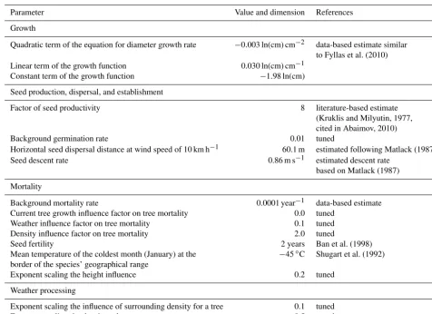
re-Table 1.Overview of model parameters and processes forL. gmeliniiindividuals that are different from the original version (Kruse et al., 2016).
Parameter Value and dimension References
Growth
Quadratic term of the equation for diameter growth rate −0.003 ln(cm) cm−2 data-based estimate similar
to Fyllas et al. (2010)
Linear term of the growth function 0.030 ln(cm) cm−1
Constant term of the growth function −1.98 ln(cm)
Seed production, dispersal, and establishment
Factor of seed productivity 8 literature-based estimate
(Kruklis and Milyutin, 1977, cited in Abaimov, 2010)
Background germination rate 0.01 tuned
Horizontal seed dispersal distance at wind speed of 10 km h−1 60.1 m estimated following Matlack (1987)
Seed descent rate 0.86 m s−1 estimated descent rate
based on Matlack (1987)
Mortality
Background mortality rate 0.0001 year−1 data-based estimate
Current tree growth influence factor on tree mortality 0.0 tuned
Weather influence factor on tree mortality 0.1 tuned
Density influence factor on tree mortality 2.0 tuned
Seed fertility 2 years Ban et al. (1998)
Mean temperature of the coldest month (January) at the −45◦C Shugart et al. (1992)
border of the species’ geographical range
Exponent scaling the height influence 0.2 tuned
Weather processing
Exponent scaling the influence of surrounding density for a tree 0.1 tuned
Exponent scaling the density value 0.5 tuned
sponses and derive the auxiliary climate variables active air temperature (sum of temperatures above 10◦C, AAT10) and vegetation length (number of days exceeding the freezing point, net degree days, NDD0) to calculate tree growth, esti-mate individual tree mortality and establishment from seeds (details in Kruse et al., 2016). We selected a grid box in-tersecting a location with a known northern taiga tree stand (CH06 at 70.66◦N; 97.71◦E, site CF in Wieczorek et al., 2017) and a northern forest tundra stand (TY04, 72.41◦N; 105.45◦E, site FTe in Wieczorek et al., 2017). From the available data we excluded years before 1934, because of missing climate station data and hence unreliable extrapo-lations in the data set (Mitchell et al., 2004). Furthermore, the final year was set to 2013, which is the latest year of fieldwork. The climate at these sites either allows strong tree growth with mean July temperatures of 13.50◦C, cold-est temperatures during January of −33.24◦C and a pre-cipitation sum of∼328 mm year−1or only sparse stands to emerge with temperatures of 13.11 and −36.07◦C in July and January, respectively, and ∼247 mm annual precipita-tion (cf. Kruse et al., 2016).
2.2.5 Wind speed and direction
The model is driven with pairs of wind speed in m s−1 and wind direction in degrees [◦]. The winds at 10 m above the surface for the years 1979–2012 at 6-hourly resolution were extracted from the ERA-Interim reanalysis data set (Fig. 3; Balsamo et al., 2015). Because of the coarse spatial resolu-tion (80×80 km), we considered only the grid box over the climate station Khatanga, which is situated roughly in the centre of the treeline ecotone on the southern Taymyr Penin-sula (71.9◦N; 102.5◦E; Wieczorek et al., 2017). During sim-ulation runs, values are randomly drawn from the year’s veg-etation period (May–August; Abaimov, 2010) for each seed dispersal event and for the determination of pollination. For simulated years in which climate data are available but no corresponding wind data, a year is randomly selected. 2.3 Sensitivity analyses for dispersal processes
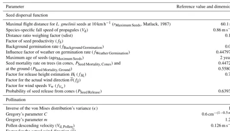
Rails-Table 2.Parameter values evaluated in the sensitivity analysis for seed dispersal, migration patterns, and pollination.
Parameter Reference value and dimension
Seed dispersal function
Maximal flight distance forL. gmeliniiseeds at 10 km h−1(rMaximum Seeds, Matlack, 1987) 60.1 m
Species-specific fall speed of propagules (Vd) 0.86 m s−1
Distance ratio weighing factor (sdist) 0.16
Factor of seed productivity (fS) 8
Background germination rate (fBackground Germination) 0.01
Influence factor of weather on germination rate (fWeather Germination) 0.447975
Maximum age of seeds (ageMaximum Seeds) 2 years
Seed mortality rate on trees (in cones,PSeed Mortality, Cones)and 0.44724
at the ground (PSeed Mortality, Ground) 0.55803
Factor for release height estimationHt(fHt) 0.75
Factor for the actual wind directionθ(fθ) 1
Factor for wind speedsVw(fVw) 1
Probability of seed release from cones (PSeed Release) 0.63931
Pollination
Inverse of the von Mises distribution’s variance (κ) 10
Gregory’s parameterC 0.6 cm−(1−0.5m)
Gregory’s parameterm 1.25
Pollen descending velocity (Vd, Pollen) 0.126 m s−1
Factor for the actual wind direction (θ ) 1
back, 2005; Cariboni et al., 2007). For each simulation re-peat, the input parameters (Table 2) were changed by 5 % and 50 % and a sensitivity value was calculated by comparing the results with the reference run:
S+/−=
V+/−−VREF
VREF
P+/−−PREF
PREF
, (6)
whereV is the variable of interest derived from each simu-lation run andP is the parameter of interest, both plus (+) and minus (−) 5 % of the estimated parameter, or with the reference value (Kruse et al., 2016).
The simulations were carried out on hypothetical north– south transects with a width of 100 m and length of 1000 m using the new model version and allowing seeds to be dis-persed along the meridional borders. Populations were ini-tiated on empty areas only in the lowermost 100 m wide and 100 m long area by randomly distributing 1000 seeds during the first 10 years of a 1000 year long stabilization period. During this phase, seeds exceeding the lowermost 100×100 m area were removed from the simulation. In the following simulation period seeds could enter the area above 100 m and colonize this empty area. The simulation model randomly drew weather conditions for each year from the complete available period 1934–2013 during the stabi-lization and simulation period. These simulations were re-peated 30 times and the positions of each individual tree were recorded at the end of the simulation (500 years). To directly compare results from simulations with changed parameters
to reference runs the simulation period was repeated for each parameter variation starting with an identical state of the sim-ulation at the end of the stabilization period and using the same climate series.
For the evaluation of migration rates we selected three tar-get output variables for the area ahead of the 100 m initial-ization area: (1)stemcountis the total number of stems (trees with a height above 130 cm), (2) forested area is the area covered with >100 stems ha−1, and (3)peak recruit posi-tionis the position of the maximum number of stems on the basis of a running mean with a 50 m window. Additionally, the variablestand density, which is the number of stems in the 20×20 m plot in the centre of the lowermost area, was selected to assess impacts on plot level. Furthermore, the
pol-lination distanceexpressed as the mean distance between the
pollen-donating and seed-producing trees was calculated for the evaluation of the pollination function. The resulting sen-sitivity values were tested for significant changes from the reference results (mean of 0) with at test with a confidence level of 95 %.
2.4 Model-performance experiments
processes to estimate the total memory needed for the arrays of trees and seeds and the grid representing the environment (Kruse et al., 2016).
To reduce the computation time, we parallelized the code for estimating pollination probabilities, seed dispersal, and tree density computation of the model using the OMP-library and conducted simulations using 1, 4, 8, and 16 CPUs. The performance of the model was evaluated by recording the computation time of each single simulation year for com-plete simulation runs (1080 years). We conducted four dif-ferent runs, one with only wind dispersal of seeds (SEED), one with seed and pollination (+POLL), and two different parallelized pollination computations. First, we tried to sim-ply compute equally sized parts of the complete list of tree individuals including trees that have not produced seeds on the selected number of CPUs (+POLL_PAR-A). In a sec-ond variant (+POLL_PAR-B), we attempted to decrease the potential computational overheads of idle CPUs that had fin-ished their job faster because of fewer individuals that needed to estimate pollination for produced seed’s ovules, by cut-ting the list to only trees that produce seeds. The compu-tation time increases with the actual number of trees and seeds present in simulations. In consequence, we analysed the dependency between the time needed for each simulated year and the number of trees and, additionally, the number of produced seeds by generalized nonparametric regression (us-ing the “gam”-function in R-package “gam”; Hastie, 2017). The dependent variable timet was log-transformed prior to analysis. The explanatory variables – number of treesNtand seedsNs– were parametrically fitted and tested for non-linearity by comparing the deviance of a model that fits the terms linearly with a chi-squared test. In the initial model for-mula, we also included the interaction between the explana-tory variables and excluded non-significant terms from the linear model (p >0.05) until yielding the final best model.
3 Results
3.1 Verification of wind-dependency
The simulated seeds were solely dispersed in a north or south direction in coherence to the forcing winds (Fig. 2, Tables S2 and S3). The median seed dispersal distances were∼12.2 m with a north wind and ∼12.0 m with a south wind with a majority of 95 % falling within∼43 m of the seed tree, but with rare (∼0.1 %) dispersal events>1000 m (Fig. 2). The distance is equally highly correlated with the release height for both wind directions (ρ=0.63,p <0.0001; Fig. 2).
The pollination events were mainly coming from the di-rection of the forcing winds: however,∼18 % deviated from the forcing wind direction (Table S4). This variance is intro-duced by the formulae used for calculating the pollination probability for each seed’s ovules on a tree and is further in-creased by the random selection of a father out of a subset
Release height [cm]
Seed dispersal distance [m]
100 200 500 1000
0.1
10
1000
10
0
00
0
10
0
00
00
0
● Simulated
Simulated median Expected median 1 and 99 % 25 and 75 % CI
Figure 2.Dispersal distances of seeds are wind dependent and
pos-itively correlated with the height of the releasing tree. The simu-lated and hypothetically calcusimu-lated dispersals were compared across evenly distributed height classes; the results are similar for north and south winds, and here the results with north winds are pre-sented.
of all possible mature trees based on the probability density function. The median distance along forcing winds of∼38 m is, in general, shorter by∼3–5 m than in other directions (Ta-ble S4).
In northern central Siberia, the main wind directions ob-served during the vegetation period are a combination of both west and east (Fig. 3a). In some years, one of these di-rections predominates, and is also characterized by stronger wind events. Accordingly, simulated seeds are dispersed into the general direction of the forcing wind data (Fig. 3b). Dis-persal distances can reach up to a maximum of several thou-sand kilometres, yet the majority of seeds fall within a few hundreds of metres, and these are dispersed over distances depicting the wind speeds as well.
The median pollen flight distances are generally larger than the seed’s, with a technically fixed maximum of about the distance from the central plot to the borders (Fig. 3c). Similar to seed dispersal, pollination follows the wind direc-tions and fathers are positioned in the upwind direction of the main occurring winds.
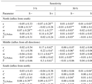
3.2 Sensitivity analyses for implemented dispersal processes
1979–2012 1990 1998
(a) Wind speeds
(b) Seeding
(c) Pollination
W
S N
E 5 %
10 % 15 % 20 % 2 5% 30 % %
W
S N
E 5 %
10 % 15 % 20 % 25 % 30 % 35%
W
S N
E 5 %
10 % 15 % 20 % 25 % 30 % 35%
[m s−1] 0 to 2 2 to 4 4 to 6 6 to 8 8 to 10 10 to 17.102
W
S N
E 5 %
10 % 15 % 20 % 25%
W
S N
E 5 %
10 % 15 % 20 % 25% 30%
W
S N
E 5 %
10 % 15 % 20 % 25% 30%
[m] 0 to 50 50 to 100 100 to 150 150 to 200
W
S N
E 5 %
10 % 15 % 20 % 25 % %
W
S N
E 5 %
10 % 15 % 20 % 25 % 30% 35%
W
S N
E 5 %
10 % 15 % 20 % 25 % 30% 35%
[m] 0 to 5 5 to 10 10 to 25 25 to 50 50 to 100 100 to 200 200 to 6.3406e+06
Figure 3.Wind forcing(a), simulated seed dispersal(b), and pollination distances(c)by distance and cardinal direction. Simulations were
performed on 200×200 m plots and seed dispersal events tracked away from source trees: pollination events were recorded from pollen
donor trees standing in the plot area into the central 20×20 m plot.
more apparent becomes the change in the result so that the significance increases strongly from only 25 % to 79 %. The sensitivity values were of the same order of magnitude with the extreme values of −1.89 and 3.26 for each per-cent change in the input parameter. Most sensitive is the position of the peak recruitment for the observed migration rate (mean absolute sensitivity of 1.09 and 0.92 for 5 % and 50 %), whereas the impact on the stand level is of minor im-portance (with sensitivities of only 0.28 and 0.19). The factor of seed productivityfSand the influence factor of weather on germination ratefWeather Germinationled to strongest advances
of thepeak recruit positionif increased, which the seed mor-tality rate on treesPSeed Mortality, Conescaused when lowered.