Annales Geophysicae (2001) 19: 229–244 © European Geophysical Society 2001
Annales
Geophysicae
Ozone isotopic composition: an angular effect
in scattering processes?
F. Robert1and C. Camy-Peyret2
1CNRS-Mus´eum, Laboratoire de Min´eralogie, 61 rue Buffon, 75005 Paris, France
2CNRS-Laboratoire de Physique mol´eculaire et applications, Universit´e Pierre et Marie Curie, Tour 13, Bte 76 - 4 place Jussieu, 75252 Paris Cedex 05, France
Received: 19 June 2000 – Revised: 5 December 2000 – Accepted: 11 December 2000
Abstract. The ratio of the differential scattering cross
sec-tions involving distinguishable and indistinguishable isotopes may exhibit non-mass dependent angular variations. A nu-merical application of this hypotheses to the ozone reaction rates reproduces some of the results observed in laboratory experiments. This theory could be tested through a cross beam experiment where the isotopic composition of the scat-tered products is recorded as a function of their scattering angles.
Key words. Atmospheric composition and structure (middle
atmosphere – composition and chemistry)
Glossary
General formalism
– A and B: two isotopes of the same chemical element – XA and XB: two isotopically substituted molecules – [A] and [XA]: the number densities of A and XA, respec-tively
– R as subscript: stands for reactive. Used for reactions yielding an exchange of isotopes such as A+XB→ XA+
B
–NR as subscript: stands for non-reactive. Used for reac-tions which do not yield an isotope exchange such as A+
XB→A+XB
–T as subscript: stands for total
–kA−XB,R: isotopic exchange rate constant –α: isotopic fractionation factor
–θandπ−θ: the scattering angle expressed in coordinates of the center of mass frame (see Figs. 1 and 3)
–θXA: the scattering angle of XA
–F (θ ): the differential cross section describing the particle scattering at a collisional angleθ and at relative velocityv. Usually reported in the literature asF (θ )= |f (θ )|2
–8i: in the cross beam experiments, the flux of speciesi Correspondence to: F. Robert ([email protected])
–xi: the relative isotopic abundance of isotopei P xi =1 –β(θ )=1/2{FT(θ )+FT(π−θ )}/FT(θ )
–2: the range of scattering angles,2= [θ1, θ2]
–k(2): the rate constant for reactions between distinguish-able isotopes for a given distribution of speeds and angles; notedhF (θ, v)iin the text
k(2)= Z ∞
0
vf (v)dv Z θ2
θ1
[FNR(θ, v)+FR(θ, v)]sinθ dθ – ki(2): the rate constant for reactions between indistin-guishable isotopes for a given distribution of speeds and an-gles: 1/2{FT(θ )+FT(π−θ )}in place ofFNR(θ )+FR(θ ) ink(2)
–β(2)=ki(2)/ k(2) General relations
–FNR(θ )+FR(θ )=FT(θ )
–FNR(π−θ )+FR(π−θ )=FT(π−θ ) –G(θ )=1/2{FT(θ )+FT(π−θ )}
– If2= [0, π], k(2)=ki(2), β(2)=1 Ozone formalism
–16O,17O and18O: the three isotopes of oxygen
– [O2], [O], [M], [O∗3]: the number densities of molecular O2, atomic O, the third body M and of activated complex, respectively
–k∗: the rate constant for the formation of the activated com-plex O∗
3
–kD(2): the rate constant for the spontaneous dissociation of the activated complex, in a scattering domain of angles 2, resulting from interactions involving distinguishable iso-topes
–ki,D(2): the rate constant for the spontaneous dissociation of the activated complex, in a scattering domain of angles2, resulting from interactions involving indistinguishable iso-topes
230 F. Robert and C. Camy-Peyret: Ozone isotopic composition
1 Introduction
The first measurement of mass independent oxygen isotopic fractionation was reported by Clayton et al (1973) in the high temperature minerals of carbonaceous meteorites. In 1980 Cicerone and McCrumb (1980) reported an 18O en-richment in atmospheric ozone. Mauersberger (1981, 1987) measured enrichments in the18O/16O ratio of stratospheric ozone relative to that of atmospheric oxygen, and came to the decisive conclusion according to which such an enrich-ment cannot be explained by the standard theory of isotope fractionation. Krankowsky et al. (2000) have shown that stratospheric ozone exhibits an isotopic fractionation in per-fect agreement with laboratory determinations but somewhat lower than those measured in 1981. A crucial step in under-standing this effect was made by Thiemens and Heidenreich (1983) and Heidenreich and Thiemens (1986) who demon-strated that the isotope distribution in ozone was non-mass dependent, i.e. that the relative isotopic fractionation for 17O/16O was equal to that for18O/16O. Such a relation be-tween the two oxygen isotopic ratios was in disagreement with all known isotope fractionation mechanisms. Indeed, all these mechanisms yield a mass dependent isotope frac-tionation, i.e. a relative variation in the17O/16O ratio of 1% should be accompanied by a 2% variation in the18O/16O ratio. Clearly the theory developed by Urey (1947) and Bigeleisen (1947) for isotope fractionation in thermodynam-ical equilibrium and in kinetic processes, respectively, does not predict these isotope effects (see also Kaye and Strobel, 1983; Kaye, 1986).
Additional measurements in natural ozone by Mauersber-ger (1987), Abbas et al. (1987), Goldman et al. (1989), Goldman et al. (1998), Schueler et al. (1990) have con-firmed the mass independent isotopic fractionation in ozone, although these analyses showed large differences in the iso-topic fractionation factor. Numerous laboratory studies using mass spectrometry (Morton et al., 1989; Morton et al., 1990; Thiemens and Jackson, 1987; Thiemens and Jackson, 1990; Yang and Epstein, 1987), diode laser technique (Anderson et al., 1985) and infrared absorption (Bahou et al., 1997) have shown enrichment in the heavy isotopomers of ozone.
Several attempts to reconcile the isotope fractionation the-ory with these observations have been made. For example, a proposal of Valentini (1987) involved nonadiabatic tran-sitions from5 or1 molecular electronic states to6 elec-tronic states. This explanation was rejected by Morton et al. (1989) based on detailed laboratory studies where the excited electronic states did not contribute to the synthesis of ozone. Bates (1988) argued against these explanations and suggests that the lifetime of symmetrical and unsymmet-rical activated complexes are different because of the lack of randomization of their internal energies. Recently, Gel-lene (1996) proposed a model of symmetry-induced kinetic isotope effects. According to this model, when a homonu-clear diatomic molecule is involved in the O+O2reaction, only a fraction of the rotational states correlate with those in the ozone molecule, yielding a depression of the rate
con-stant of this reaction relative to those involving heteronuclear molecules. But this explanation is in conflict with recent experimental results (Mauersberger et al., 1999). Although the physical reason for these anomalies remains unknown, it has been suggested that a mechanism involving a modifica-tion of the classical recombinaison theory (Anderson et al., 1985; Bates, 1988; Heidenrich and Thiemens, 1986; Gellene, 1996) or the formation of electronically excited ozone (An-derson et al., 1992; An(An-derson and Mauersberger, 1995) dur-ing the O+O2collisions was necessary (see also the recent reviews by Thiemens (1999) and Mauersberger et al. (1999), in the introduction of their 1999 article).
In the present paper we will follow another approach pro-posed by Robert et al. (1988) and Robert and Baudon (1990) in which there is no need for consideration of symmetry of the O2or O3molecules. Contrary to the previous approaches, we will show that a specific aspect of isotopic reactions has been omitted in the theoretical treatment of isotopic fraction-ation. In the usual theory it is assumed that no difference (beside the usual mass difference between isotopes) can ex-ist between the scattering cross sections of the different iso-topes of the same element, because the interaction potential of isotopic species is essentially the same. In fact, a marked difference does exist between the collision cross sections in-volving distinguishable and indistinguishable isotopes. This effect remains a “classical” effect. We will show that sev-eral laboratory data can be reproduced numerically if one as-sume that this difference is at the origin of the isotope effects observed during the synthesis of ozone. To emphasize this point, we have purposely ignored other isotope effects (Se-hested et al., 1995; Anderson et al., 1997; Bahou et al., 1997) which have been shown to contribute to the overall ozone iso-topic fractionation.
Therefore, throughout the paper we will consider that the three isotopes of oxygen have the same mass, i.e. can be distinguished essentially by their “names”: 16, 17 and 18. By neglecting the mass difference, we will put into focus the marked differences in the behavior of isotopes considered now as individual particles (distinguishable or not), with no reference to the type of chemical bound they are involved into. Using this unique assumption we will show that some of the experimentally observed isotopic fractionation can be numerically reproduced within the framework of the classi-cal model for ozone reaction rates. The validity of the present approach remains to be tested by a more rigorous quantum mechanical calculation (which is not the purpose of this pa-per).
2 General formulation for atom-diatom isotopic exchange
2.1 Preliminary remarks
iso-F. Robert and C. Camy-Peyret: Ozone isotopic composition 231 topes of the same element. This approximation permits
sev-eral simplifications in the formalism developed in the fol-lowing, but will not be repeated when it applies. It should be kept in mind that no isotopic fractionation is expected within this assumption because all known isotope effects depends ultimately upon this mass difference which determines the internal energy differences between the isotopically substi-tuted molecules. It is also important to understand that within this assumption all the isotopic cross sections for isotopically substituted molecules are strictly equal.
2.2 Mass dependent isotopic fractionation in equilibrium and in kinetic processes
2.2.1 Thermodynamic equilibrium
The rate of a bimolecular isotope exchange reaction
A+XB−−−−−−→kA−XB,R B+XA (1)
is generally considered as a weighted mean contribution of rates of individual process for all the internal states (reac-tants and products). In Eq. (1)kstands for the rate constant and the subscriptR(R stands for reactive) indicates that an isotopic exchange takes place in the course of the reaction A+XB. For simplicity, the dependence with temperature (usually notedk(T )in the literature) is omitted in our no-tation. A reaction rate similar to (1) can be written for B involved in the reverse reaction
B+XA−−−−−−→kB−XA,R A+XB. (2)
By definition the isotopic fractionation factor is
α=kA−XB,R/ kB−XA,R. (3)
Since the differences in the isotopic masses are neglected, α = 1 in (3) indicates that no isotope fractionation is ex-pected under thermodynamic equilibrium. At equilibrium for an isolated system involving only reactions (1) and (2), the isotopic abundances are related by the relation
α=([B]/[A]) / ([XB]/[XA]) . (4) Introducing the masses of the reactants in Eq. (3), yields the common isotope fractionation effect for whichαis slight-ly different from unity because of small differences in the internal states of the different isotopic molecules.
2.2.2 Kinetic processes
In kinetic processes the isotopic fractionation is supposed to take place between the activated complex (noted∗) and the reactants. Such a process is illustrated by the following reac-tions:
A+XB
kA−XB∗ ,R
−−−−−−→AX. . .B∗, (5)
A+XB
kA−XB∗ ,NR
−−−−−−−→A. . .XB∗, (6)
A+XA
kA−XA∗ ,T
−−−−−−→A. . .X. . .A∗. (7)
An exchange of isotopes may (reaction 5) or may not (re-action 6) take place during the re(re-action between A and XB (subscriptNRfor the non-reactive reaction). The total rate constant (subscriptT) is used to describe reaction (7) involv-ing identical isotopes(A+XA)because it is impossible to decide if an isotopic exchange took place or not during the reaction. This total rate constant is always supposed to be the sum of the reactive and the non-reactive processes k∗A−XA,T =kA−XA∗ ,R+k∗A−XA,NR. (8) In a mixture of A, B, XA and XB, the rate of disappearance of A occurring via the formation of the activated complex can be written
−d[A]/dt=kA−XB∗ ,R[A][XB] +k∗A−XB,NR[A][XB] (9)
+kA−XA∗ ,T[A][XA].
A similar equation can be written for−d[B]/dt. The ratio of the disappearance rates is then
(−d[A]/−d[B])/([A]/[B])= {kA−XB∗ ,T[XB] (10)
+kA−XA∗ ,T[XA]}/{kB−XA∗ ,T[XA] +kB−XB∗ ,T[XB]}. Since in our idealized system, the isotopic masses are ne-glected
k∗B−XA,T =kB−XB∗ ,T =kA−XB∗ ,T =k∗A−XA,T (11) and Eq. (10) becomes
{(−d[A]/−d[B])/([A]/[B])} =1. (12) Equation (12) indicates that no isotopic fractionation takes place during the formation of the activated complex. Intro-ducing the isotopic masses in (10) yields the usual isotopic fractionation effect for which
{(−d[A]/−d[B])/([A]/[B])} 6=1. (13) Therefore, mass effects yield, both in equilibrium and in kinetic processes, the so called “mass dependent fractiona-tion effect” (see “introducfractiona-tion” for this definifractiona-tion). Such an effect is not considered in the present paper.
2.3 Possible origin of the mass independent isotope effect The isotopic effect we wish to describe here is entirely caused by reactions involving indistinguishable isotopes (such A+
XA). More specifically, it is linked to a difference in the distribution in space of the products of reactions involving distinguishable and indistinguishable isotopic species.
Consider the distribution in space of the products when the reactants are isotopically distinguishable. Such a situ-ation can be illustrated by the encounter of a beam of XA molecules with a beam of B atoms:
XA
−−→←−B
232 F. Robert and C. Camy-Peyret: Ozone isotopic composition Figure 1 : F. Robert & C. Camy-Peyret in Ozone isotopic composition
NON REACTIVE Figure 1a
XA
XA
B
B θ θ XA
θ B
DA, up
DB, down
REACTIVE Figure 1b
XA
A
B
XB
θ θA
θ XB
dΩ dt dΩ dt ΦXAΦΒ FNR(θ)
d[B] d[XA] Φ
XAΦΒ FNR(θ) = = =
dΩ dt dΩ dt
ΦXAΦΒ FR(θ)
d[XB] d[A] Φ
XAΦΒ FR(θ) = = =
=θ
=θ
=θ
=θ
DA, up
DB, down
Fig. 1. Schematic diagram of the trajectory of different isotopic species as a function of their scattering angles in a cross beam ex-periment between XA and B. A and B are two isotopes of the same element. “Reactive” indicates that isotopes are exchanged in the course of the collision. A and XA are detected byDAand B and XB byDB. The differential scattering cross section measured by
DAandDBare strictly equal atθXA=θB=θ.
(1) The angles of the collisionθXAandθB(see Fig. 1a), defined in the co-ordinates of the center of mass of the atom molecule system, are expressed relative to the directions of the isotopes A or B in the beams before the collision. For simplicity, scattering is described only for the two spatial dimensions; azimutal angles are not introduced in the for-malism. Since we are only interested in reactions between isotopes, the spectator atom X plays no role and its possible collision with B is not considered.
(2) Two detectors notedDAandDBin Fig. 1 (in opposite direction in the center of mass reference), measure the flux of the scattered species; DA records A and XA while DB records B and XB. In principle, the atom A and the molecule XA can be distinguished by the detectorDA and similarly forDB. This classical experiment allows the determination of the differential scattering cross sections, i.e. the variations of the fluxes of A or XA as a function ofθAorθXA, and the variations of the fluxes of B or XB as a function ofθBorθXB. We noteF (θ )the differential cross section as a function of the scattering angleθ(see glossary for definition).
XA B
XA
,
NR
A,
RXB,
Rπ
π
/ 20
F
(
θ
)
B,
NRXB/A
XA
/B
(
θ
)
(
θ
)
(
θ
)
up
down
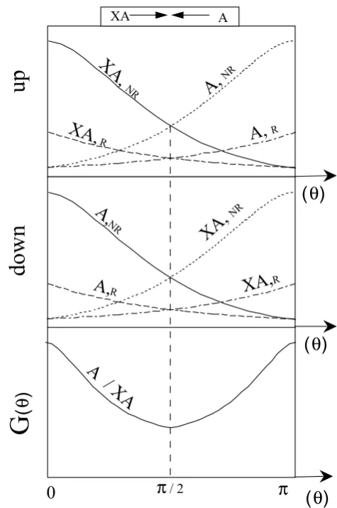
Fig. 2. Schematic diagram of the isotopic distributions of XA, XB, A and B, as a function of their scattering angles in the cross beam experiment shown in Fig. 1. The probability for detecting XA and B atθXA=θB=θare strictly equal (and similarly for XB and A). The reactive and non-reactive overall differential cross sections are reported in the lower part of the figure.
(3) As shown in Fig. 1, two reactions can occur and the products of these reactions detected byDAandDBare XA+B→XA(atθXAinDA,NR)
+B(atθBinDB,NR) Fig.1a (14) XA+B→XB(atθXBinDB,R)
+A(atθAinDA,R) Fig.1b (15) As for cross sections, NR and R stand for non-reactive and reactive reactions, respectively. In such an experiment the two products of the same encounter are detected “simul-taneously”, since if we are to get a molecule in the positionθ there must be an atom in the opposite side at the angleπ−θ. Therefore, the distributions as a function ofθfor atoms and molecules resulting from the same reaction are strictly equal.
(4) We note8ithe flux of speciesi.
[image:4.595.304.543.63.427.2]F. Robert and C. Camy-Peyret: Ozone isotopic composition 233
XA
XA
θ A
θ XA
REACTIVE
A
A
DA(up)
DA (down)
A
XA
XA
A
NON REACTIVE DA(up)
DA (down)
REACTIVE
XA
A
XA
A DA(up)
DA (down)
XA
XA
A
A
NON REACTIVE
θ θ XA
DA(up)
DA (down) θ
θ
θ
=θ
θ A=θ
=θ =θ
π−θ
A
θ =
π−θ
XA
θ =
π−θ
A
θ =
π−θ
XA
θ =
π−θ
A
θ =
[image:5.595.303.541.61.419.2]Figure 3a
Figure 3b
Figure 3c
Figure 3d
Fig. 3. Schematic diagram of the trajectory of different isotopic species as a function of their scattering angles in a cross beam ex-periment between XA and A. A and XA are detected by the upper and lower detectorsDA. As for the reactions between XA and B, the differential scattering cross sections measured by the upper and lower detectorsDAare strictly equal.
these two reactions, for a given initial relative velocity, are d[XA]/ddt=d[B]/ddt=8XA8BFNR(θ ) , (16) d[XB]/ddt =d[A]/ddt=8XA8BFR(θ ) . (17) In such a situationFNR(θ )andFR(θ )are clearly differ-ent since they correspond to differdiffer-ent pairs of molecule/atom products, i.e. XA/B and XB/A, scattered in opposite direc-tions. Schematic diagrams ofF (θ )for atoms and molecules scattered in space by the two reactions (14) and (15) are re-ported in Fig. 2.
One could also introduce in the theory the “impact param-eter” to describe the distribution in space of the products of the collisions. This impact parameter is omitted here because it is entirely dictated by the relative velocityvand the scat-tering angle, which are the explicit parameters of the cross sections we will use hereafter.
Consider now the same experiment with A in place of B: XA
−−→←−A
Figure 4 : F. Robert & C. Camy-Peyret in Ozone isotopic composition
XA A
XA
,
NRXA,
RA,
NRA,
Rup
A,
NRA,
RA /
X
A
π
π
/ 20
XA
,
NR
XA,
R(
θ
)
(
θ
)
G
(
θ
)
(
θ
)
up
down
Fig. 4. Schematic diagram of the isotopic distributions of XA and A as a function of their scattering angles in the cross beam experi-ment shown in Fig. 3. Although drawn for heuristic purposes, XA and A resulting from reactive and non-reactive reactions cannot be experimentally distinguished. “Reactive” indicates that isotopes are exchanged in the course of the collision. The resulting overall dif-ferential cross sectionG(θ )=1/2{FT(θ )+FT(π−θ )}describing the reactions between A and XA is drawn in the lower part of the figure.G(θ )exhibits a marked enhancement aroundθ=πas com-pared toF (θ )(see Fig. 2).
In such a case, two reactions which were not detectable in the previous experiment, can now be detected by the two de-tectorsDA. These reactions are shown in Fig. 3. These two reactions are the reactive and non-reactive reactions at the scattering angleπ−θ. To ease the discussion, let us desig-nate arbitrarilyDA(up)andDA(down)the upper and lower detectors in Fig. 3, since these two detectors can always be experimentally distinguished. The following reactions will be detected:
XA+A→XA(θXAinDA,NR(up))
+A(θAinDA,NR(down)) Fig.3a (18) XA+A→XA(θXAinDA,R(down))
234 F. Robert and C. Camy-Peyret: Ozone isotopic composition XA+A→XA(θXAinDA,NR(down))
+A(θAinDA,NR(up)) Fig.3c (20) XA+A→XA(θXAinDA,R(up))
+A(θAinDA,R(down)) Fig.3d (21) When a species A (and similarly for XA) is detected at any angle it is impossible to tell if the individual scattering process was reactive or non-reactive (see Figs. 3b, c). This is different from the same individual process for distinguish-able isotopes for which there is no ambiguity to asses that a reactive collision occurred if A is detected. Schematic dia-grams of the functionsF (θ )for atoms and molecules scat-tered in space by these four reactions are reported in Fig. 4. At this stage, we have therefore reached the central (and unique) assumption of the paper: the total cross section must be used to describe the reaction A+XA. This assumption is illustrated in the lower part of the Fig. 4 where the cross sec-tions for the reacsec-tions A−XA are constructed using exactly the same rules defined for the reactions between A and XB.
The differential number of molecules or atoms scattered by these four reactions are
d[XA]/ddt=d[A]/ddt =8XA8A1/2{FNR(θ ) +FNR(π−θ )+FR(θ )+FR(π−θ )}. (22) SinceFNR(θ )+FR(θ )=FT(θ )
d[XA]/ddt=d[A]/ddt
=8XA8A1/2{FT(θ )+FT(π−θ )} =8XA8AG(θ ).(23) The factor 1/2 is introduced in (22) since we have to con-sider four possible reactions between XA and A and only two between XA and B. This factor 1/2 is also introduced in classical mechanics to prevent a double counting when the particles are identical.
Using these results, it is possible to predict the isotopic composition of atoms and molecules as a function of their scattering angle in the following idealized experiment:
XA,XB
−−−−−→←−−−A,B
The following reactions should take place: A+XA→A+XA
1/2{FT(θ )+FT(π−θ )} =G(θ ) (24) B+XB→B+XB
1/2{FT(θ )+FT(π−θ )} =G(θ ) (25)
A+XB→A+XB FNR(θ ) (26)
A+XB→B+XA FR(θ ) (27)
B+XA→B+XA FNR(θ ) (28)
B+XA→A+XB FR(θ ) (29)
The corresponding cross sections are indicated for each reac-tions. According to our formalism the molecular products of
Figure 5 : F. Robert & C. Camy-Peyret in Ozone isotopic composition
(
θ
)
π
π
/ 20
θ
1θ
2F
R(
θ
)
F
NR(
θ
)
G(
θ
)
F
T(
θ
)
Θ
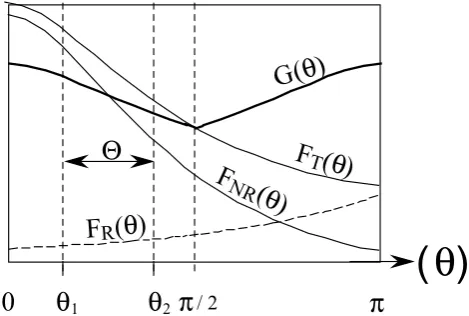
Fig. 5. Schematic differential cross sections forFNR(θ ), FR(θ ),
FT(θ )=FNR(θ )+FR(θ )andG(θ )=1/2{FT(θ )+FT(π−θ )}.
F functions stand for distinguishable isotopic reactions andGfor undistinguishable. The domain2= [θ1, θ2]marks the domain of angle where the activated complex cannot possibly stabilize. Since
G(θ )6=FT(θ ), an isotopic fractionation as a function of the scat-tering angle is expected.
these reactions at the same angleθ=θXA =θXBare d[XA]/ddt =8XA8BFNR(θ )+8XB8AFR(θ )
+8XA8A1/2{FT(θ )+FT(π−θ )}, (30) d[XB]/ddt =8XB8AFNR(θ )+8XA8BFR(θ )
+8XB8B1/2{FT(θ )+FT(π−θ )}. (31) Let us assume for simplicity that there is no isotopic frac-tionation between the beams
8XA8B=8XB8A. (32)
Then, the production rate ratiod[XA]/d[XB]is (d[XA]/d[XB])/(8XA/8XB)
= {xB+xAβ(θ )}/{xA+xBβ(θ )} (33) with
β(θ )=1/2{FT(θ )+FT(π−θ )}/FT(θ )
=G(θ )/FT(θ ) (34)
and withxAandxBthe relative abundance of the isotopes A and B
xA+xB=1 (35)
for a chemical element having two isotopes.
In quantum mechanics,β(θ )can be6=1 becauseFT(θ )is not symmetrical aroundπ/2 (as shown from the individual FR(θ )andFNR(θ )in Fig. 2). Therefore,G(θ )is markedly different fromFT(θ )and an isotopic fractionation is expected as a function of the scattering angle, i.e.
[image:6.595.308.543.64.222.2]F. Robert and C. Camy-Peyret: Ozone isotopic composition 235
G(θ )andFT(θ )are compared in Fig. 5. Note that in clas-sical mechanics, as for example in the case of the scattering of rigid spheres,FT(θ )does not vary withθand Eq. (34) is equal to unity, i.e. no isotopic fractionation is expected as a function of the scattering angleθ.
The theoretical result of Eq. (33) can be tested in a cross beam experiment where the isotopic compositions of the scat-tered species are measured as a function of their scattering angles.
Suppose that these isotopic reactions take place in a real mixture and are followed by a chemical reaction whose prod-ucts are selected according to the scattering angles of the iso-topic species (i.e. according to their internal energy after the reaction). In such an angular selection, the fraction of the reactants which return to the initial mixture can be described by the following reaction
A+XB−−−→k(2) A+XB (or B+XA) . (37) 2designates the domain of scattering angles lying between θ1 andθ2 (see Fig. 5) where A and XB are not stabilized in the form of a new chemical species(2 = [θ1, θ2]). An isotope exchange may or may not occur during the reaction; hence the notation “or B+XA”.
In Fig. 5, it can be observed that in the forward scatter-ing interval2 = [0, θ1],G(θ ) < FT(θ ) whereas in most of the backward scattering interval 2 = [θ2, π], one has G(θ ) > FT(θ ). This illustrates the fact that, depending on the considered system, i.e. depending on the width and po-sition of2, isotopic enhancement is scattering angle depen-dent.
The corresponding rate constantk(2)describing the iso-topic composition of atoms and molecules that return to the mixture is the result of averagingFT(θ, v)over the appropri-ate distribution of speeds and angles
k(2)= hFT(θ, v)i (see glossary for definitions). (38) In such conditionsβ(2)can be defined as
β(2)=ki(2)/ k(2) (39)
with
ki(2)= hG(θ, v)i. (40)
k(2)andki(2) stand for the rate constants involving dis-tinguishable and indisdis-tinguishable isotopes, respectively. We will show in the next section that, ifβ(2)is known, the iso-topic composition of these atoms and molecules can be cal-culated. Note also that, if the integration is performed over all the scattering angles(2= [0, π]), no isotopic fractiona-tion is expected and, as in classical mechanics
β(2)=1. (41)
From (33) it can be seen that this type of isotopic frac-tionation will rely entirely on the relative isotopic abundance
of a chemical element and thus, can be defined as an “abun-dance dependent” isotopic fractionation. It should be noted that the isotope effect resulting from (34) is in accordance with the Pauli exclusion principle according to which it is not “permitted” to separate in the calculation, the cross sec-tion describing the incident from the recoil particle, if the two particles are indistinguishable.
3 Theoretical application to ozone formation
3.1 Reaction rate model
In order to simplify the formalism, the classical model for the formation rate of ozone will be used. The mass independent isotopic fractionation expected from the theory developed in the preceding section will be used within the framework of this model.
This model is derived from the three following reactions:
O+O2→O∗3 k∗ (42)
O∗3→O+O2 kD(2) (43)
O∗3+M→O3+M kM (44)
Equation (42) describes the formation of the activated com-plex O∗3with the rate constantk∗. Equation (43) represents the spontaneous dissociation of the complex with the rate constant kD(2) (D for dissociation); its inverse 1/ kD(2) characterizes the lifetime of the complex. In the present treat-ment we assume that the dissociation of the complex is pos-sible only in a scattering angle domain 2 (see the defini-tion of2in the glossary); hence the notationkD(2). Equa-tion (44) corresponds to the possible stabilizaEqua-tion of O∗
3by a third body M bringing out the proper amount of internal energy. The overall formation rate of ozone is derived as-suming that the concentration of the activated complex O∗3is constant (steady state), that is
d[O∗3]/dt=0. (45)
Under this condition we have
k∗[O][O2] −kD(2)[O∗3] −kM[O∗3][M] =0 (46) and the production rate of O3is
d[O3]/dt= [O∗3][M]kM. (47)
From Eqs. (46) and (47), the rate of the overall reaction
O+O2+M→O∗3+M (48)
can be derived
d[O3]/dt= [O2][O]{k∗kM[M]/(kD(2)+kM[M])}. (49) In the case of the “low pressure approximation”kM[M] kD(2)
236 F. Robert and C. Camy-Peyret: Ozone isotopic composition The usual three body recombinaison rate is recovered in this
case as kMO+O
2 =k ∗
kM/ kD(2) (51)
and the value recommended by DeMore et al. (1997) will be used for the numerical applications
kMO+O
2(300 K)
=(6.0±0.5)·10−34cm6molecule−2s−1 (52) with the following temperature dependence
kMO+O
2(T )=k M
O+O2(300 K) ·
300 K T
2.3±0.5
cm6molecule−2s−1. (53) In the case of the “high pressure approximation”kM[M] kD(2)and
d[O3]/dt = [O2][O]k∗. (54)
3.2 Formalism for isotopic reactions
In this section we write the general rules for the reactions involving all the possible isotopic substitutions in O3. In order to reduce the number of possible reactions, the three isotopes of oxygen (16O,17O,18O) are designated by A, B and C. With this notation, the entire system can be described by four types of reactions: A+AA, A+AB, A+BC and A+BB. As compared to the previous discussion on isotopic exchanges involving A+XB or A+XA, we now consider that X can be A, B or C. For simplicity in the forthcoming re-actions, the third body M will be omitted in the reactions of complex stabilization; hence the use of the notationkM[M].
The goal of the following paragraphs is to provide a ba-sis for calculating the appropriate formation rated[ABC]/dt of the various isotopomers of O3 using equations similar to (49).
3.2.1 Reaction between indistinguishable isotopes (1) A+AA:
A+AA k
∗
−→AAA∗ (55)
AAA∗−−−−−→ki,D(2) A+AA (56)
AAA∗−−−−→kM[M] AAA (57)
This reaction involves only indistinguishable isotopes. In this case we designate the decomposition rate byki,D(2). (2) A+AB:
A+AB 1/2yk ∗
−−−−−→AAB∗ (58)
AAB∗−−−−−→ki,D(2) A+AB (59)
AAB∗−−−−→kM[M] AAB (60)
The factor 1/2 in (58) indicates that the probability of hav-ing a collision with A is exactly equal to the probability of having the same collision with B in the heteronuclear mole-cule AB. Each reaction of A with one of the two atoms of AB is thus counted separately and bold italic is used in this discussion to designate the knock-on atom. In our notations we designate the middle atom as the apex of the isosceles tri-angle which is the normal equilibrium configuration of ozone in its ground electronic state.
The factoryis introduced here because it is assumed that the activated complex has only two channels to be rearranged into its stable form
AAB∗→AAB, (61)
AAB∗→ABA. (62)
The incident atom can be (1) either attached to the knock-on atom of the molecule (with a branching ratioy) (2) ei-ther attached to the spectator atom of the molecule (with a branching ratio 1−y) or (3) inserted between the knock-on and the spectator atom. We neglect this third possibility (see Bahou et al., 1997, for the experimental determination of this contribution). Thus, the other stabilizing channel is
A+AB 1/2(1−y)k ∗
−−−−−−−−−→ABA∗, (63)
ABA∗−−−−−→ki,D(2) A+AB, (64)
ABA∗−−−−→kM[M] ABA. (65)
There are only two possible rearrangements of the complex and thus
yk∗+(1−y)k∗=k∗. (66)
3.2.2 Reaction between distinguishable isotopes (1) A+BA:
A+BA 1/2yk ∗
−−−−−→ABA∗ (67)
ABA∗−−−−→kD(2) A+BA(or B+AA) (68) ABA∗−−−−→kM[M] ABA(orBAA via(1−y)k∗) (69) Exchange and non-exchange processes are not counted sep-arately in (68) since they do not cause any isotopic fraction-ation between the activated complex and the reactants be-side usual mass dependent effects; hence, the notation “or B+AA”.
(2) A+BC: A+BC 1/2yk
∗
−−−−−→ABC∗ (70)
F. Robert and C. Camy-Peyret: Ozone isotopic composition 237
(3) A+BB: A+BB 1/2k
∗
−−−−→ABB∗ (73)
ABB∗−−−−→kD(2) A+BB(or B+AB) (74) ABB∗−−−−→kM[M] ABB(orBBA) (75) In this case the two isotopomers are the same (ABB and
BBA); hence, the branching ratioyis not appearing. 3.3 Interpretation of the formalism for isotopic reactions All the rules defined by Eqs. (55) to (75) are based on a single idea: the ozone isotopic composition is entirely gov-erned by a statistical distribution of isotopes between the re-actants. We simply assume that the decomposition of the activated complex is not possible at all angles and therefore, that its decomposition rate cannot be counted similarly if its formation involves distinguishable or indistinguishable iso-topes. In the following we discuss the physical significance of the four constantsk∗,ki,D(2),kD(2)andkM[M]. 3.3.1 The constantk∗
For all the reactions, we consider that the activated molecules are formed by all the possible collisions between atoms and molecules, occurring at all angles. There is no need to dis-criminate the rate constants for the formation of the activated complex by reactions involving distinguishable and indis-tinguishable isotopes; hence, the use of the same constant k∗, for the formation of all activated complexes. Such an equality implies that the isotopic composition of the activated complex is not fractionated relative to the isotopic composi-tions of atoms and molecules, besides usual mass dependent effects.
3.3.2 The relation betweenki,D(2)andkD(2)
We then consider that among all the possible angles at which the activated complex could dissociate, there is only a small fraction of them where it is stabilized via its subsequent re-actions with M (see Fig. 5). Therefore, in this model, atoms and molecules that return to the gas do not result from all the scattering angles.
It is possible to relate theki,D(2)/ kD(2) ratio with the β(2)factor defined in the previous section. Assuming
d[O∗3]/dt=0 (76)
we can write the relations between distinguishable and in-distinguishable processes. For this purpose we compare, as an example, the reactions between16O and17O18O (i.e. in-volving only distinguishable species) and between16O and 16O16O (involving only indistinguishable species)
[16O][17O18O]hFT(θ, v)i = [16O17O18O∗]kD(2) , (77) [16O][16O16O]1/2hFT(θ, v)+FT(π−θ, v)i
= [16O16O16O∗]ki,D(2) . (78)
Since we assume that no isotopic fractionation took place between the reactants and the activated complex O∗
3
[16O17O18O∗]/[16O16O16O∗]
= [16O][17O18O]/[16O][16O16O]. (79) The relation betweenki,D(2)/ kD(2) can then be derived through the ratio (78)/(77)
ki,D(2)/ kD(2)=1/2hFT(θ, v)+FT(π−θ, v)i
/hFT(θ , v)i =β(2) . (80)
This formalism will be used hereafter for numerical simula-tions of the different ozone isotopomer production rates of reactions (57) to (75). From (80) it should not be concluded that, contrary to a previous suggestion by Bates (1988), the life time of the activated complex16O16O16O∗ is different from that of16O17O18O∗. As for cross sections, this reflects the fact that it is not possible to distinguish between activated complexes resulting from16O16O+16O collisions at scatter-ing anglesθfrom those atπ−θ. The numerical values of β(2)are estimated in Sect. 4.2.
3.3.3 The constantkM
No isotopic fractionation is supposed to take place during the stabilization of the complex, and thuskMis the same for all the isotopically substituted species.
3.4 Formalism for isotopic reaction rates
The partial formation rate of any particular isotopomer (from AAA of reaction (55) to ABB of reaction (75)), can be cal-culated using (49) with the proper identification of 1/2k∗, kD(2),ki,D(2)andkM[M]in place ofk∗,kD(2)andkM[M] appearing in the original Eq. (49). The calculation was per-formed using the following parameters:
K=kD(2)/ kM[M], (81)
C=(β(2)K+1)/(K+1) . (82)
With the rules defined from (55) to (75), the ratio of the iso-topic reaction rates can be calculated
d[16O16O17O]/d[16O16O16O]
=1/2(1+C)[16O][16O17O] +C[17O][16O16O]
[16O][16O16O] (83)
and similarly with18O in place of17O in Eq. (83). In the same manner we have
d[16O17O17O]/d[16O16O16O]
=1/2(1+C)[17O][16O17O] +C[16O][17O17O] [16O][16O16O] (84) and similarly with18O in place of17O in Eq. (84). Finally, for the fully mixed isotopomers, we have
d[16O17O18O]/d[16O16O16O]
=C [16O][17O18O] + [17O][16O18O]
238 F. Robert and C. Camy-Peyret: Ozone isotopic composition The density of the isotopic species [O] and [O2] are
calcu-lated statistically
[iO] = [O]xi (86)
[iOjO] = [O2]2xixj (87)
withxi andxj the relative abundance ofiO andjO, respec-tively withP
xi =1. In the next calculation we assume that the gas can be considered as an infinite reservoir relative to ozone, i.e. that the isotopic composition of molecular oxygen remains constant through time.
As far as the parameteryis concerned, it dictates only the final configuration of the ozone molecule. When the isotopic composition of ozone is determined mass spectrometrically, the different isotopomers of ozone (as for example, BAC and ACB) cannot be distinguished and there is no need of tak-ing into account the parameter y. However, in one of the reported laboratory experiments discussed hereafter, the po-sition of the atoms in ozone was determined by Anderson et al. (1989) by infrared spectrometry and related to the iso-topic fractionation. Other observations of the symmetrical and non-symmetrical isotopomers of ozone were obtained in the stratosphere by infrared spectroscopy (Goldman et al., 1989). As we will see in the numerical applications, exper-imental results show thaty ≈0.1, indicating that the prob-ability of the incoming atom to be attached to the spectator atom of the molecule is close to unity. Thus, and contrary to other proposed models, the symmetry of the O3molecule does not play any special role in the present model.
4 Application to observed isotopic fractionation in ozone
In this section we compare the numerical predictions of the present theory with the observed isotopic fractionation in well defined laboratory systems. For practical purpose a set of for-mula with the numerical values of the parameters are given in the Appendix. The proper identification of the terms can be derived from Sects. 2 and 3. Numerous experimental papers have been published on the subject of isotopic enhancements in O3 and we have selected several types of results which represent the most typical and puzzling aspects of this mass independent isotopic fractionation.
4.1 Data basis
We will numerically address the following observations: (1) The isotopic variations in17O/16O and18O/16O with pressure reported by Thiemens and Jackson (1990). This experiment reproduces two unique features of this mass in-dependent fractionation: (i) contrary to the classical predic-tions, the fractionation varies with pressure and (ii) almost identical relative variations are observed for both the17O/16O and18O/16O ratios. On the contrary, the “classical” theory of isotopic fractionation predicts a linear correlation with slope 1/2 between the relative variations of the two isotopic ratios. (2) The plateau in the isotopic fractionation factor observed at low pressure by Morton et al. (1990). This result suggests
that the isotopic fractionation factor becomes constant below ca. 100 Torr.
(3) The distribution in the mass range 48 to 54 amu. of ozone isotopic species. This distribution is markedly dif-ferent from that expected from the classical mass-dependent isotope fractionation theory (Morton et al., 1989; Mauers-berger et al., 1993) or from simple statistical distribution of isotopes among O3. Recently, Sehested et al. (1998) and Mauersberger et al. (1999) reported the rate constants for the different reactions O+O2involving all the possible permu-tations between16O,17O and18O. These rates will be com-pared with the present calculations and will be propagated to the isotopomers of ozone for comparison with the recent data from Wolf et al. (2000).
(4) The asymmetrical ozone molecule16O16O18O which carried more than twice the isotopic enrichment of the sym-metrical ozone molecule16O18O16O (Anderson et al., 1989). Similar observations were performed by Christensen et al. (1996), Larsen et al. (2000) and Janssen et al. (1999) for both16O16O18O and16O18O18O. These observations are im-portant since in the present theory the isotopic fractionation is independent of the symmetry of the ozone molecule.
We will show that all these results are a possible conse-quence of the isotopic indistinguishibility.
4.2 Estimation of theβparameter
In the next sections (4.3 to 4.6)β(2)is considered as a free parameter and its value is adjusted in order to reproduce the measured isotopic fractionation in ozone. It is nevertheless possible to estimate to what extentβ(θ )of (34), i.e. before averaging over 2, can be different from unity, i.e. differ-ent from the “transmission coefficidiffer-ent” which is taken to be equal to 1 in the usual kinetic isotopic fractionation theory (cf. Bigeleisen, 1947). Two limiting cases can be distin-guished:
(1) forθaround 0,FT(θ )FT(π−θ ); thusβ(θ )=1/2, (2) forθaroundπ,FT(π−θ )FT(θ ); thusβ(θ )1.
F. Robert and C. Camy-Peyret: Ozone isotopic composition 239 4.3 Isotopic fractionation with pressure
Mass spectrometric experimental data are from Thiemens and Jackson (1990) and Morton et al. (1990). We have selected the photolysis experiments where ozone was produced in pure O2. In these experiments no attempt was made by the au-thors to identify the ozone isotopic species carrying the iso-topic anomaly and the17O/16O and18O/16O isotopic ratios represents the bulk value of the mixture of all isotopically substituted ozone molecules.
Since the position of18O in heavy ozone is irrelevant for mass spectrometry measurements we do not introduce in the calculation the branching ratioy (see Sect. 3.2). In order to be more realistic we have introduced in the calculation two mass-dependent isotopic relations fork∗andβvalues. They are introduced as
k∗l−mn=k∗(µl−mn/µ16−1616)a. (88) µis the reduced mass for O−O2,l,mandnstand for mass 16, 17 or 18, l stands for atoms, mn for molecules. The parametera is usually taken equal to−1/2 or−1/3. This gives the usual mass-dependent relationship
k17−1616∗ =k∗(1+εk) and k18−1616∗ ∼=k∗(1+2εk) . (89) εdesignates the isotopic fractionation factor expressed per mass unit. The same treatment was applied forβ (hence the notationεβ). The isotopic composition of ozone in a given experiment is expressed in the usualδunits
δiO(‰)= [(iO/16O)experiment/(iO/16O)statistic−1] ×1000 (90) Such a treatment allows the calculation of the slope s de-fined by the linear relation betweenδ17O(‰) andδ18O(‰) in the three isotope diagram: s = 1(δ17O)/1(δ18O). For the mass-dependent isotopic fractionation(β =1), the slope sis calculated with the present theory to vary between 0.514 and 0.529 forδ17O varying between+50‰ and−50‰, re-spectively. These numerical results are in excellent agree-ment with values measured by several authors (Clayton et al. 1973; Robert et al., 1992; Meier and Li, 1998).
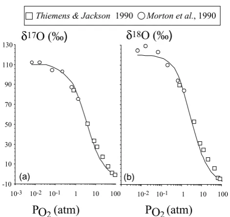
The calculations of the isotopic composition of ozone as a function of pressure are reported in Figs. 6a, b. They were performed by adjusting the model parameters to the ex-perimental results. That iskD(2)/ kM = 1020,β = 1.15, εk = −10‰,εβ = +32‰. The variation with pressure of the parameterK (K =kD(2)/ kM[M]) was calculated rig-orously, i.e. using the proper equation of state for gaseous molecular oxygen to determine [M] as a function of the pres-surePO2. It should be noted that the final isotopic compo-sition of ozone depends strongly on the actual value of β while the three other parameters do not affect this isotopic composition by more than a few per mil. Taking a numeri-cal example of such relations between parameters, a change from 1.15 to 1.16 in theβ value yields roughly an isotopic effect of 10‰.
Figure 6 : F. Robert & C. Camy-Peyret in Ozone isotopic composition
-10 10 30 50 70 90 110 130
1 10 100
10-3 10-2 10-1 10-2 10-1 1 10 100
δ
17O (‰)
δ
18O (‰)
Thiemens& Jackson 1990 Morton et al., 1990
(a) (b)
[image:11.595.307.543.59.281.2]P (atm)
O
2P (atm)
O
2Fig. 6. Calculated variations (solid lines) of (a)δ17O(‰) and (b)
δ18O(‰) as a function of pressure. Experimental data are from Thiemens and Jackson (1990) and Morton et al. (1990).
At a first order of approximation, the value of the ratio kD(2)/ kM = 1020 molecule cm−3 which fits the isotopic variations as a function of pressure, is consistent with the pre-vious estimates published in the literature. In the notations of Kaufman and Kelso (1967),kD(2)/ kM is notedkb/ kc with kb=3·1010s−1andkc=1·10−11cm3molecule−1s−1 pre-ferred by these authors to those of Klein and Herron (1966), i.e.kb=1.8·109s−1andkc=7·10−13cm3molecule−1s−1. The corresponding values ofkb/ kcare 3·1021and 2.6·1021, respectively. Althoughkbandkcvary by more than one or-der of magnitude, these authors choose the same value forka (k∗ in our notation, i.e. k∗kD(2)/ kM = kakb/ kc) yielding identicalkb/ kcratios. Considering the whole range of vari-ations ofkbandkcmeasured by these authors, akb/ kcratio ranging between 1.8·1020and 4·1022seems possible, hence compatible with 1·1020calculated here.
At a second order of approximation an interesting effect may be related to the difference between kD(2)/ kM and kb/ kc. As proposed by Pack et al. (1998), several types of activated complexes seem to exist in three body reactions. It could then be admitted that the activated complex, involved in the angular isotopic effect described here, has ak∗value different from that determined through the low pressure ap-proximation (see Eq. 50).
240 F. Robert and C. Camy-Peyret: Ozone isotopic composition
250
-50 0 50 100 150 200
49 51 53
Mass Number
50 52 54
48
Enrichment (‰)
Morton et al., 1989
Present calculation
Fig. 7. Calculated enhancements in the different isotopically substi-tuted ozone molecules (from17O16O16O to18O18O18O; mass 49 to 54) are compared with experimental data (Morton et al., 1989).
low and high pressure were performed by different labora-tories. Since they are reproduced numerically for the same value of the parameters, these parameters are used for all the following calculations.
4.4 Non mass-dependent fractionation in ozone isotopomers
Morton et al. (1989) and Mauersberger et al. (1993) recorded the isotopic fractionation linked to the isotopic substitution in O3. These data are compared in Fig. 7 with the theo-retical predictions of the present model using the previously determined parameters forβ, εk, εβ and K. The isotopic abundances and the pressure correspond to the experimen-tal conditions indicated by Morton et al. (1989) in their pa-per. As observed in Fig. 7 the marked enhancement in the 16O17O18O/16O16O16O ratio (at mass 51 in the figure) rel-ative to the other isotopically substituted species is qualita-tively reproduced by the calculation, as well as the interme-diate enhancement at masses 49, 50 , 52 and 53. However, the theoretical pattern is systematically lower than the exper-imental data. This can be understood as follows.
In the experiment reported by Morton et al. (1989), ozone was formed by an electric discharge while the different pa-rametersβk,εk,εβ andKwere determined in Sect. 4.3 for ozone produced by photolysis (Thiemens and Jackson, 1990; Morton et al., 1990). Therefore, it is conceivable that the pa-rameterβ is also linked to different experimental techniques to generate ozone. For example, ifβis adjusted to 1.17
(in-Table 1. Comparison between observed and calculated isotopic fractionation in ozone isotopomer (expressed in per mil) produced by photolysis. Data are from Mauersberger et al. (1993). The pa-rameters of the calculation are defined in Sect. 4.3. Papa-rameters:
β = 1.15, a = −0.25, b = 0.80,c = 0,P = 100 Torr; see appendix
Enrichment (‰)
Mass Species Observed Calculated Difference
48 16O16O16O ≡0 ≡0
49 16O16O17O 113 109 −4
50 16O17O17O 121 110 −11 50 16O16O18O 130 118 −12
51 16O17O18O 181 186 +5
51 17O17O17O −18 −15 +3 52 16O18O18O 144 120 −24
52 17O17O18O 95 129 +34
53 17O18O18O 83 130 +47
[image:12.595.51.283.61.324.2]54 18O18O18O −46 −29 +17
Table 2. Comparison between the rate constants measured by Sehested et al. (1998) with the calculations using the parame-ters given in Sect. 4.3. 16O+16O16O (k1), 18O+16O16O (k2) and16O+18O18O (k3),16O+16O18O (k4) and18O+16O18O (k5), 18O+18O18O (k
6)
Sehested et al. (1998) Present calculation
(k2+k3)/2k1 1.184±0.037 1.185
(k4+k5)/2k1 1.155±0.062 1.086
k6/ k1 0.977±0.021 0.977
stead of 1.15 used here), the calculated enhancements for all the species translate upward and match almost exactly the mass 49, 50, 51 and 52.
A similar experiment has been repeated by Mauersberger et al. (1993) for photolysis experiments and the isobaric in-terferences at mass 50, 51 and 52 were estimated. These experimental results are reported in Table 1 and compared with our theoretical calculations using the previously deter-mined β, εk, εβ and K parameters. This comparison re-veals several encouraging points: (1) the theoretical and ob-served isotopic fractionation for the mass dependent frac-tionated species 17O17O17O and 18O18O18O are in agree-ment within±15‰, (2) the theoretical and the observed iso-topic fractionation for the anomalously fractionated species at mass 49 to 51 are in agreement within±8‰, (3) at higher masses, and especially for the two species17O17O18O and 17O18O18O, the experimental isotopic fractionation is about 35‰ lower than calculated. This point will be addressed in Sect. 4.5. However, according to our calculation, these ef-fects contribute at most for 30% of the net effect.
[image:12.595.311.543.402.454.2]F. Robert and C. Camy-Peyret: Ozone isotopic composition 241
Figure 8 : F. Robert & C. Camy-Peyret in Ozone isotopic composition
1.00
0.80 0.90 1.10 1.20 1.30 1.40 1.50 1.60
[image:13.595.58.280.93.300.2]10.5 11.0 11.5 12.0
Reduced Mass lO - [mOnO]
Isotopomer Rate Coefficients (rel. to 16O16O16O)
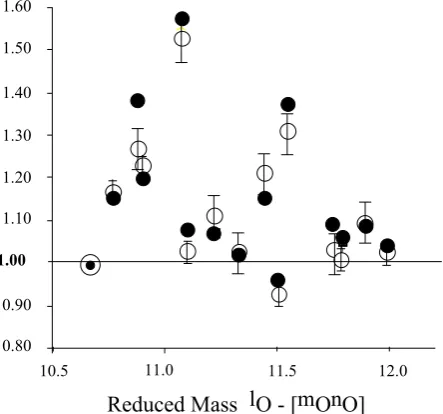
Fig. 8. Specific rates coefficients for isotopomer as a function of the reduced mass for the reactionslO+mOnO (l,mandnstand for mass 16, 17 or 18). Data (open disks) from Mauersberger et al. (1999) are shown with their error bars and calculated values are in black. The calculation is performed in the low pressure approxi-mation witha = +0.3,b = −3.5,c = +10 andβ = 1.20; see appendix.
for the reactions16O+16O16O(k1),18O+16O16O(k2)and 16O+18O18O(k
3), 16O+16O18O(k4)and18O+16O18O (k5), 18O+18O18O (k6). For these reactions, the results of our calculated rate constants are reported in Table 2 and compared with those of Sehested et al. The calculations are in perfect agreement for the reactions involving only distin-guishable isotopes (i.e.18O+16O16O and16O+18O18O) or only indistinguishable isotopes (i.e. 18O+18O18O). How-ever for the reactions involving one distinguishable and one indistinguishable isotopes (i.e. 16O+16O18O and18O
+16O18O), the calculated rate constants are in slight dis-agreement with observations (1.086 and 1.155±0.062 re-spectively). Note that the experimental result is also in agree-ment with the reactions rates measured or derived by Mauers-berger et al. (1999). We will see in the next section that the disagreement is caused by the reaction16O+16O18O whose calculated rate is 1.19 while its measured rate is 1.27. This may be caused by an additional isotopic effect of the sym-metrical relative to the asymsym-metrical variant of the molecule which is not modeled in the present theory.
4.5 Isotopomer specific rate coefficients
Contrary to the first order of approximation used in Sects. 4.3 and 4.4 according to which the value ofβ is equal for all types of reactions between O and O2, the results obtained by Mauersberger et al. (1999) put into light another
prop-Table 3. Isotopomer specific rate coefficients calculated with the parameters defined in the appendix and having the valuesβ=1.22,
a=0.3,b= −3.4,c=10,P =0 Torr. Measured rates are from Mauersberger et al. (1999)
Reactions Calculated Measured Reduced
Rate Rate Mass
16O+16O16O ≡1 ≡1 10.67 17O+16O16O 1.08 1.03 11.10 18O+16O16O 0.96 0.93 11.52 16O+17O17O 1.39 1.23 10.88 17O+17O17O 1.02 1.02 11.33 18O+17O17O 1.10 1.03 11.77 16O+18O18O 1.58 1.53 11.08 17O+18O18O 1.39 1.31 11.55 18O+18O18O 1.04 1.03 12.00 16O+16O17O 1.15 1.17 10.78 17O+16O17O 1.08 1.11 11.22 18O+16O17O 1.03 nd 11.65 16O+16O18O 1.20 1.27 10.88 17O+16O18O 1.23 nd 11.33 18O+16O18O 1.06 1.01 11.77 16O+17O18O 1.49 nd 10.98 17O+17O18O 1.16 1.21 11.44 18O+17O18O 1.10 1.09 11.89
erty ofβ: its value is also mass-dependently related with the mass of the molecule involved in the isotopic reaction. As for reaction (88), this relation can be written as
βmn−16 =β(µ16−mn/µ16−1616)c. (91) This dependence is different from that illustrated by reaction (88) describing the relation ofβwith the reduced mass of the reactants. As a whole,βcan be written
βmn−l =β(µ16−mn/µ16−1616)c(µl−mn/µ16−1616)b (92) (as in (88) l, m, n designates 16, 17 ,18 and l stands for atoms andmnfor molecules). Therefore, in this theory, the only non classical (i.e. non mass-dependent) parameter is β, i.e. the rate constant ratio describing the reactions be-tween distinguishable and undistinguishable isotopes. The mass-dependent parametersa,b, andcwere adjusted to the following values: a = +0.3, b = −3.4 and c = +10, corresponding to 15‰/amu,−130‰/amu and+105‰/amu, respectively. Numerical results are reported in Table 3 for β = 1.22 and reproduce within±3% the data reported by Mauersberger et al. (1999). These results are also reported in Fig. 8 as a function of the reduced mass of the reactants for the individual rateslO+mOnO.
[image:13.595.327.530.125.366.2]242 F. Robert and C. Camy-Peyret: Ozone isotopic composition
Table 4. Comparison between calculations performed for isotopi-cally non-fractionated (column 1) and fractionated (column 2) oxy-gen atoms in a scrambled gas. The calculations were performed at 60 Torr with the parameters reproducing the isotopomer specific rate coefficients (Mauersberger et al., 1999; cf. Table 3). Recent data at 60 Torr on all ozone isotopomers are reported for compari-son (Wolf et al., 2000). The difference between the results in col-umn 2 and the measured isotopic composition are reported in the last column (1)
Enrichment (‰)
Mass Species Column 1 Column 2 Measured 1
Calculated Calculated
48 16O16O16O ≡0 ≡0 ≡0 ≡0
49 16O16O17O 129 114 106 8
50 16O17O17O 188 159 110 49 50 16O16O18O 121 96 130 −34
51 16O17O18O 248 206 198 8
51 17O17O17O 18 −22 −15 −7 52 16O18O18O 234 180 161 19 52 17O17O18O 142 83 94 −11
53 17O18O18O 195 121 89 32
54 18O18O18O 36 −43 −39 −4
with this calculation. In two cases, an individual rate (cf. Table 3) is directly comparable with the isotopic composi-tion of an isotopomer obtained in scrambled mixtures: this is the case for 18O18O18O (and similarly for 17O17O17O) which can result from only one reaction, i.e.18O+18O18O. The measured reaction rate in pure18O for18O+18O18O is
+30‰ (i.e. 1.03 in Table 4) while in scrambled mixtures the isotopomer18O18O18O is fractionated by≈ −40‰ (cor-responding to 0.96), i.e. by−70‰ relative to the predicted value of+30‰. As suggested by Mauersberger in reviewing the present article, isotope exchange reactions are fast and, under equilibrium, the18O/16O atomic oxygen ratio should be 76‰ relative to the statistical composition of the mixture (Anderson et al., 1997). Such an isotopic fractionation of atoms has been introduced in the present calculations and was mass-dependently propagated for all the reactions con-tributing to the formation of all the isotopomers. This effect can also be reproduced within the framework of the present theory by replacing the parametera =0.30 in Eq. (88) by a = −0.36. Results are reported in Table 4 and compared with the results expected without taking into account this ef-fect.
From Table 4, it can be verified that, taking into account the isotopic fractionation of oxygen atoms in the gas, the-oretical and experimental results become closer. On av-erage, the absolute differences between the calculated and the measured δ18O values of the different isotopomers are within±20‰. However they are not statistically distributed around zero. For example, the differences are still large for 16O16O18O (−34‰),16O17O17O (+49‰) and17O18O18O
Table 5. Exit channel specific rate coefficients for the formation of 50O
3and52O3. The parameters of the calculations are defined in appendix and determined from specific rates coefficients (see Table 3): β = 1.2,a = 0.3, b = −3.5,c = 10,P = 0 Torr. The probability for an incoming atom to be attached to the knock-on atom of the O2molecule is designated byy. Measured ratios are from Janssen et al. (1999)
Reactions Calculated Ratio Measured
y=0.5 y=0.1 Ratio 16O+16O18O→16O16O18O 1.19 1.33 1.45±0.04 16O+18O16O→16O18O16O 1.19 1.04 1.08±0.01 18O+16O16O→18O16O16O 0.94 0.94 0.92±0.04 18O+16O16O→16O18O16O 0.0 0.0 0.006±0.005 18O+18O16O→18O18O16O 1.05 1.06 0.92±0.06 18O+16O18O→18O16O18O 1.05 1.03 1.04±0.02 16O+18O18O→16O18O18O 1.55 1.55 1.50±0.03 16O+18O18O→18O16O18O 0.0 0.0 0.029±0.006
(+32‰) (cf. Table 4; remember that symmetrical and un-symmetrical variants are not separated in mass spectrome-try) while, for other species, they are smaller than 20‰. This departure between theoretical and experimental enrichments is not statistically different from what was obtained for cal-culated individual rates and, in this respect, likely represents the highest degree of approximation which can be reached by the present theory.
4.6 Isotopomer fractionation ratio
Anderson et al. (1989) reported the ratioR1= [16O16O18O]/
[16O18O16O]which ranges from 2.27 to 2.19 according to the highest and lowest isotopic enrichment levels, respec-tively, that could be achieved in their experiment (ozone be-ing produced by electric discharge). Larsen et al. (2000) have reported the determination of the ratioR2 = [16O18O18O]/
[18O16O18O]along withR1: within the uncertainties of the measurements,R1cannot be distinguished from its classical value of 2.0, whileR2lies between 2.42 and 2.52. Janssen et al. (1999) reported the four possible rates yielding to 16O16O18O and16O18O16O along with the four possible rates yielding to16O18O18O and18O16O18O. The corresponding R1 andR2(R1 = 2.75 andR2 = 2.33) are different from Anderson et al. (1989) and also different from Larsen et al. (2000).
[image:14.595.310.545.159.282.2] [image:14.595.52.285.181.341.2]F. Robert and C. Camy-Peyret: Ozone isotopic composition 243 the parametery, i.e. the probability for an incoming atom
to be attached to the knock-on atom of the O2molecule (see Eq. 58). In Table 5, calculations are reported fory = 1/2 andy =0.1. Fory =0.1 the numerical results are in close agreement with the determinations of Janssen et al. (1999).
Note that the departure ofR1 from its classical value of 2 is entirely due to the reaction between indistinguishable isotopes. If this reaction is ignored (i.e. ifβ = 1, b = 0, c=0) the ratio of the two isotopomers is exactly 2.00±0.03 whatever the values of all the other parameters.
4.7 Isotopic fractionation with temperature
Morton et al. (1990) have reported the isotopic fractiona-tion of ozone as a funcfractiona-tion of temperature. The variafractiona-tion with temperature of the rate constants involved in the for-mation of ozone has been established in the literature (see DeMore et al., 1997). Introducing these numerical results in the present theory (see Eq. 53) does not yield the results obtained by Morton et al. (1990) for the isotopic fraction-ation. This may indicate that the parameterβ also depends on the temperature. If this interpretation is correct, such a relation betweenβ and the temperature can be understood as follows: the scattering angles at which ozone is stabilized vary with temperature, i.e. with the internal energy at which the activated complex is formed. No attempt was made here to take into account this dependence.
5 Conclusions
Hathorn and Marcus (1999) have proposed another interpre-tation of the oxygen isotope effect in ozone based on the fact that the asymmetric ozone isotopomers have a larger density of reactive states compared with that for symmetric species. Therefore, the role played by the molecular symmetry in this isotopic effect should be used to test these two theories.
The theory presented here could be experimentally tested through several types of experiments: (1) a cross beam exper-iment where the isotopic compositions of the scattered prod-ucts are recorded as a function of their scattering angles, (2) a bulk absorption experiment of an atomic beam by a buffer gas where the isotopic composition of the outcoming beam is measured, (3) a scattering experiment of a keV beam through a solid thin target where the isotopic compositions of atoms crossing the target are measured.
Since it seems possible that the difference in the scattering cross sections involving distinguishable and indistinguish-able isotopes is the central parameter which dictates the final anomalous isotopic composition of ozone, oxygen isotopic anomalies in other chemical reactions or isotopic anomalies in other chemical elements may also result from this effect.
Acknowledgements. Constructive reviews accompanied by informal
discussions by e-mail with M. Thiemens and K. Mauersberger have led to marked improvements of this paper. They are both deeply acknowledged. One of us (FR) wish to thank the positive attitude of his colleagues at CRPG-Nancy, along with S. Epstein, J. Micallef and P. Richet, which was of great help. This work was supported
by grants from the Musum-Paris, CNES, PCMI, PNCA, and PNP-INSU.
Topical Editor J.-P. Duvel thanks M. H. Thiemens and another referee for their help in evaluating this paper.
Appendix
Formula
(µl−mn)a/(µ16−1616)a=1µa (µl−mn)b/(µ16−1616)b=1µb (µ16−mn)c/(µ16−1616)c =1µc β∗=β1µb1µc
C=(β∗K+1)/(K+1) K=kD(2)/ kM[M]
Rate coefficients relative to the standard rate16O+32O2(low pressure approximation)
Ifl=m=n: kl−mn/ k16−1616=1µa Ifl6=m=norl6=m6=n: kl−mn/ k16−1616=C1µa Ifl=m6=n: kl−mn/ k16−1616
=1/2(1+C)1µa
l,mandnstand for mass 16, 17 or 18,lfor atoms andmn for molecules.
Numerical values kD(2)/ kM=1020
β =1.22, a= +0.3, b= −3.4, c= +10
References
Abbas, M. M., Guo, J., Garli, B., Mencaraglia, F., Carlotti, M., and Nolt, I. G., Heavy ozone distribution in the stratosphere from far-infrared observations, J. Geophys. Res., 92, 13231–13239, 1987. Anderson, S. M., Klein, F. S., and Kaufmann, F., Kinetics of the isotope exchange reaction of18O with NO and O2at 298 K, J. Chem. Phys., 83, 1648–1656, 1985.
Anderson, S. M., Morton, J., and Mauersberger, K., Laboratory measurements of ozone isotopomers by tunable diode laser ab-sorption spectroscopy, Chem. Phys. Lett., 156, 175–180, 1989. Anderson, S. M., Mauersberger, K., Morton, J., and Schueler, B.,
Heavy ozone anomaly – Evidence for a mysterious mechanism, in Gas-Phase Chemistry, Ed. J. A. Kaye, 502, Am. Chem. Soc., Washington, pp. 155–166, 1991.
Anderson, S. M. and Mauersberger, K., Ozone absorption spec-troscopy in search of low-lying electronic states, Chem. Phys. Lett., 100, 3033–3048, 1995.
Anderson, S. M., H¨ulselbusch, D., and Mauersberger, K., Surpris-ing rate coefficients for four isotopic variants of O+O2+M, J. Chem. Phys., 107, 5385–5392, 1997.
Bahou, M., Schriver-Mazzuoli, L., Camy-Peyret, C., and Schriver, A., Photolysis of ozone at 693 nm in solid oxygen. Isotopic ef-fects in ozone reformation, Chem. Phys. Letters, 273, 31–36, 1997.