Preface . . . xi Chapter 1 Introduction . . . 1 1.1 Motivation: Stochastic Differential Equations . . . 1
The Obstacle 4, Itˆo’s Way Out of the Quandary 5, Summary: The Task Ahead 6
1.2 Wiener Process . . . 9
Existence of Wiener Process 11, Uniqueness of Wiener Measure 14, Non-Differentiability of the Wiener Path 17, Supplements and Additional Exercises 18
1.3 The General Model . . . 20
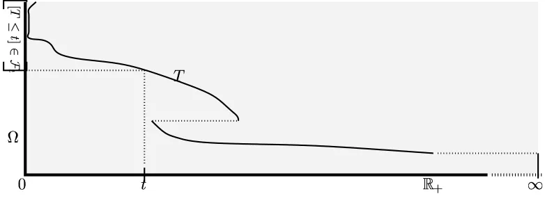
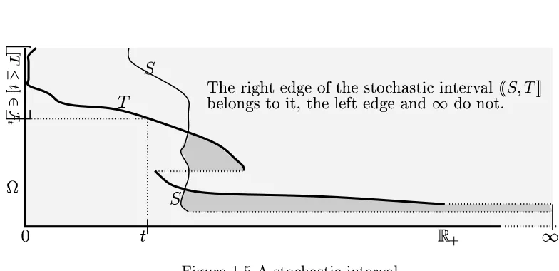
Filtrations on Measurable Spaces 21, The Base Space 22, Processes 23, Stop-ping Times and Stochastic Intervals 27, Some Examples of StopStop-ping Times 29, Probabilities 32, The Sizes of Random Variables 33, Two Notions of Equality for Processes 34, The Natural Conditions 36
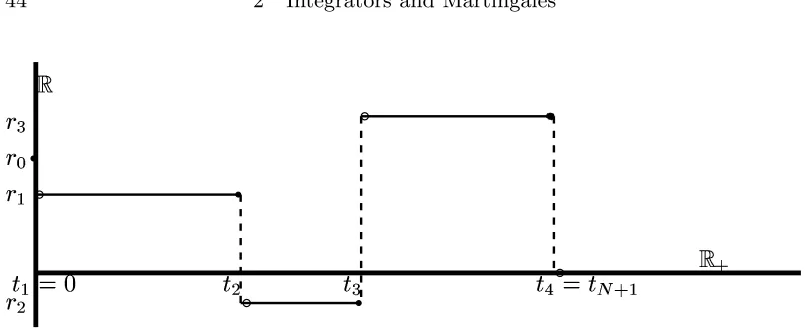
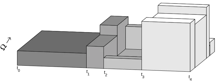
Chapter 2 Integrators and Martingales . . . 43 Step Functions and Lebesgue–Stieltjes Integrators on the Line 43
2.1 The Elementary Stochastic Integral . . . 46
Elementary Stochastic Integrands 46, The Elementary Stochastic Integral 47, The Elementary Integral and Stopping Times 47,Lp-Integrators 49, Local Properties 51
2.2 The Semivariations . . . 53
The Size of an Integrator 54, Vectors of Integrators 56, The Natural Conditions 56
2.3 Path Regularity of Integrators . . . 58
Right-Continuity and Left Limits 58, Boundedness of the Paths 61, Redefinition of Integrators 62, The Maximal Inequality 63, Law and Canonical Representation 64
2.4 Processes of Finite Variation . . . 67
Decomposition into Continuous and Jump Parts 69, The Change-of-Variable Formula 70
2.5 Martingales . . . 71
Submartingales and Supermartingales 73, Regularity of the Paths: Right-Continuity and Left Limits 74, Boundedness of the Paths 76, Doob’s Optional Stopping Theorem 77, Martingales Are Integrators 78, Martingales in Lp 80
Chapter 3 Extension of the Integral . . . 87 Daniell’s Extension Procedure on the Line 87
3.1 The Daniell Mean . . . 88
A Temporary Assumption 89, Properties of the Daniell Mean 90
3.2 The Integration Theory of a Mean . . . 94
Negligible Functions and Sets 95, Processes Finite for the Mean and Defined Almost Everywhere 97, Integrable Processes and the Stochastic Integral 99, Permanence Properties of Integrable Functions 101, Permanence Under Algebraic and Order Operations 101, Permanence Under Pointwise Limits of Sequences 102, Integrable Sets 104
viii Contents
3.3 Countable Additivity in p-Mean . . . 106
The Integration Theory of Vectors of Integrators 109
3.4 Measurability . . . 110
Permanence Under Limits of Sequences 111, Permanence Under Algebraic and Order Operations 112, The Integrability Criterion 113, Measurable Sets 114
3.5 Predictable and Previsible Processes . . . 115
Predictable Processes 115, Previsible Processes 118, Predictable Stopping Times 118, Accessible Stopping Times 122
3.6 Special Properties of Daniell’s Mean . . . 123
Maximality 123, Continuity Along Increasing Sequences 124, Predictable Envelopes 125, Regularity 128, Stability Under Change of Measure 129
3.7 The Indefinite Integral . . . 130
The Indefinite Integral 132, Integration Theory of the Indefinite Integral 135, A General Integrability Criterion 137, Approximation of the Integral via Parti-tions 138, Pathwise Computation of the Indefinite Integral 140, Integrators of Finite Variation 144
3.8 Functions of Integrators . . . 145
Square Bracket and Square Function of an Integrator 148, The Square Bracket of Two Integrators 150, The Square Bracket of an Indefinite Integral 153, Application: The Jump of an Indefinite Integral 155
3.9 Itˆo’s Formula . . . 157
The Dol´eans–Dade Exponential 159, Additional Exercises 161, Girsanov Theo-rems 162, The Stratonovich Integral 168
3.10 Random Measures . . . 171 σ-Additivity 174, Law and Canonical Representation 175, Example: Wiener Random Measure 177, Example: The Jump Measure of an Integrator 180, Strict Random Measures and Point Processes 183, Example: Poisson Point Processes 184, The Girsanov Theorem for Poisson Point Processes 185
Chapter 4 Control of Integral and Integrator . . . 187 4.1 Change of Measure — Factorization . . . 187
A Simple Case 187, The Main Factorization Theorem 191, Proof for p >0 195, Proof for p= 0 205
4.2 Martingale Inequalities . . . 209
Fefferman’s Inequality 209, The Burkholder–Davis–Gundy Inequalities 213, The Hardy Mean 216, Martingale Representation on Wiener Space 218, Additional Exercises 219
4.3 The Doob–Meyer Decomposition . . . 221
Dol´eans–Dade Measures and Processes 222, Proof of Theorem 4.3.1: Necessity, Uniqueness, and Existence 225, Proof of Theorem 4.3.1: The Inequalities 227, The Previsible Square Function 228, The Doob–Meyer Decomposition of a Random Measure 231
4.4 Semimartingales . . . 232
Integrators Are Semimartingales 233, Various Decompositions of an Integrator 234
4.5 Previsible Control of Integrators . . . 238
Controlling a Single Integrator 239, Previsible Control of Vectors of Integrators 246, Previsible Control of Random Measures 251
4.6 L´evy Processes . . . 253
Chapter 5 Stochastic Differential Equations . . . 271 5.1 Introduction . . . 271
First Assumptions on the Data and Definition of Solution 272, Example: The Ordinary Differential Equation (ODE) 273, ODE: Flows and Actions 278, ODE: Approximation 280
5.2 Existence and Uniqueness of the Solution . . . 282
The Picard Norms 283, Lipschitz Conditions 285, Existence and Uniqueness of the Solution 289, Stability 293, Differential Equations Driven by Random Measures 296, The Classical SDE 297
5.3 Stability: Differentiability in Parameters . . . 298
The Derivative of the Solution 301, Pathwise Differentiability 303, Higher Order Derivatives 305
5.4 Pathwise Computation of the Solution . . . 310
The Case of Markovian Coupling Coefficients 311, The Case of Endogenous Cou-pling Coefficients 314, The Universal Solution 316, A Non-Adaptive Scheme 317, The Stratonovich Equation 320, Higher Order Approximation: Obstructions 321, Higher Order Approximation: Results 326
5.5 Weak Solutions . . . 330
The Size of the Solution 332, Existence of Weak Solutions 333, Uniqueness 337
5.6 Stochastic Flows . . . 343
Stochastic Flows with a Continuous Driver 343, Drivers with Small Jumps 346, Markovian Stochastic Flows 347, Markovian Stochastic Flows Driven by a L´evy Process 349
5.7 Semigroups, Markov Processes, and PDE . . . 351
Stochastic Representation of Feller Semigroups 351
Appendix A Complements to Topology and Measure Theory . . . 363 A.1 Notations and Conventions . . . 363 A.2 Topological Miscellanea . . . 366
The Theorem of Stone–Weierstraß 366, Topologies, Filters, Uniformities 373, Semi-continuity 376, Separable Metric Spaces 377, Topological Vector Spaces 379, The Minimax Theorem, Lemmas of Gronwall and Kolmogoroff 382, Differentiation 388
A.3 Measure and Integration . . . 391 σ-Algebras 391, Sequential Closure 391, Measures and Integrals 394, Order-Continuous and Tight Elementary Integrals 398, Projective Systems of Mea-sures 401, Products of Elementary Integrals 402, Infinite Products of Elementary Integrals 404, Images, Law, and Distribution 405, The Vector Lattice of All Mea-sures 406, Conditional Expectation 407, Numerical and σ-Finite Measures 408, Characteristic Functions 409, Convolution 413, Liftings, Disintegration of Mea-sures 414, Gaussian and Poisson Random Variables 419
A.4 Weak Convergence of Measures . . . 421
Uniform Tightness 425, Application: Donsker’s Theorem 426
A.5 Analytic Sets and Capacity . . . 432
Applications to Stochastic Analysis 436, Supplements and Additional Exercises 440
A.6 Suslin Spaces and Tightness of Measures . . . 440
Polish and Suslin Spaces 440
A.7 The Skorohod Topology . . . 443 A.8 The Lp-Spaces . . . 448
x Contents
A.9 Semigroups of Operators . . . 463
Resolvent and Generator 463, Feller Semigroups 465, The Natural Extension of a Feller Semigroup 467 Appendix B Answers to Selected Problems . . . 470
References . . . 477
Index of Notations . . . 483
This book originated with several courses given at the University of Texas. The audience consisted of graduate students of mathematics, physics, electri-cal engineering, and finance. Most had met some stochastic analysis during work in their field; the course was meant to provide the mathematical un-derpinning. To satisfy the economists, driving processes other than Wiener process had to be treated; to give the mathematicians a chance to connect with the literature and discrete-time martingales, I chose to include driving terms with jumps. This plus a predilection for generality for simplicity’s sake led directly to the most general stochastic Lebesgue–Stieltjes integral.
The spirit of the exposition is as follows: just as having finite variation and being right-continuous identifies the useful Lebesgue–Stieltjes distribution functions among all functions on the line, are there criteria for processes to be useful as “random distribution functions.” They turn out to be straight-forward generalizations of those on the line. A process that meets these criteria is called an integrator, and its integration theory is just as easy as that of a deterministic distribution function on the line – provided Daniell’s method is used. (This proviso has to do with the lack of convexity in some of the target spaces of the stochastic integral.)
For the purpose of error estimates in approximations both to the stochastic integral and to solutions of stochastic differential equations we define various numerical sizes of an integrator Z and analyze rather carefully how they propagate through many operations done on and with Z, for instance, solving a stochastic differential equation driven by Z. These size-measurements arise as generalizations to integrators of the famed Burkholder–Davis–Gundy inequalities for martingales. The present exposition differs in the ubiquitous use of numerical estimates from the many fine books on the market, where convergence arguments are usually done in probability or every once in a while in Hilbert space L2. For reasons that unfold with the story we employ the Lp-norms in the whole range 0 ≤ p < ∞. An effort is made to furnish reasonable estimates for the universal constants that occur in this context.
Such attention to estimates, unusual as it may be for a book on this subject, pays handsomely with some new results that may be edifying even to the expert. For instance, it turns out that every integrator Z can be controlled
xii Preface
by an increasing previsible process much like a Wiener process is controlled by time t; and if not with respect to the given probability, then at least with respect to an equivalent one that lets one view the given integrator as a map into Hilbert space, where computation is comparatively facile. This previsible controller obviates prelocal arguments [91] and can be used to construct Picard norms for the solution of stochastic differential equations driven by Z that allow growth estimates, easy treatment of stability theory, and evenpathwise algorithms for the solution. These schemes extend without ado to random measures, including the previsible control and its application to stochastic differential equations driven by them.
All this would seem to lead necessarily to an enormous number of tech-nicalities. A strenuous effort is made to keep them to a minimum, by these devices: everything not directly needed in stochastic integration theory and its application to the solution of stochastic differential equations is either omitted or relegated to the Supplements or to the Appendices. A short sur-vey of the beautiful “General Theory of Processes” developed by the French school can be found there.
A warning concerning the usual conditions is appropriate at this point. They have been replaced throughout with what I call the natural conditions. This will no doubt arouse the ire of experts who think one should not “tamper with a mature field.” However, many fine books contain erroneous statements of the important Girsanov theorem – in fact, it is hard to find a correct statement in unbounded time – and this is traceable directly to the employ of the usual conditions (see example 3.9.14 on page 164 and 3.9.20). In mathematics, correctness trumps conformity. The natural conditions confer the same benefits as do the usual ones: path regularity (section 2.3), section theorems (page 437 ff.), and an ample supply of stopping times (ibidem), without setting a trap in Girsanov’s theorem.
The students were expected to know the basics of point set topology up to Tychonoff’s theorem, general integration theory, and enough functional analysis to recognize the Hahn–Banach theorem. If a fact fancier than that is needed, it is provided in appendix A, or at least a reference is given.
The exercises are sprinkled throughout the text and form an integral part. They have the following appearance:
Exercise 4.3.2 This is an exercise. It is set in a smaller font. It requires no novel argument to solve it, only arguments and results that have appeared earlier. Answers to some of the exercises can be found in appendix B. Answers to most of them can be found in appendix C, which is available on the web via http://www.ma.utexas.edu/users/cup/Answers.
http://www.ma.utexas.edu/users/cup/Errata contains the errata. I plead with the gentle reader to send me the errors he/she found via email to [email protected], so that I may include them, with proper credit of course, in these errata.
1
Introduction
1.1 Motivation: Stochastic Differential Equations
Stochastic Integration and Stochastic Differential Equations (SDEs) appear in analysis in various guises. An example from physics will perhaps best illuminate the need for this field and give an inkling of its particularities. Consider a physical system whose state at time t is described by a vector Xt
in Rn. In fact, for concreteness’ sake imagine that the system is a space probe on the way to the moon. The pertinent quantities are its location and momentum. If xt is its location at time t and pt its momentum at that
instant, then Xt is the 6-vector (xt, pt) in the phase space R6. In an ideal
world the evolution of the state is governed by a differential equation: dXt
dt =
dxt/dt
dpt/dt
=
pt/m
F(xt, pt)
.
Here m is the mass of the probe. The first line is merely the definition of p: momentum = mass × velocity. The second line is Newton’s second law: the rate of change of the momentum is the force F. For simplicity of reading we rewrite this in the form
dXt =a(Xt)dt , (1.1.1)
which expresses the idea that the change of Xt during the time-interval dt
is proportional to the time dt elapsed, with a proportionality constant or coupling coefficient a that depends on the state of the system and is provided by a model for the forces acting. In the present case a(X) is the 6-vector (p/m, F(X)). Given the initial state X0, there will be a unique solution to (1.1.1). The usual way to show the existence of this solution is Picard’s iterative scheme: first one observes that (1.1.1) can be rewritten in the form of an integral equation:
Xt =X0+ Z t
0
a(Xs)ds . (1.1.2)
Then one starts Picard’s scheme with X0
t =X0 or a better guess and defines the iterates inductively by
Xtn+1 =X0+ Z t
0
a(Xsn)ds .
If the coupling coefficient a is a Lipschitz function of its argument, then the Picard iterates Xn will converge uniformly on every bounded time-interval and the limit X∞ is a solution of (1.1.2), and thus of (1.1.1), and the only
one. The reader who has forgotten how this works can find details on pages 274–281. Even if the solution of (1.1.1) cannot be written as an analytical expression in t, there exist extremely fast numerical methods that compute it to very high accuracy. Things look rosy.
In the less-than-ideal real world our system is subject to unknown forces, noise. Our rocket will travel through gullies in the gravitational field that are due to unknown inhomogeneities in the mass distribution of the earth; it will meet gusts of wind that cannot be foreseen; it might even run into a gaggle of geese that deflect it. The evolution of the system is better modeled by an equation
dXt =a(Xt)dt+dGt , (1.1.3)
where Gt is a noise that contributes its differential dGt to the change dXt
of Xt during the interval dt. To accommodate the idea that the noise comes
from without the system one assumes that there is a background noise Zt
– consisting of gravitational gullies, gusts, and geese in our example – and that its effect on the state during the time-interval dt is proportional to the difference dZt of the cumulative noise Zt during the time-interval dt, with
a proportionality constant or coupling coefficient b that depends on the state of the system:
dGt =b(Xt)dZt .
For instance, if our probe is at time t halfway to the moon, then the effect of the gaggle of geese at that instant should be considered negligible, and the effect of the gravitational gullies is small. Equation (1.1.3) turns into
dXt =a(Xt)dt+b(Xt)dZt , (1.1.4)
in integrated form Xt =Xt0+
Z t
0
a(Xs)ds+
Z t
0
b(Xs)dZs. (1.1.5)
What is the meaning of this equation in practical terms? Since the back-ground noise Zt is not known one cannot solve (1.1.5), and nothing seems to
be gained. Let us not give up too easily, though. Physical intuition tells us that the rocket, though deflected by gullies, gusts, and geese, will probably not turn all the way around but will rather still head somewhere in the vicin-ity of the moon. In fact, for all we know the various noises might just cancel each other and permit a perfect landing.
What are the chances of this happening? They seem remote, perhaps, yet it is obviously important to find out how likely it is that our vehicle will at least hit the moon or, better, hit it reasonably closely to the intended landing site. The smaller the noise dZt, or at least its effect b(Xt)dZt, the better
1.1 Motivation: Stochastic Differential Equations 3 a statistical inference: from some reasonable or measurable assumptions on the background noise Z or its effect b(X)dZ we hope to conclude about the likelihood of a successful landing.
This is all a bit vague. We must cast the preceding contemplations in a mathematical framework in order to talk about them with precision and, if possible, to obtain quantitative answers. To this end let us introduce the set Ω of all possible evolutions of the world. The idea is this: at the beginning t= 0 of the reckoning of time we may or may not know the state-of-the-world ω0, but thereafter the course that the history ω :t7→ωt of the
world actually will take has the vast collection Ω of evolutions to choose from. For any two possible courses-of-history1ω :t7→ωt and ω0:t 7→ωt0 the
state-of-the-world might take there will generally correspond different cumulative background noises t 7→Zt(ω) and t 7→Zt(ω0). We stipulate further that
there is a function P that assigns to certain subsets E of Ω , the events, a probability P[E] that they will occur, i.e., that the actual evolution lies in E. It is known that no reasonable probability P can be defined on all subsets of Ω . We assume therefore that the collection of all events that can ever be observed or are ever pertinent form a σ-algebra F of subsets of Ω and that the function P is a probability measure on F. It is not altogether easy to defend these assumptions. Why should the observable events form a σ-algebra? Why should P be σ-additive? We content ourselves with this answer: there is a well-developed theory of such triples (Ω,F,P); it comprises a rich calculus, and we want to make use of it. Kolmogorov [57] has a better answer:
Project 1.1.1 Make a mathematical model for the analysis of random phenomena that does not require σ-additivity at the outset but furnishes it instead.
So, for every possible course-of-history1 ω ∈ Ω there is a background noise Z. :t 7→Zt(ω), and with it comes the effective noise b(Xt)dZt(ω) that our
system is subject to during dt. Evidently the state Xt of the system depends
on ω as well. The obvious thing to do here is to compute, for every ω ∈Ω , the solution of equation (1.1.5), to wit,
Xt(ω) =Xt0+
Z t
0
a(Xs(ω))ds+
Z t
0
b(Xs(ω))dZs(ω), (1.1.6)
as the limit of the Picard iterates X0
t def=X0, Xtn+1(ω)def
=Xt0+ Z t
0
a(Xsn(ω))ds+ Z t
0
b(Xsn(ω))dZs(ω). (1.1.7)
Let T be the time when the probe hits the moon. This depends on chance, of course: T =T(ω) . Recall that xt are the three spatial components of Xt. 1 The redundancy in these words is for emphasis. [Note how repeated references to a
Our interest is in the function ω 7→xT(ω) =xT(ω)(ω), the location of the probe at the time T. Suppose we consider a landing successful if our probe lands within F feet of the ideal landing site s at the time T it does land. We are then most interested in the probability
pF def
= P {ω ∈Ω :xT(ω)−s< F}
of a successful landing – its value should influence strongly our decision to launch. Now xT is just a function on Ω , albeit defined in a circuitous way. We should be able to compute the set {ω ∈Ω :kxT(ω)−sk< F}, and if we have enough information about P, we should be able to compute its probability pF and to make a decision. This is all classical ordinary differential equations (ODE), complicated by the presence of a parameter ω: straightforward in principle, if possibly hard in execution.
The Obstacle
As long as the paths Z.(ω) : s 7→ Zs(ω) of the background noise are
right-continuous and have finite variation, the integrals R · · ·sdZs
appear-ing in equations (1.1.6) and (1.1.7) have a perfectly clear classical meanappear-ing as Lebesgue–Stieltjes integrals, and Picard’s scheme works as usual, under the assumption that the coupling coefficients a, b are Lipschitz functions (see pages 274–281).
Now, since we do not know the background noise Z precisely, we must make a model about its statistical behavior. And here a formidable ob-stacle rears its head: the simplest and most plausible statistical assumptions about Z force it to be so irregular that the integrals of (1.1.6) and (1.1.7) can-not be interpreted in terms of the usual integration theory. The moment we stipulate some symmetry that merely expresses the idea that we don’t know it all, obstacles arise that cause the paths of Z to have infinite variation and thus prevent the use of the Lebesgue–Stieltjes integral in giving a meaning to expressions like R Xs dZs(ω) .
Here are two assumptions on the randomdriving term Z that are eminently plausible:
(a) The expectation of the increment dZt ≈ Zt+h −Zt should be zero;
otherwise there is a drift part to the noise, which should be subsumed in the first driving term R ·ds of equation (1.1.6). We may want to assume a bit more, namely, that if everything of interest, including the noise Z.(ω) , was actually observed up to time t, then the future increment Zt+h −Zt still
averages to zero. Again, if this is not so, then a part of Z can be shifted into a driving term of finite variation so that the remainder satisfies this condition – see theorem 4.3.1 on page 221 and proposition 4.4.1 on page 233. The mathematical formulation of this idea is as follows: let Ft be the σ-algebra
1.1 Motivation: Stochastic Differential Equations 5 time t; Ft is commonly and with intuitive appeal called the history or past
at time t. In these terms our assumption is that the conditional expectation
EZt+h−Zt
Ft
of the future differential noise given the past vanishes. This makes Z a martingale on the filtration F.={Ft}0≤t<∞ – these notions are discussed in
detail in sections 1.3 and 2.5.
(b) We may want to assume further that Z does not change too wildly with time, say, that the paths s 7→ Zs(ω) are continuous. In the example
of our space probe this reflects the idea that it will not blow up or be hit by lightning; these would be huge and sudden disturbances that we avoid by careful engineering and by not launching during a thunderstorm.
A background noise Z satisfying (a) and (b) has the property thatalmost none of its paths Z.(ω) is differentiable at any instant – see exercise 3.8.13 on page 152. By a well-known theorem of real analysis,2 the path s 7→Zs(ω)
does not have finite variation on any time-interval; and this irregularity happens for almost every ω∈Ω !
We are stumped: since s7→Zs does not have finite variation, the integrals
R
· · ·dZs appearing in equations (1.1.6) and (1.1.7) do not make sense in any
way we know, and then neither do the equations themselves.
Historically, the situation stalled at this juncture for quite a while. Wiener made an attempt to define the integrals in question in the sense of distribution theory, but the resultingWiener integral is unsuitable for the iteration scheme (1.1.7), for lack of decent limit theorems.
Itˆ
o’s Way Out of the Quandary
The problem is evidently to give a meaning to the integrals appearing in (1.1.6) and (1.1.7). Not only that, any prospective integral must have rather good properties: to show that the iterates Xn of (1.1.7) form a Cauchy sequence and thus converge there must be estimates available; to show that their limit is the solution of (1.1.6) there must be a limit theorem that permits the interchange of limit and integral, to wit,
Z t
0 lim
n b X n s
dZs = lim
n
Z t
0
b XsndZs .
In other words, what is needed is an integral satisfying the Dominated Con-vergence Theorem, say. Convinced that an integral with this property cannot be defined pathwise, i.e., ω for ω, the Japanese mathematician Itˆo decided to try for an integral in the sense of the L2-mean. His idea was this: while the sums
SP(ω)def =
K
X
k=1
b Xσk(ω)
Zsk+1(ω)−Zsk(ω)
, sk ≤σk ≤sk+1, (1.1.8)
which appear in the usual definition of the integral, do not converge for any ω ∈ Ω , there may obtain convergence in mean as the partition P ={s0 < s1 < . . . < sK+1} is refined. In other words, there may be a ran-dom variable I such that
kSP −IkL2 →0 as mesh[P]→0.
And if SP should not converge in L2-mean, it may converge in Lp-mean for some other p∈(0,∞), or at least in measure (p = 0 ).
In fact, this approach succeeds, but not without another observation that Itˆo made: for the purpose of Picard’s scheme it is not necessary to integrate all processes.3 An integral defined for non-anticipating integrands suffices. In order to describe this notion with a modicum of precision, we must refer again to the σ-algebras Ft comprising the history known at time t. The integrals
Rt
0 a(X0)ds=a(X0)·t and Rt
0b(X0)dZs(ω) =b(X0)· Zt(ω)−Z0(ω)
are at any time measurable on Ft because Zt is; then so is the first Picard iterate
X1
t . Suppose it is true that the iterate Xn of Picard’s scheme is at all
times t measurable on Ft; then so are a(Xtn) and b(Xtn) . Their integrals,
being limits of sums as in (1.1.8), will again be measurable on Ft at all
instants t; then so will be the next Picard iterate Xtn+1 and with it a(Xtn+1) and b(Xtn+1) , and so on. In other words, the integrands that have to be dealt withdo not anticipate the future; rather, they are at any instant t measurable on the past Ft. If this is to hold for the approximation of (1.1.8) as well,
we are forced to choose for the point σi at which b(X) is evaluated the left
endpoint si−1. We shall see in theorem 2.5.24 that the choice σi = si−1 permits martingale4 drivers Z – recall that it is the martingales that are causing the problems.
Since our object is to obtain statistical information, evaluating integrals and solving stochastic differential equations in the sense of a mean would pose no philosophical obstacle. It is, however, now not quite clear what it is that equation (1.1.5) models, if the integral is understood in the sense of the mean. Namely, what is the mechanism by which the random variable dZt affects the
change dXt in mean but not through its actual realization dZt(ω) ? Do the
possible but not actually realized courses-of-history1 somehow influence the behavior of our system? We shall return to this question in remarks 3.7.27 on page 141 and give a rather satisfactory answer in section 5.4 on page 310.
Summary: The Task Ahead
It is now clear what has to be done. First, the stochastic integral in the Lp-mean sense for non-anticipating integrands has to be developed. This 3A process is simply a functionY : (s, ω)7→Y
1.1 Motivation: Stochastic Differential Equations 7 is surprisingly easy. As in the case of integrals on the line, the integral is defined first in a non-controversial way on a collection E of elementary integrands. These are the analogs of the familiar step functions. Then that elementary integral is extended to a large class of processes in such a way that it features the Dominated Convergence Theorem. This is not possible for arbitrary driving terms Z, just as not every function z on the line is the distribution function of a σ-additive measure – to earn that distinction z must be right-continuous and have finite variation. The stochastic driving terms Z for which an extension with the desired properties has a chance to exist are identified by conditions completely analogous to these two and are called integrators.
For the extension proper we employ Daniell’s method. The arguments are so similar to the usual ones that it would suffice to state the theorems, were it not for the deplorable fact that Daniell’s procedure is generally not too well known, is even being resisted. Its efficacy is unsurpassed, in particular in the stochastic case.
Then it has to be shown that the integral found can, in fact, be used to solve the stochastic differential equation (1.1.5). Again, the arguments are straightforward adaptations of the classical ones outlined in the beginning of section 5.1, jazzed up a bit in the manner well known from the theory of ordinary differential equations in Banach spaces e.g., [22, page 279 ff.] – the reader need not be familiar with it, as the details are developed in chapter 5. A pleasant surprise waits in the wings. Although the integrals appearing in (1.1.6) cannot be understood pathwise in the ordinary sense, there is an algorithm that solves (1.1.6) pathwise, i.e., ω–by–ω. This answers satisfactorily the question raised above concerning the meaning of solving a stochastic differential equation “in mean.”
Indeed, why not let the cat out of the bag: the algorithm is simply the method of Euler–Peano. Recall how this works in the case of the deterministic differential equation dXt = a(Xt)dt. One gives oneself a threshold δ and
defines inductively an approximate solution Xt(δ) at the points tk def= kδ,
k ∈ N, as follows: if Xt(kδ) is constructed, wait until the driving term t has changed by δ, and let tk+1 def= tk+δ and
Xt(kδ+1) =Xt(kδ)+a(Xt(kδ))×(tk+1−tk) ;
between tk and tk+1 define Xt(δ) by linearity. The compactness criterion
A.2.38 of Ascoli–Arzel`a allows the conclusion that the polygonal paths X(δ) have a limit point as δ → 0 , which is a solution. This scheme actually expresses more intuitively the meaning of the equation dXt =a(Xt)dt than
and Xt(kδ+1) , does converge for almost all ω ∈ Ω in the stochastic case, when the deterministic driving term t 7→ t is replaced by the stochastic driver t 7→Zt(ω) (see section 5.4).
So now the reader might well ask why we should go through all the labor of stochastic integration: integrals do not even appear in this scheme! And the question of what it means to solve a stochastic differential equation “in mean” does not arise. The answer is that there seems to be no way to prove the almost sure convergence of the Euler–Peano scheme directly, due to the absence of compactness. One has to show5 that the Picard scheme works before the Euler–Peano scheme can be proved to converge.
So here is a new perspective: what we mean by a solution of equa-tion (1.1.4),
dXt(ω) =a(Xt(ω))dt+b(Xt(ω))dZt(ω),
is a limit to the Euler–Peano scheme. Much of the labor in these notes is expended just to establish via stochastic integration and Picard’s method that this scheme does, in fact, converge almost surely.
Two further points. First, even if the model for the background noise Z is simple, say, is a Wiener process, the stochastic integration theory must be developed for integrators more general than that. The reason is that the solution of a stochastic differential equation is itself an integrator, and in this capacity it can best be analyzed. Moreover, in mathematical finance and in filtering and control theory, the solution of one stochastic differential equation is often used to drive another.
Next, in most applications the state of the system will have many compo-nents and there will be several background noises; the stochastic differential equation (1.1.5) then becomes6
Xtν =Ctν + X 1≤η≤d
Z t
0
Fην[X1, . . . , Xn]dZη , ν = 1, . . . , n .
The state of the system is a vector X = (Xν)ν=1...n in Rn whose evolution
is driven by a collection Zη : 1≤η≤d of scalar integrators. The d vector fields Fη = (Fην)ν=1...n are the coupling coefficients, which describe the effect
of the background noises Zη on the change of X. Ct = (Ctν)ν=1...n is the
initial condition – it is convenient to abandon the idea that it be constant. It eases the reading to rewrite the previous equation in vector notation as7
Xt =Ct+
Z t
0
Fη[X]dZη . (1.1.9)
5So far – here is a challenge for the reader!
6See equation (5.2.1) on page 282 for a more precise discussion.
7We shall use theEinstein convention throughout: summation over repeated indicesin
1.2 Wiener Process 9 The form (1.1.9) offers an intuitive way of reading the stochastic differential equation: the noise Zη drives the state X in the direction Fη[X] . In our
example we had four driving terms: Z1
t = t is time and F1 is the systemic force; Z2 describes the gravitational gullies and F2 their effect; and Z3 and Z4 describe the gusts of wind and the gaggle of geese, respectively. The need for several noises will occasionally call for estimates involving whole slews {Z1, ..., Zd} of integrators.
1.2 Wiener Process
Wiener process8 is the model most frequently used for a background noise. It can perhaps best be motivated by looking at Brownian motion, for which it was an early model. Brownian motion is an example not far removed from our space probe, in that it concerns the motion of a particle moving under the influence of noise. It is simple enough to allow a good stab at the background noise.
Example 1.2.1 (Brownian Motion) Soon after the invention of the microscope in the 17th century it was observed that pollen immersed in a fluid of its own specific weight does not stay calmly suspended but rather moves about in a highly irregular fashion, and never stops. The English physicist Brown studied this phenomenon extensively in the early part of the 19th century and found some systematic behavior: the motion is the more pronounced the smaller the pollen and the higher the temperature; the pollen does not aim for any goal – rather, during any time-interval its path appears much the same as it does during any other interval of like duration, and it also looks the same if the direction of time is reversed. There was speculation that the pollen, being live matter, is propelling itself through the fluid. This, however, runs into the objection that it must have infinite energy to do so (jars of fluid with pollen in it were stored for up to 20 years in dark, cool places, after which the pollen was observed to jitter about with undiminished enthusiasm); worse, ground-up granite instead of pollen showed the same behavior.
In 1905 Einstein wrote three Nobel-prize–worthy papers. One offered the Special Theory of Relativity, another explained the Photoeffect (for this he got the Nobel prize), and the third gave an explanation of Brownian motion. It rests on the idea that the pollen is kicked by the much smaller fluid molecules, which are in constant thermal motion. The idea is not, as one might think at first, that the little jittery movements one observes are due to kicks received from particularly energetic molecules; estimates of the distribution of the kinetic energy of the fluid molecules rule this out. Rather, it is this: the pollen suffers an enormous number of collisions with the molecules of the surrounding fluid, each trying to propel it in a different direction, but mostly canceling each other; the motion observed is due to
statistical fluctuations. Formulating this in mathematical terms leads to a stochastic differential equation9
dxt
dpt
=
pt/m dt
−α pt dt + dWt
(1.2.1) for the location (x, p) of the pollen in its phase space. The first line expresses merely the definition of the momentum p; namely, the rate of change of the location x in R3 is the velocity v = p/m, m being the mass of the pollen. The second line attributes the change of p during dt to two causes: −αp dt describes the resistance to motion due to the viscosity of the fluid, and dWt is
the sum of the very small momenta that the enormous number of collisions impart to the pollen during dt. The random driving term is denoted W
here rather than Z as in section 1.1, since the model for it will be a Wiener process.
This explanation leads to a plausible model for the background noise W: dWt = Wt+dt − Wt is the sum of a huge number of exceedingly small
momenta, so by the Central Limit Theorem A.4.4 we expect dWt to have
a normal law. (For the notion of a law or distribution see section A.3 on page 391. We won’t discuss here Lindeberg’s or other conditions that would make this argument more rigorous; let us just assume that whatever condition on the distribution of the momenta of the molecules needed for the CLT is satisfied. We are, after all, doing heuristics here.)
We do not see any reason why kicks in one direction should, on the average, be more likely than in any other, so this normal law should have expectation zero and a multiple of the identity for its covariance matrix. In other words, it is plausible to stipulate that dW be a 3-vector of identically distributed independent normal random variables. It suffices to analyze one of its three scalar components; let us denote it by dW.
Next, there is no reason to believe that the total momenta imparted during non-overlapping time-intervals should have anything to do with one another. In terms of W this means that for consecutive instants 0 = t0 < t1 < t2 < . . . < tK the corresponding family of consecutive increments
n
Wt1 −Wt0, Wt2−Wt1, . . . , WtK −WtK−1 o
should be independent. In self-explanatory terminology: we stipulate that
W have independent increments.
The background noise that we visualize does not change its character with time (except when the temperature changes). Therefore the law of Wt−Ws
should not depend on the times s, t individually but only on their difference, the elapsed time t−s. In self-explanatory terminology: we stipulate that W
be stationary.
9 Edward Nelson’s book, Dynamical Theories of Brownian Motion [82], offers a most
1.2 Wiener Process 11 SubtractingW0 does not change the differential noises dWt, so we simplify
the situation further by stipulating that W0 = 0 .
Let δ =var(W1) =E[W12] . The variances of W(k+1)/n−Wk/n then must
be δ/n, since they are all equal by stationarity and add up to δ by the independence of the increments. Thus the variance of Wq is δq for a rational
q =k/n. By continuity the variance of Wt is δt, and the stationarity forces
the variance of Wt −Ws to be δ(t−s) .
Our heuristics about the cause of the Brownian jitter have led us to a stoch-astic differential equation, (1.2.1), including a model for the driving term W with rather specific properties: it should have stationary independent incre-ments dWt distributed as N(0, δ·dt) and have W0 = 0 .
Does such a background noise exist? Yes; see theorem 1.2.2 below. If so, what further properties does it have? Volumes; see, e.g., [47]. How many such noises are there? Essentially one for every diffusion coefficient δ (see lemma 1.2.7 on page 16 and exercise 1.2.14 on page 19). They are called Wiener processes.
Existence of Wiener Process
What is meant by “Wiener process8 exists”? It means that there is a probability space (Ω,F,P) on which there lives a family {Wt : t ≥ 0}
of random variables with the properties specified above. The quadruple Ω,F,P,{Wt :t≥0}
is a mathematical model for the noise envisaged.
The case δ= 1 is representative (exercise 1.2.14), so we concentrate on it: Theorem 1.2.2 (Existence and Continuity of Wiener Process) (i) There exist a probability space (Ω,F,P) and on it a family {Wt : 0≤t <∞} of random
variables that has stationary independent increments, and such that W0 = 0 and the law of the increment Wt −Ws is N(0, t−s).
(ii) Given such a family, one may change every Wt on a negligible set
in such a way that for every ω ∈ Ω the path t 7→ Wt(ω) is a continuous
function.
Definition 1.2.3 Any family Wt : t ∈ [0,∞) of random variables (defined
on some probability space) that has continuous paths and stationary indepen-dent increments Wt −Ws with law N(0, t−s), and that is normalized to
W0 = 0, is called a standard Wiener process.
A standard Wiener process can be characterized more simply as a continuous martingale W scaled by W0 = 0 and E[Wt2] = t (see corollary 3.9.5).
the distribution of the prime numbers – alas, so far it is reluctant to part with this knowledge. Wiener process is frequently called Brownian motion in the literature. We prefer to reserve the name “Brownian motion” for the physical phenomenon described in example 1.2.1 and capable of being described to various degrees of accuracy by different mathematical models [82].
Proof of Theorem 1.2.2 (i). To get an idea how we might construct the probability space (Ω,F,P) and the Wt, consider dW as a map that associates
with any interval (s, t] the random variable Wt−Ws on Ω , i.e., as a measure
on [0,∞) with values in L2(P) . It is after all in this capacity that the noise W will be used in a stochastic differential equation (see page 5). Eventually we shall need to integrate functions with dW, so we are tempted to extend this measure by linearity to a map R ·dW from step functions
φ=X
k
rk·1(tk,tk+1] on the half-line to random variables in L2(P) via
Z
φ dW =X
k
rk·(Wtk+1 −Wtk).
Suppose that the family {Wt : 0 ≤ t < ∞} has the properties listed
in (i). It is then rather easy to check that R · dW extends to a linear isometry U from L2[0,∞) to L2(P) with the property that U(φ) has a normal law N(0, σ2) with mean zero and variance σ2 =R0∞φ2(x)dx, and so that functions perpendicular in L2[0,∞) have independent images in L2(P) . If we apply U to a basis of L2[0,∞) , we shall get a sequence (ξ
n) of
independent N(0,1) random variables. The verification of these claims is left as an exercise.
We now stand these heuristics on their head and arrive at the
Construction of Wiener ProcessLet (Ω,F,P) be a probability space that ad-mits a sequence (ξn) of independent identically distributed random variables,
each having law N(0,1) . This can be had by the following simple construc-tion: prepare countably many copies of (R,B•(R), γ
1)10 and let (Ω,F,P) be their product; for ξn take the nth coordinate function. Now pick any
orthonormal basis (φn) of the Hilbert space L2[0,∞) . Any element f of
L2[0,∞) can be written uniquely in the form f =P∞n=1anφn ,
with kfk2
L2[0,∞) = P∞
n=1a2n <∞. So we may define a map Φ by
Φ(f) =P∞n=1anξn . 10 B•(R) is theσ-algebra of Borel sets on the line, andγ
1(dx) = (1/√2π)·e−x
2/2
1.2 Wiener Process 13 Φ evidently associates with every class in L2[0,∞) an equivalence class of square integrable functions in L2(P) =L2(Ω,F,P) . Recall the argument: the finite sums PNn=1anξn form a Cauchy sequence in the space L2(P) , because
EhPNn=Manξn
2i
=PNn=Ma2n≤P∞n=Ma2n −−−−→M→∞ 0.
Since the space L2(P) is complete there is a limit in 2-mean; since L2(P) , the space of equivalence classes, is Hausdorff, this limit is unique. Φ is clearly a linear isometry from L2[0,∞) into L2(P) . It is worth noting here that our recipe Φ does not produce a function but merely an equivalence class modulo P-negligible functions. It is necessary to make some hard estimates to pick a suitable representative from each class, so as to obtain actual random variables (see lemma A.2.37).
Let us establish next that the law of Φ(f) is N(0,kfk2
L2[0,∞)) . To this end note that f =Pnanφn has the same norm as Φ(f) :
Z ∞
0
f2(t)dt=Xa2n =E[(Φ(f))2]. The simple computation
EheiαΦ(f)i =Eheiα P
nanξni =Y
n
Eheiαanξni =e−α 2P
na 2 n/2
shows that the characteristic function of Φ(f) is that of a N(0,Pa2n) random variable (see exercise A.3.45 on page 419). Since the characteristic function determines the law (page 410), the claim follows.
A similar argument shows that if f1, f2, . . . are orthogonal in L2[0,∞) , then Φ(f1),Φ(f2), . . . are not only also orthogonal in L2(P) but are actually independent:
clearly Pkαkfk
2
L2[0,∞) = P
kα2k· kfkk2L2[0,∞), whence Ehei
P
kαkΦ(fk)i =EheiΦ( P
kαkfk)i =e−k P
kαkfkk 2
2
=Y
ke
−α2k·kfkk2/2
=Y
kE
h
eiαkΦ(fk)i.
This says that the joint characteristic function is the product of the marginal characteristic functions, so the random variables are independent (see exer-cise A.3.36).
For any t ≥0 let ˙Wt be the class Φ 1[0,t]
and simply pick a member Wt
of ˙Wt. If 0 ≤ s < t, then ˙Wt −W˙s = Φ 1(s,t]
is distributed N(0, t−s) and our family {Wt} is stationary. With disjoint intervals being orthogonal
Proof of Theorem 1.2.2 (ii). We start with the following observation: due to exercise A.3.47, the curve t7→ W˙t is continuous from R+ to the space Lp(P) , for any p <∞. In particular, for p= 4
E|Wt−Ws|4= 4· |t−s|2 . (1.2.2)
Next, in order to have the parameter domain open let us extend the process ˙
Wt constructed in part (i) of the proof to negative times by ˙W−t = ˙Wt for
t > 0 . Equality (1.2.2) is valid for any family {Wt : t ≥ 0} as in
theo-rem 1.2.2 (i). Lemma A.2.37 applies, with (E, ρ) = (R,| |) , p = 4 , β = 1 , C = 4 : there is a selection Wt ∈ W˙t such that the path t → Wt(ω) is
continuous for all ω ∈ Ω . We modify this by setting W.(ω) ≡ 0 in the negligible set of those points ω where W0(ω) 6= 0 and then forget about negative times.
Uniqueness of Wiener Measure
A standard Wiener process is, of course, not unique: given the one we constructed above, we paint every element of Ω purple and get a new Wiener process that differs from the old one simply because its domain Ω is different. Less facetious examples are given in exercises 1.2.14 and 1.2.16. What is unique about a Wiener process is its law or distribution.
Recall – or consult section A.3 for – the notion of the law of a real-valued random variable f : Ω → R. It is the measure f[P] on the codomain of f,
R in this case, that is given by f[P](B)def
= P[f−1(B)] on Borels B ∈ B•(R).
Now any standard Wiener process W. on some probability space (Ω,F,P) can be identified in a natural way with a random variable W that has values in the space C =C[0,∞) of continuous real-valued functions on the half-line. Namely, W is the map that associates with every ω ∈Ω the function orpath w = W(ω) whose value at t is wt = Wt(w)def= Wt(ω) , t ≥ 0 . We also call
W a representationof W. on path space.11 It is determined by the equation Wt◦W(ω) =Wt(ω), t≥0, ω ∈Ω.
Wiener measure is the law or distribution of this C-valued random vari-able W, and this will turn out to be unique.
Before we can talk about this law, we have to identify the equivalent of the Borel sets B ⊂ R above. To do this a little analysis of path space
C = C[0,∞) is required. C has a natural topology, to wit, the topology of uniform convergence on compact sets. It can be described by a metric, for instance,12
d(w, w0) = X
n∈N
sup 0≤s≤n
ws−w0s∧2−n for w, w0 ∈C . (1.2.3)
1.2 Wiener Process 15 Exercise 1.2.4 (i) A sequence (w(n)) in C converges uniformly on compact sets
to w∈C if and only if d(w(n), w)→0. C is complete under the metric d.
(ii) C is Hausdorff, and is separable, i.e., it contains a countable dense subset.
(iii) Let {w(1), w(2), . . .} be a countable dense subset of C. Every open subset
of C is the union of balls in the countable collection
Bq(w(n))def=
w:d(w, w(n))< q ff
, n∈N, 0< q∈Q.
Being separable and complete under a metric that defines the topology makes
C a polish space. The Borel σ-algebra B•(C) on C is, of course, the
σ-algebra generated by this topology (see section A.3 on page 391). As to our standard Wiener process W, defined on the probability space (Ω,F,P) and identified with a C-valued map W on Ω , it is not altogether obvious that inverse images W−1(B) of Borel sets B ⊂ C belong to F; yet this is precisely what is needed if the law W[P] of W is to be defined, in analogy with the real-valued case, by
W[P](B)def
= P[W−1(B)], B ∈ B•(C).
Let us show that they do. To this end denote by F0
∞[C] the σ-algebra
on C generated by the real-valued functions Wt : w 7→ wt, t ∈ [0,∞) , the
evaluation maps. Since Wt◦W =Wt is measurable on Ft, clearly
W−1(E)∈ F, ∀E ∈ F∞0 [C]. (1.2.4) Let us show next that every ball Br(w(0))def=
n
w : d(w, w(0))< ro belongs to F0
∞[C] . To prove this it evidently suffices to show that for fixed w(0) ∈C
the map w 7→ d(w, w(0)) is measurable on F0
∞[C] . A glance at
equa-tion (1.2.3) reveals that this will be true if for every n ∈ N the map w 7→ sup0≤s≤n|ws−ws(0)| is measurable on F∞0 [C] . This, however, is clear, since
the previous supremum equals the countable supremum of the functions w7→wq−wq(0)
, q∈Q, q ≤n , each of which is measurable on F0
∞[C] . We conclude with exercise 1.2.4 (iii)
that every open set belongs to F0
∞[C] , and that therefore
F0
∞[C] =B• C
. (1.2.5)
In view of equation (1.2.4) we now know that the inverse image under W : Ω→C of a Borel set in C belongs to F. We are now in position to talk about the image W[P] :
W[P](B)def
= P[W−1(B)], B ∈ B•(C).
Definition 1.2.5 The law of a standard Wiener process Ω,F,P, W., that is to say the probability W=W[P] on C given by
W(B)def
= W[P](B) =P[W−1(B)], B∈ B•(C),
is called Wiener measure. The topological space C equipped with Wiener measure W on its Borel sets is calledWiener space. The real-valued random variables on C that map a path w∈C to its value at t and that are denoted by Wt above, and often simply by wt, constitute the canonical Wiener
process.8
Exercise 1.2.6 The name is justified by the observation that the quadruple (C,B•(C),W,{W
t}0≤t<∞) is a standard Wiener process.
Definition 1.2.5 makes sense only if any two standard Wiener processes have the same distribution on C. Indeed they do:
Lemma 1.2.7 Any two standard Wiener processes have the same law.
Proof. Let (Ω,F,P, W.) and (Ω0,F0,P0, W.0) be two standard Wiener
pro-cesses and let W denote the law of W.. Consider a complex-valued function on C =C[0,∞) of the form
φ(w) = expi
K
X
k=1
rk(wtk−wtk−1)
= expi
K
X
k=1
rk(Wtk(w)−Wtk−1(w))
, (1.2.6) rk ∈R, 0 =t0 < t1 < . . . < tK. Its W-integral can be computed:
Z
φ(w)W(dw) = Z
expi
K
X
k=1
rk(Wtk ◦W −Wtk−1 ◦W)
dP
by independence: =
K
Y
k=1 Z
exp irk(Wtk−Wtk−1)
dP
=
K
Y
k
Z ∞
−∞
eirkx· e
−x2/2(tk−tk−1) p
2π(tk−tk−1) dx
by exercise A.3.45: = K
Y
k
e−r2k(tk−tk−1)/2 .
The same calculation can be done for P0 and shows that its distribution W0
under W0 coincides with W on functions of the form (1.2.6). Now note that these functions are bounded, and that their collection M is closed under multiplication and complex conjugation and generates the same σ-algebra as the collection {Wt : t≥0}, to wit F∞0 [C] =B• C[0,∞)
1.2 Wiener Process 17 Namely, the vector space V of bounded complex-valued functions on C on which W and W0 agree is sequentially closed and contains M, so it contains every bounded B• C[0,∞)-measurable function.
Non-Differentiability of the Wiener Path
The main point of the introduction was that a novel integration theory is needed because the driving term of stochastic differential equations occurring most frequently, Wiener process, has paths of infinite variation. We show this now. In fact,2 since a function that has finite variation on some interval is differentiable at almost every point of it, the claim is immediate from the following result:
Theorem 1.2.8 (Wiener) Let W be a standard Wiener process on some probability space (Ω,F,P). Except for the points ω in a negligible subset N
of Ω, the path t7→Wt(ω) is nowhere differentiable.
Proof [27]. Suppose that t 7→ Wt(ω) is differentiable at some instant s.
There exists a K ∈N with s < K−1 . There exist M, N ∈N such that for all n ≥ N and all t ∈ (s−5/n, s+ 5/n) , |Wt(ω)−Ws(ω)| ≤ M · |t−s|.
Consider the first three consecutive points of the form j/n, j ∈ N, in the interval (s, s+ 5/n) . The triangle inequality produces
|Wj+1
n (ω)−W j
n(ω)| ≤ |W j+1
n (ω)−Ws(ω)|+|W j
n(ω)−Ws(ω)| ≤7M/n for each of them. The point ω therefore lies in the set
N =[
K [ M [ N \
n≥N
[
k≤K·n k\+2
j=k
h |Wj+1
n −W j
n| ≤7M/n i
.
To prove that N is negligible it suffices to show that the quantity Qdef
=Ph \
n≥N
[
k≤K·n k\+2
j=k
h |Wj+1
n −W j
n| ≤7M/n ii
≤lim inf
n→∞ P
h [
k≤K·n k\+2
j=k
h |Wj+1
n −W j
n| ≤7M/n ii
vanishes. To see this note that the eventsh |Wj+1
n −W j
n| ≤7M/n i
, j =k, k+ 1, k+ 2, are independent and have probability
Ph|W1
n| ≤7M/n i
= p 1 2π/n
Z +7M/n
−7M/n
e−x2n/2dx
= √1 2π
Z +7M/√n
−7M/√n
e−ξ2/2dξ ≤ √14M 2πn .
Thus Q≤lim inf
n→∞ K·n·
const
√ n
Remark 1.2.9 In the beginning of this section Wiener process8 was motivated as a driving term for a stochastic differential equation describing physical Brownian motion. One could argue that the non-differentiability of the paths was a result of overly much idealization. Namely, the total momentum imparted to the pollen (in our billiard ball model) during the time-interval [0, t] by collisions with the gas molecules is in reality a function of finite variation in t. In fact, it is constant between kicks and jumps at a kick by the momentum imparted; it is, in particular, not continuous. If the interval dt is small enough, there will not be any kicks at all. So the assumption that the differential of the driving term is distributed N(0, dt) is just too idealistic. It seems that one should therefore look for a better model for the driver, one that takes the microscopic aspects of the interaction between pollen and gas molecules into account.
Alas, no one has succeeded so far, and there is little hope: first, the total variation of a momentum transfer during [0, t] turns out to be huge, since it does not take into account the cancellation of kicks in opposite directions. This rules out any reasonable estimates for the convergence of any scheme for the solution of the stochastic differential equation driven by a more accurately modeled noise, in terms of this variation. Also, it would be rather cumbersome to keep track of the statistics of such a process of finite variation if its structure between any two of the huge number of kicks is taken into account.
We shall therefore stick to Wiener process as a model for the driver in the model for Brownian motion and show that the statistics of the solution of equation (1.2.1) on page 10 are close to the statistics of the solution of the corresponding equation driven by a finite variation model for the driver, provided the number of kicks is sufficiently large (exercise A.4.14). We shall return to this circle of problems several times, next in example 2.5.26 on page 79.
Supplements and Additional Exercises
Fix a standard Wiener process W. on some probability space (Ω,F,P) . For any s let F0
s[W.] denote the σ-algebra generated by the collection
{Wr : 0 ≤ r ≤ s}. That is to say, Fs0[W.] is the smallest σ-algebra on
which the Wr : r ≤ s are all measurable. Intuitively, Ft0[W.] contains all
information about the random variables Ws that can be observed up to and
including time t. The collection
F.0[W.] ={Fs0[W.] : 0≤s < ∞}
of σ-algebras is called the basic filtration of the Wiener process W.. Exercise 1.2.10 F0
s[W.] increases with s and is the σ-algebra generated by
the increments {Wr−Wr0 : 0≤r, r0 ≤s}. For s < t, Wt −Ws is independent
of Fs0[W.]. Also, for 0≤s < t <∞, E[Wt|Fs0[W.]] =Ws and E
ˆ
Wt2−Ws2|Fs0[W.]
˜
1.2 Wiener Process 19
Equations (1.2.7) say that both Wt and Wt2 −t are martingales4 on F.0[W.].
Together with the continuity of the path they determine the law of the whole process W uniquely. This fact, L´evy’s characterization of Wiener process,8 is proven most easily using stochastic integration, so we defer the proof until co-rollary 3.9.5. In the meantime here is a characterization that is just as useful: Exercise 1.2.11 Let X.= (Xt)t≥0 be a real-valued process with continuous paths
and X0 = 0, and denote by F.0[X.] its basic filtration – Fs0[X.] is the σ-algebra
generated by the random variables{Xr : 0 ≤r≤s}. Note that it contains the basic
filtration F.0[M.z] of the process M.z :t7→Mtz def= ezXt−z
2t/2
whenever 06=z ∈C. The following are equivalent:
(i) X is a standard Wiener process; (ii) the Mz are martingales4 on F0
.[X.]; (iii) Mα:t7→eiαXt+α2t/2 is an F.0[M.α]-martingale for every real α.
Exercise 1.2.12 For any bounded Borel function φ and s < t
Eˆφ(Wt)|Fs0[W.]
˜
= p 1 2π(t−s)
Z +∞
−∞
φ(y)·e−(y−Ws)2/2(t−s)dy . (1.2.8)
Exercise 1.2.13 For any bounded Borel function φ on R and t > 0 define the function Ttφ by T0φ=φ if t= 0, and for t > 0 by
(Ttφ)(x) = √1
2πt Z +∞
−∞
φ(x+y)e−y2/2tdy .
Then Tt is a semigroup (i.e., Tt◦Ts=Tt+s) of positive (i.e., φ≥0 =⇒ Ttφ≥0)
linear operators with T0=I and Tt1 = 1, whose restriction to the space C0(R) of
bounded continuous functions that vanish at infinity is continuous in the sup-norm topology. Rewrite equation (1.2.8) as
Eˆφ(Wt)|Fs0[W.]
˜
= (Tt−sφ)(Ws).
Exercise 1.2.14 Let (Ω,F,P, W.) be a standard Wiener process. (i) For every a > 0, √a·Wt/a is a standard Wiener process. (ii) t 7→ t·W1/t is a standard
Wiener process. (iii) For δ >0, the family {√δWt : t≥0} is a background noise
as in example 1.2.1, but with diffusion coefficient δ.
Exercise 1.2.15 (d-Dimensional Wiener Process) (i) Let 1≤n∈N. There exist a probability space (Ω,F,P) and a family (Wt: 0≤t <∞) of Rd-valued
random variables on it with the following properties: (a) W0= 0.
(b) W. has independent increments. That is to say, if 0 =t0< t1 < . . . < tK
are consecutive instants, then the corresponding family of consecutive increments
Wt1 −Wt0,Wt2−Wt1, . . . ,WtK −WtK−1 ff
is independent.
(c) The incrementsWt−Ws are stationary and have normal law with covariance
matrix Z
(Wtη−W η
s)(Wtθ −Wsθ)dP= (t−s)·δηθ .
Here δηθ def =
1 ifη=θ
0 ifη6=θ is theKronecker delta.
(ii) Given such a family, one may change every Wt on a negligible set in such a
to Rd. Any family {Wt : t ∈ [0,∞)} of Rd-valued random variables (defined on
some probability space) that has the three properties (a)–(c) and also has continuous paths is called a standard d-dimensional Wiener process.
(iii) The law of a standard d-dimensional Wiener process is a measure defined on the Borel subsets of the topological space
Cd=CRd[0,∞)
of continuous paths w : [0,∞) → Rd and is unique. It is again called Wiener
measure and is also denoted by W.
(iv) An Rd-valued process (Ω,F,(Zt)0≤t<∞) with continuous paths whose law
is Wiener measure is a standard d-dimensional Wiener process.
(v) Define the basic filtration Fs0[W.] and redo exercises 1.2.10–1.2.13 after
proper reformulation.
Exercise 1.2.16 (The Brownian Sheet) A random sheet is a family Sη,t
of random variables on some common probability space (Ω,F,P) indexed by the points of some domain in R2, say of ˇH def
= {(η, t) : η ∈ R , 0 ≤ t < ∞}. Any two points z1 = (η1, t1) and z2 = (η2, t2) in ˇH with η1 ≤ η2 and 0 ≤ t1 ≤ t2
determine a rectangle (z1, z2] = (η1, η2]×(t1, t2], and with it goes the “increment”
dS((z1, z2])=Sη2,t2 −Sη2,t1−Sη1,t2 +Sη1,t1 .
A Brownian sheetorWiener sheet on ˇH is a random sheet with the following properties:
W0,0= 0; if R1, . . . RK are disjoint rectangles, then the corresponding family
{dS(R1), . . . , dS(RK)}
of random variables is independent; for any rectangle ˇH, the law of dS(R) is N(0, λ(R)), λ(R) being the Lebesgue measure of R.
Show: there exists a Brownian sheet; its paths, or better,sheets, (η, t) 7→Sη,t(ω)
can be chosen to be continuous for every ω ∈ Ω; the law of a Brownian sheet is a probability defined on all Borel subsets of the polish space C( ˇH) of continuous functions from ˇH to the reals and is unique; for fixed η,t7→η−1/2Sη,t is a standard
Wiener process.
Exercise 1.2.17 Define the Brownian box and show that it is continuous.
1.3 The General Model
Wiener process is not the only driver for stochastic differential equations, albeit the most frequent one. For instance, the solution of a stochastic differential equation can be used to drive yet another one; even if it is not used for this purpose, it can best be analyzed in its capacity as a driver. We are thus automatically led to consider the class of all drivers or integrators.
1.3 The General Model 21 instance, the signal from a Geiger counter or a stock price. The corresponding space of trajectories does not consist of continuous paths anymore. After some analysis we shall see in section 2.3 that the appropriate path space Ω is the space D of right-continuous paths with left limits. The probabilistic analysis leads to estimates involving the so-called maximal process, which means that the naturally arising topology on D is again the topology of uniform convergence on compacta. However, under this topology D fails to be polish because it is not separable, and the relation between measurability and topology is not so nice and “tight” as in the case C. Skorohod has given a useful polish topology on D, which we shall describe later (section A.7). However, this topology is not compatible with the vector space structure of D and thus does not permit the use of arguments from Fourier analysis, as in the uniqueness proof of Wiener measure.
These difficulties can, of course, only be sketched here, lest we never reach our goal of solving stochastic differential equations. Identifying them has taken probabilists many years, and they might at this point not be too clear in the reader’s mind. So we shall from now on follow the French School and mostly disregard topology. To identify and analyze general integrators we shall distill a general mathematical model directly from the heuristic arguments of section 1.1. It should be noted here that when a specific physical, financial, etc., system is to be modeled by specific assumptions about a driver, a model for the driver has to be constructed (as we did for Wiener process,8 the driver of Brownian motion) and shown to fit this general mathematical model. We shall give some examples of this later (page 267).
Before starting on the general model it is well toget acquainted with some notations and conventionslaid out in the beginning of appendix A on page 363 that are fairly but not altogether standard and are designed to cut down on verbiage and to enhance legibility.
Filtrations on Measurable Spaces
Now to the general probabilistic model suggested by the heuristics of sec-tion 1.1. First we need a probability space on which the random variables Xt, Zt, etc., of section 1.1 are realized as functions – so we can apply
func-tional calculus – and a notion of past or history (see page 6). Accordingly, we stipulate that we are given a filtered measurable space on which ev-erything of interest lives. This is a pair (Ω,F.) consisting of a set Ω and an increasing family
F. ={Ft}0≤t<∞
everything said here simply by reading the symbol ∞ as another name for his ultimate time u of interest.
To say that F. is increasing means of course that Fs ⊆ Ft for 0≤s≤t.
The family F. is called afiltrationorstochastic basison Ω . The intuitive meaning of it is this: Ω is the set of all evolutions that the world or the system under consideration might take, and Ft models the collection of “all
events that will be observable by the time t,” the “history at time t.” We close the filtration at ∞ with three objects: first there are
the algebra of sets A∞def
= [
0≤t<∞Ft
and the σ-algebra F∞def
= _
0≤t<∞Ft
that it generates. Lastly there is the universal completion F∞∗ of F∞ – see page 407 of appendix A.
A random variable is simply a universally (i.e., F∗
∞-) measurable
func-tion on Ω .
The filtration F. is universally complete if Ft is universally complete
at any instant t < ∞. We shall eventually require that F. have this and further properties.
The Base Space
The noises and other processes of interest are functions on the base space
B def
= [0,∞)×Ω.
"!$# &%
'
[image:29.612.142.545.438.587.2]! (*)
Figure 1.1 The base space
Its typical point is a pair (s, ω) , which will frequently be denoted by $. The spirit of this exposition is to reduce stochastic analysis to the analysis of real-valued functions on B. The base space has a rather rich structure, being a product whose fibers {s} ×Ω carry finer and finer σ-algebras Fs

![Figure 2.9 The indicator function of the stochastic interval ((S, T]]](https://thumb-us.123doks.com/thumbv2/123dok_us/8125072.240662/55.612.143.543.417.627/figure-indicator-function-stochastic-interval-s-t.webp)