Overall Structure Calibration of 3-UCR Parallel Manipulator Based on Quaternion Method

Overall Structure Calibration of 3-UCR Parallel Manipulator

Based on Quaternion Method

Gang Cheng*‒ Wei Gu Jing-li Yu ‒ Ping Tang

China University of Mining and Technology, College of Mechanical and Electrical Engineering, China

In this article a simple yet effective approach for the structure calibration of a three degree-of-freedom (DOF) parallel manipulator was presented. In this approach, the model of the pose error expressed by the Quaternions Parameters was established, based on complete differential-coefficient theory. This was followed by an investigation into the degree of influences represented as sensitivity percentages, of source errors on the pose accuracy with the aid of a statistical model of sensitivity coefficients. Then the kinematic calibration model with the successive approximation algorithm was achieved. The simulation has been carried out to verify the effectiveness of the proposed algorithm and the results show that the accuracy of the calibration can be significantly improved.

©2011 Journal of Mechanical Engineering. All rights reserved.

Keywords:3-UCR parallel manipulator, complete differential-coefficient theory, Quaternion, last

squares method, sensitivity model, kinematic calibration

0 INTRODUCTION

Parallel manipulators have particularly aroused interest of researchers over the past several decades for their properties of better structural rigidity, positioning accuracy, and dynamic performances [1] and [2]. Unlike serial manipulators, which suffer from the accumulation of joint errors, parallel manipulators are considered to have high accuracy relative investigations have shown that the parallel manipulator is not necessarily more accurate than a serial manipulator with the same manufacturing and assembling precision Accuracy remains a bottleneck for further industrial applications of parallel manipulators. So in order to enhance the precisions of parallel manipulators, it is important to evaluate the end-effector's accuracy in the design phase, and to calibrate the kinematic parameters after manufacturing [3]. From kinematic characteristics of lower-mobility parallel manipulators, it can be known that complete errors compensation of the pose can not be achieved since it has not six components in terms of both translation and orientation [5]. Therefore, calibration method reducing effectively the pose errors of end effector is important.

Sensitivity analysis and error identification are necessary for the purpose of better kinematic characteristics of parallel manipulators. The kinematic parameters with higher sensitivity should be found and controlled strictly. Aiming at

optimizing a class of 3-DOF parallel manipulators with parallelogram struts, Huang established a statistical sensitivity model and showed quantifi-cationally the effect of geometrical errors on the pose of end effectors [5]. Based on sensitivity analysis, Alici optimized the dynamic equilibrium of a planar parallel manipulator [6]. Pott gave the sensitivity model by a simplified force-based method and validated the algorithm by examples of both serial and fully parallel manipulators [7]. In order to study the relations between sensitivity and geometric parameters, Binaud compared the sensitivity of five planar parallel manipulators of different architectures [8]. Therefore, estimating sensitivity of kinematic parameters and studying the priority of kinematic parameters with higher sensitivity can effectively improve the calibration of manipulators.

calibration methods impose mechanical constraints on the manipulators during the calibration process through a locking device [14]. Auto-calibration or self-calibration methods rely on the measurements of the internal sensors of the manipulators. These methods have two possible approaches: self-calibration method with redundant information [15] and [16] and self-calibration method without redundant information [17] and [18]. Although the calibration of parallel manipulators had been study extensively and many novel methods of calibration had been presented, these studies merely focused on all kinematic parameters without sensitivity analysis. In practice, due to the impossible compensation fully of lower-mobility parallel manipulator, it is critical to judge the priority of the kinematic parameters of these manipulators by their sensitivity coefficients.

This article is orginized in the following manner. In Section 2, the prototype of the parallel manipulator was described, and its corresponding error model was established based on the complete differential-coefficient matrix theory. Thereafter, the statistical model of sensitivity was studied by normalizing all error sources in the reachable workspace. In Section 3, considering the sensitivity of kinematic parameters, the calibration model and the corresponding algorithm was presented. In Section 4, the numerical simulations of sensitivity and calibration were analyzed respectively, and in the last section the paper is closed with a number of conclusions.

Nomenclature

ai

the fix points of the joints in the moving platform

Ai

the fix points of the joints in the base

B the base

O′

D , D_E

the orientation matrix of the moving platform and the the calibrated point on the end effector

3 O′

D the third row of the orientation

matrix of the moving platform

W

E , E_WS

the orientation matrix consisting of the theoretical values and the measured values respectively

xyz

E the geometrical vector of the

calibrated point

Eij

e

∆ the j-th offset that need to be calibrated

R

δE the error matrix of kinematic

parameters

ERi

δ the i-th error source in δE_R

Si

∆E the error matrix of the end

effector

S

∆E the corresponding norm of the

pose errors of the end effector

R

J the Jacobi matrix of calibration

Ri

J the Jacobi submatrix of

calibration LB

the length of the equilateral triangle lines in the base ri(i=1, 2, 3)

the lengths of the limbs are given as ri

Lm

the length of the equilateral triangle lines in the moving platform

O E

L ′

the length of the end effector which is perpendicular to the moving platform

m the moving platform

O−XYZ the absolute coordinate system

attached to the base

O′−X Y Z′ ′ ′ the relative coordinate system attached to the moving platform

R

T

the mapping between the pose errors of the end effector and the pose errors of the inputs

6 R i

T the sixth row and the i-th column _in

R

T

V the volume of workspace

E

x , y_E,

E

z

the coordinates of the point E on the end effector

E The end point of the end effector on the moving platform

( )

ˆi 1, 2, 3

p i=

the components of principal vector of rotation ˆp referred to the body axes

q0, q1, q2, q3 the Unit Quaternion parameters

Xq′, Yq′, Zq′

the quaternion representation of axes (X′, Y′, Z′) of m

Xq, Yq, Zq

the quaternion representation of axes (X, Y, Z) of B

η the ratio of the fix radiuses of the base and the moving platform

i

OA, A a_{i i} ,

i

O a′ ,OO′

Ri

τ the sensitivity coefficients of _{error sources}

1 SENSITIVITY MODEL

1.1 Quaternion parameters

In October of 1843, William Rowan Hamilton formulated quaternions[19]. The quaternion parameters have several advantages over other orientation parameters as an attitude representation [20]. Quaternion is an appropriate tool for transformation of multiple orientations and control algorithms. The attitude representation based on direction-cosine matrix needs 9 parameters, and Euler angles needs 3 parameters. Compared to direction–cosine matrix, quaternion needs only 4 parameters and only has one constrained equation, while direction–cosine matrix has six constrained equations. Compared to Euler angles, quaternion does not degenerate at any point and avoids the problem of calculation singularity [19].

Quaternion can be represented as the sum of a scalar and a vector [19] and [20], composed by Rodrigues-Hanmilton parameters (q0, qi, i=1, 2, 3). By introducing abstract symbols k1, k2, k3

which are the imaginary unit of complex numbers and satisfying the rules k12 = k22 = k32 = k1k2k3 = −1, the analytical expression for Quaternion q is derived as below:

0 1 1 2 2 3 3

q q q q

= + + +

q k k k , (1a) where 4 components q0,qi, (i=1, 2, 3) satisfy the constraint q0

2

+q1 2

+q2 2

+q3 2

=1.

The relative coordinate system O-X′Y′Z′ on the moving platform m can coincide with the absolute coordinate system O-XYZ by a rotation about the unit u (cosα1 cosα2 cosα3)T axis through

an angle 2θu [21]. Quaternion q (q0, q1, q2, q3)

corresponding to the transformation is defined by the angle θu and the unit axis u. The orientation of

m can be defined completely by the Euler parameters θu and αi, and it can also be defined completely by the Quaternion q (q0, q1, q2, q3).

The relationship between Euler parameters (θu, αi) and Rodrigues-Hamilton parameters can be expressed as follows:

0 cos

q = θu, qi =sinθu⋅cosαi (i=1, 2, 3). (1b)

If we associate the Quaternion Xq′= (0, X′), Yq′= (0, Y′), Zq′= (0, Z′), Xq= (0, X), Yq= (0, Y) and Zq= (0, Z), respectively, with

three-dimensional vectors (X′, Y′, Z′, X, Y, Z) and define the operation with the unit Quaternion q, as

1

X=q X′ q− , 1

Y=q Y′ q− ,

1

Z=q Z′ q− (2) where “” means Quaternion multiplication, and

q-1 is the inverse Quaternion of q. Both of them satisfy q-1q=1. Then this transformation, from Xq′ to Xq, from Yq′ to Yq, and from Zq′ to Zq, represents a rotation from O-X′Y′Z′ to O-XYZ.

So the direction-cosine matrix based on Quaterinon parameters [22] can be written as:

( ) ( )

( ) ( )

( ) ( )

2 2

0 1 1 2 0 3 1 3 0 2 2 2

' 1 2 0 3 0 2 2 3 0 1 2 2 1 3 0 2 0 1 2 3 0 3

2 2 1 2 2

2 2 2 1 2

2 2 2 2 1

O

q q q q q q q q q q

q q q q q q q q q q

q q q q q q q q q q

 + − − + 

 

=_ + + − − _

 − + + − 

 

D (3)

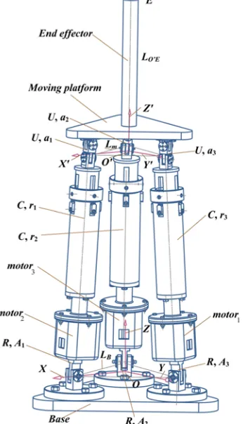
1.2 System Description

Fig. 1.Symmetrical parallel bionic robot leg with three UCR limbs

1.3 Error Model

i i

OA a O O′ and OO EO′ in the 3-UCR parallel manipulator are considered as the closed-loop kinematic chains, and the following equation can express the spatial vector of the drive limbs.

3

i i O iO O O E i

A a =OE+D ′O a′ ′−D ′ L ′ −OA

   

, (4) where the vectors of O a′ _iO′



and O E′ _O′



with reference to the relative coordinate system can be denoted asO a′ _i and O E′ _O′



, respectively. The orientation matrix of the moving platform can be denoted as D_O′ and D_O′3 denotes the third row of it. The vector of O E′ can be described by

[

0 0 L_{O E}′

]

T by analyzing its spatial relation. In the process of error transmission, the nominal numbers are different to the effective displacements of the structure parts. By complete differential calculation to the outputs of the parallel manipulator, the error effects can be fully studied , and Eq. (4) can be expressed as follows:

3 3 0.

i i

i i iO O

O iO O E O O O E i

OE O a

O a L L OA

δ δ δ δ

δ δ δ δ

′ ′

′ ′ ′ ′ ′ ′

′

+ − − −

′

− + + + =

e e D

D D D

   

r r 

r r

(5)

Due to 1

i i

T =

r r

e e

 

and 0

i i

T

δ =

r r

e e , left-multiplied

by

i T

r

e , the Eq. (5) can be simplified as Eq. (6), where δr_i and δOE equal to

[

δr₁ δr₂ δr₃

]

an

d

[

δx_E δy_E δz_E

]

T, respectively. T _O′

i

r

e D



and

O′O a′ iO′

D  equal to

[

T_DI1 T_DI2 T_DI3

]

and

[

1 2 3

]

T

I I I

T T T , respectively, where

i

r

e



denotes the corresponding unified vector of the drive limb s:

i i i

i i i

i

3 3 0.

T T T

O iO O iO

T T T

O E O O O E i

OE O a O a

L L OA

δ

δ

δ

δ

δ

δ

δ

′ ′ ′ ′

′ ′ ′ ′

′ ′

− − − +

+ + + =

e e D e D

e D e D e

     

 r r r 

r r r

r

(6)

1 2 3

4 1 5 2 6 3

0,

i E i E i E

i i i

T

x

T

y

T

z

T

q

T

q

T

q

δ

δ

δ

δ

δ

δ

+

+

+

+

+

+

=

,

i=1, 2, 3. (7)

Substituting the above expressions into Eq. (6), the equation can be rearranged as follows:

In order to solve the six output parameters, a system of six equations should be founded. From Eq. (7), other three simultaneous equations are required. According to the kinematic model based on Quaternions parameters of the parallel manipulator conducted in previous section, three corresponding equations are obtained as follows:

1 2 0 2

2

2 3

m

E O E

L

x = − q q + q q L _′ , (8)

(

2 2

)

1 2 0 1

1 2 4 2

2 3 m

E O E

L

y = − − q + q − q q L _′ , (9)

3 0

q = , (10) where xE and yE denote the coordinates of the point E on the end effector.

By substituting 2 2 2

0= 1 2 3

1 2 3

4 1 5 2 6 3 0,

i E i E i E

i i i

T x T y T z

T q T q T q

δ δ δ

δ δ δ

+ + +

+ + + = , i=4, 5, 6. (11)

Eqs. (7) and (11) can be rearrangeed in matrix form:

11 12 13 14 15 16 17

21 22 23 24 25 26 27

31 32 33 34 35 36 37

41 42 43 44 45 46 1 47

51 52 53 54 55 56 2 57

61 62 63 64 65 66 3 67

E E E

T T T T T T x T

T T T T T T y T

T T T T T T z T

T T T T T T q T

T T T T T T q T

T T T T T T q T

δ δ δ δ δ δ                         =                               

6 23× δ R

=     

T2 E , (12)

whereδE_R denotes the error matrix of kinematic parameters, and can be expressed as follows:

1 1 1

1 1 1 2 2

2 2 2 2 3

3 3 3 3 3

1 2 3 1 23 [ , , , , , , , , , , , , , , , , , , , , , , ]

R O E m O a x O a y O a z

OA x OA y OA z O a x O a y

O a z OA x OA y OA z O a x

T O a y O a z OA x OA y OA z

L L r L L L

L L L r L L

L L L L r L

L L L L L

δ δ δ δ δ δ δ δ δ δ δ δ δ δ δ δ δ δ δ δ δ δ δ δ ′ ′ ′ ′ ′ ′ ′ ′ ′ ′ × = E

, (13)

where δL_{O E}′ and δLm denote the length error of

the end effector and the triangle line error on the moving platform, respectively. δr_i represents the length errors of the drive limbs.

i O a x

L

δ ′ , δLO a y′i

and

i O a z

L

δ _′ denote the coordinate errors of the connectors on the m. Note that these errors are referenced to the absolute coordinate system. Similarly, the coordinate errors of the connectors on the B are represented by

i OA x L δ , i OA y L

δ and

i OA z

L

δ .

The error model of the parallel manipulator describing the relations between errors of kinematic parameters and output parameters can be obtained by the above equations.

1.4 Sensitivity Model

Through establishment of the probability model of the parallel manipulator, the effects on the pose of the end effector caused by the geometrical errors of manufacture and assembly can be studied statistically. According to the error model of the manipulator, Eq. (12) is rewritten as

S R R

δE =TδE , (14) where TR representing the mapping between the pose errors of the end effector and the pose errors of the inputs which denoted as δE_S equals to

-1

T T2.

In order to characterize the standard deviations of the pose errors of the end effector caused by the unified standard deviations of error sources in the parallel manipulator, it should be assumed that all elements in δE_R are independent statistically and the mean of the elements equals zero. According to the error transmission matrix, the mathematical expectation of δE_S is zero. Therefore, the corresponding variance of δE_S can be derived as follows:

(

)

(

2

)

S S

D δE =E δE . (15) Rearranging the Eq. (14) gives:

2 R

23 1

23 23 ₁

1 6

23

1 1 1 6

6

1 6 1

T T

S R R R

R i Ri i

Ri R i Ri R i

i i

R i Ri i

T E

E T E T

T E δ δ δ δ δ δ δ = = = × = _× = =      _{ }  = _  _{ }      

∑

∑

∑

∑

E E T T E

  , (16)

where the i-th error source in δE_R is denoted as

ERi

δ , the element in the sixth row and i-th column of TR is denoted as TR6i. Assume that the elements in δE_R are independent statistically, so one has

23 6

2 2 2

1 1

E

S Rji Ri

i j

T

δ δ

= =

=

∑∑

E . (17)

Substituting Eq. (17) into Eq. (15), the following equation is derived:

(

)

23 6

(

)

2 2

1 1

E

S Rji Ri

i j

D δ T E δ

= =

=

∑∑

E . (18)

So relations between standard deviations of δE_R and δE_S can be formulated as follows:

(

)

23 6

(

)

2 2

1 1

E

S Rji Ri

i j

T

σ δ σ δ

= =

=

∑∑

From the above mathematical analysis, the different poses of the end effector result in the change of the pose errors of outputs. In order to describ fully the standard deviations of δE_R and

S

δE , the estimation standard in the whole workspace between them should be established. Suppose that the volume of the workspace is V, so one has

6 2 1

Ri _V Rji

j

T dv

τ

=

=

_∫

∑

. (20)

The above equation can describe all error sources of the parallel manipulator in its workspace, however, it can't achieve the further sensitivity analysis under the case of specific error compensation and identification. Therefore a novel statistical model of sensitivity coefficients, to implement the unified process on the above error sources in the workspace is presented as:

23

1 Ri Ri

Ri i

τ τ

τ

=

=

∑

. (21)

2 STRUCTURE CALIBRATION

2.1 Calibration Model of Kinematic

Parameters

The mechanical structure of the parallel manipulator is assembled and the kinematic parameters can be identified by the calibration of kinematic parameters. In order to achieve the static mathematical compensation of the manipulator, it is necessary to modify the control model of kinematics according to the identified error parameters.

The pose of the end effector consist of three position parameters and three orientation parameters. In order to solve 23 kinematic parameters in δE_R , it is necessary to measure four groups of the pose by the testing instruments of the end effector in every calibration. According to the kinematic model and its differential form of the parallel manipulator, Eq. (22) can be obtained:

1 2 3 4

T

T T T T

S  S S S S  R R

∆E = ∆_ E ∆E ∆E ∆E _ = ∆J E ,(22)

where [ , , , ₁, ₂, ₃]T

Si xE yE zE q q q

∆E = ∆ ∆ ∆ ∆ ∆ ∆ ,

i=1,2,3,4. A group of the pose error of the end effector is represented as ∆E_Si. J_R, a matrix of 24 rows and 23 columns, denotes the Jacobi

matrix of calibration. The Eq. (22) can be changed as:

(

_T

)

1 _T

R R R R S

−

 

∆ =_{ }∆

 

E J J J E . (23)

Implementing the Eq. (23) gives the iterative value compensating the matrix ER in the course of the kinematic calibration. The kinematic parameters can be calibrated by modifying the iterative value till the errors are less than the terminating value defined in advance. From Eq. (23), the matrix of the pose errors and the Jacobi matrix of calibration is needed to solve the iterative value. The corresponding procedures to obtain the matrixes are shown as follows.

2.2 Analysis of the Pose Errors Matrix

Four groups of the pose of the end effector can be synthesized as the same expression. In order to describe the pose of the end effector, formulating the orientation matrix gives:

0 1

E xyz W

 

= _D E _

E , (24)

where DE and Exyz denote the orientation matrix of the calibrated point and the geometrical vector of the calibrated point, respectively..

By calculating the orientation matrixes based on the measured values and the theoretical values, the matrix of the pose errors is derived as the following equation:

(

)

1

0 1

E xyz

W W WS W

− ∆ ∆ 

∆ = − _{=  }

 

D E

E E E E , (25)

where EW and EWS denote the theoretical values solved by the kinematic model ,and the measured values, respectively. Herein, ∆E_xyz equals to

[ ]T

E E E

x y z

∆ ∆ ∆ .

The error of the orientation matrix

E

∆D can be expressed as:

12 13

21 23

31 32

0 0

0

E E

E E E

E E

D D

D D

D D

∆ ∆

 

 

∆ = ∆_ ∆ _

∆ ∆ 

 

D , (26)

where the expressions of elements in the matrix are the same as the above orientation matrix in the error model.

achieved by substituting the errors of the pose and the Quaternions parameters into Eq. (22).

2.3 Analysis of Calibration Jacobi Matrix

Similar to the analysis of the pose errors, the Jacobi matrix of calibration consist of four submatrixes denoted as JRi. Because of the same expressions of the submatrixes, the analysis of the Jacobi matrix of calibration can be simplified as the analysis of one submatrix, that is:

S Rij

Rij

∂ =

∂ E J

E

,

j=1, 2,23. (27)

According to the analysis of the error sensitivity, different error sources of kinematic parameters with the same error values have different effect on the pose error of the end effector. It is essential to redefine the offset denoted as ∆e_Rij in JRij based on the sensitivity coefficients of the errors for calibrating better the end effector. And the offset can be written as:

Eij Rij

Ri

e e

τ ∆

∆ = , (28)

where∆e_Eijdenotes the j-th offset that need to be calibrated.

By the derivation of the offsets, the Jacobi matrix of calibration can be derived as:

3

1 2

E E E

Rij

Rij Rij Rij Rij Rij Rij

q

x y z q q

e e e e e e

∆ ∆ ∆ ∆ ∆ ∆ 

=  

∆ ∆ ∆ ∆ ∆ ∆

 

 

J .(29)

2.4 Calibration Algorithm of Kinematic Parameters

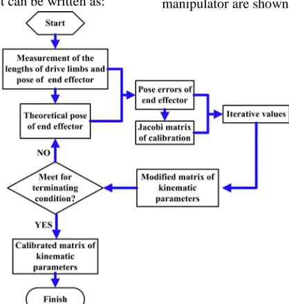
Measuring the practical lengths of the drive limbs and the corresponding pose of the end effector and calculating the theoretical values of the end effector, the kinematic parameters of every joint can be calibrated based on the successive approximation algorithm. The procedures of the calibration algorithm of the manipulator are shown in Fig. 2.

Fig. 2. Calibration algorithm of the kinematic parameters of the parallel manipulator

3 NUMERICAL SIMULATION

3.1 Sensitivity Simulation

Six groups of theoretical values and error values of the parallel manipulator are defined in Table 1.

Table 1. Theoretical values and error values of the parallel manipulator Title Theoretical

value/mm

Error

value/mm Title Theoretical value/mm

Error value/mm r1

Six groups in the

following table 0.05 LO a x′i a1: 0;a2: 25 3;a3: 25 3− 0.08

r2

Six groups in the

r3

Six groups in the

following table 0.05 LO a z′i a1:za1;a2:za2;a3:za3 0.08

LO'E 220 0.1 LOA xi A1: 0;A2: 34 3;A3: 34 3− 0.08

LB 68 3 0.1 LOA xi A1: 68;A2: 34;− A3: 34− 0.08

Lm 50 3 0.1 LOA xi A1: 0;A2: 0;A3: 0 0.08

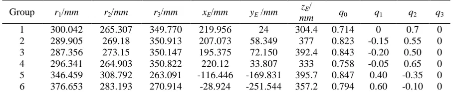
Substituting the theoretical values into the kinematic model, the corresponding

position-orientations of the end effector are obtained and shown in Table 2.

Table 2. Theoretic values of limbs’ lengths and output parameters Group r1/mm r2/mm r3/mm xE/mm yE /mm

zE/

mm q0 q1 q2 q3 1 300.042 265.307 349.770 219.956 24 304.4 0.714 0 0.7 0 2 289.905 269.18 350.913 207.073 58.349 377 0.823 -0.15 0.55 0 3 287.356 273.15 350.147 195.375 72.150 392.4 0.843 -0.20 0.50 0 4 296.341 264.903 350.822 220.12 33.807 333 0.758 -0.05 0.65 0 5 346.459 308.792 263.091 -116.446 -169.831 395.7 0.847 0.40 -0.35 0 6 376.653 283.193 270.914 -28.924 -251.544 357.2 0.794 0.60 -0.10 0

According to the statistical model of sensitivity coefficients, the pose errors of the end effector caused by the errors of kinematic parameters in the whole workspace can be

calculated respectively. Normalizing the results of the above process gives the sensitivity percentages of twenty-three kinematic parameter errors in Eq. (13) shown as Fig. 3.

Fig. 3. Sensitivity percentages of kinematic parameters

From Fig. 3 it is known that the kinematic parameters with symmetrical connectors, such as A2, a2, A3 and a3, have the similar effect on the

pose errors of the end effector and the result validates the sensitivity model by the structure characteristics. Comparatively, the greater sensitivity percentages of the drive limbs represent that the actuator errors have more effect on the pose errors of the end effector. Due to the errors of some kinematic parameters, including

1

OA z

L

δ ,

2

OA z

L

δ and

3

OA z

L

δ , having the greater sensitivity percentages, it is essential to control

The symbol

η

denotes the structure scales which is the ratio of the fix radiuses of the base and the moving platform. The variation of the

sensitivity percentage of the kinematic parameters with different structure scales are given in Fig.4.

Fig. 4. Sensitivity percentage of kinematic parameters with different structure scales

According to Fig. 4, it is known that, with the variation of the structure scale, the sensitivity percentages of kinematic parameters have not been changed obviously in corresponding reachable workspaces. On the other hand, it is necessary to strictly control the kinematic parameters with different structure scales having greater sensitivity percentages.

3.2 Calibration Simulation

For validating the calibration algorithm of kinematic parameters, the iterative calculation of the given kinematic parameters by the numerical simulation is given as follows. The kinematic parameters is shown in Table 1, and the

corresponding errors of these parameters is presented in ∆E_R:

1 23

[ 0.1, 0.1, 0.05, 0.08, 0.08, 0.08, 0.08, 0.08, 0.08, 0.05, 0.08, 0.08, 0.08, 0.08, 0.08, 0.08, 0.05, 0.08, 0.08, 0.08, 0.08, 0.08, 0.08]

R

T

×

∆ = − − −

− − −

− − − −

− E

,

where the errors of kinematic parameters ∆E_R

correspond to Eq. (13).

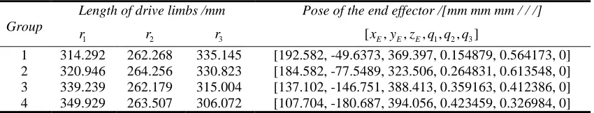
Substituting four groups of the kinematic parameters into the kinematic model of the manipulator, the corresponding poses of the end effector are shown in Table 3.

Table 3 Poses of the end effector with four groups of limbs

Group

Length of drive limbs /mm Pose of the end effector /[mm mm mm / / /]

1

r r2 r3 [xE,yE,zE,q q q1, 2, 3]

1 314.292 262.268 335.145 [192.582, -49.6373, 369.397, 0.154879, 0.564173, 0] 2 320.946 264.256 330.823 [184.582, -77.5489, 323.506, 0.264831, 0.613548, 0] 3 339.239 262.179 315.004 [137.102, -146.751, 388.413, 0.359163, 0.412386, 0] 4 349.929 263.507 306.072 [107.704, -180.687, 394.056, 0.423459, 0.326984, 0]

Taking the lengths of the drive limbs, the poses of the end effector in Table 3 and the values of the kinematic parameters in Table 1 into the kinematic calibration program of the parallel manipulator and calculating iteratively 7 times, the modified matrix of kinematic parameters is obtained. ∆E_Sdenotes the corresponding norm of

the pose errors of the end effector, it is less than the terminating value, defined as 0.01, which has no unit because of having no uniform unit in

S

values and the given errors of the kinematic parameters in the numerical simulation.

The terminating time in the calibration program is decided by the absolute difference of the truth values and the modified kinematic

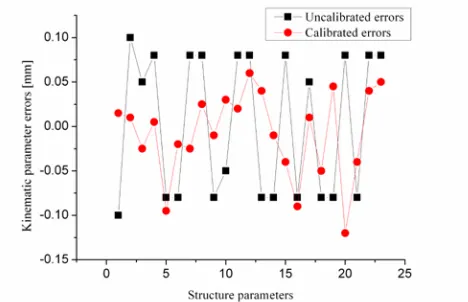
parameters. For the purpose of representing the change of kinematic parameters, the changes of uncalibrated kinematic parameters and calibrated kinematic parameters are shown in Fig. 5.

Fig. 5. Comparison of the uncalibrated kinematic parameters and calibrated kinematic parameters

From Fig. 5 above, it is known that: most errors of calibrated kinematic parameters are decreasing greatly, especially the kinematic parameters with high sensitivity percentage, and the successive approximation algorithm based on the statistical sensitivity coefficients is validated. Because of being lower-mobility parallel manipulator, the errors of kinematic parameters caused by uncontrolled degree-of-freedom cannot be compensated completely. Most errors of kinematic parameters are only less than the terminating value. Contrarily, due to the equilibration effect of least squares method, some errors of calibrated kinematic parameters, such as

1

O a y

L

δ _′ and

3

O a z

L

δ _′ , are increasing. In the course of calibration of kinematic parameters, the sensitivity coefficients and calibrated kinematic parameters with increasing errors have always lower sensitivity percentages partly decide the iterative value. The significance of the sensitivity conversion is emphasized by decreasing effectively the errors of kinematic parameters with higher sensitivity percentages. From the comparison in Fig. 5, the calibration algorithm has relatively fast convergence and concrete directivity when optimizing iteratively and is effective to study the calibration questions.

4 CONCLUSIONS

In this study, by the complete differential-coefficient matrix theory, the error model of the parallel manipulator was established. Then, the statistical model of sensitivity was derived by normalizing all error sources in the reachable workspace. According to the results of sensitivity simulation, the sensitivity percentages of the kinematic parameters vared slightly with the variation of the structure scales. The kinematic parameters with higher sensitivity percentages which should be controlled strictly were distinguished. In the course of manufacture and assembly, decreasing the length errors between the origin in the relative coordinate system and the joint connectors on the base is essential, especially the error decrease along Z-axis perpendicular to the base.

Based on the successive approximation algorithm, the calibration model with sensitivity conversion was established. According to the corresponding simulation, the algorithm is effective to study the calibration question by comparing the values of every kinematic error and has relatively fast convergence when optimizing iteratively. With the conversion according to analytical results of sensitivity coefficients, the operation steps have concrete directivity.

not only of less-DOF but also of six-DOF parallel manipulators. When it is applied to the six-DOF parallel manipulator, all source errors according to six limbs should be considered, and dimensions of corresponding matrixs such as △ER, TR and T2 would change accordingly, but the main analysis steps is the same as the application to the less-DOF parallel manipulators.

5 ACKNOWLEDGEMENTS

This research is supported by the National Natural Science Foundation of China (Grant No. 50905180) and the youth foundation of China University of Mining and Technology (Grant No. OE090191).

6 REFERENCES

[1] Hunt, K.H. (1978). Kinematic geometry of mechanisms. Clarendon Press, Oxford, New York,.

[2] Ryu, D., Song, J.B., Cho, C., Kang Kim, S. M. (2010). Development of a six DOF haptic master for teleoperation of a mobile manipulator. Mechatronics, vol. 20, p. 181-191.

[3] Ropponen, T., Arai, T. (1995). Accuracy analysis of a modified Stewart platform manipulator. IEEE International Conference on Robotics and Automation, vol. 1, p. 521-525.

[4] Wang, J., Masory, O. (1993). On the accuracy of a Stewart platform-Part I: The effect of manufacturing tolerances. IEEE International Conference on Robotics and Automation, vol. 1, p. 114-120.

[5] Huang, T., Li, Y., Tang, G., Li, S., Zhao, X. (2002). Error modeling, sensitivity analysis and assembly process of a class of 3-DOF parallel kinematic machines with parallelogram struts. Science in China: Series E, vol. 45, no. 5, p. 467-476.

[6] Alici, G., Shirinzadeh, B. (2006). Optimum dynamic balancing of planar parallel manipulators based on sensitivity analysis. Mechanism and Machine Theory, vol. 41, p. 1520-1532.

[7] Pott, A., Kecskeméthy, A., Hiller, M. (2007). A simplified force-based method for the linearization and sensitivity analysis of

complex manipulation systems. Mechanism and Machine Theory, vol. 42, p. 1445-1461. [8] Binaud, N. (2010). Sensitivity comparison of

planar parallel manipulators. Mechanism and Machine Theory, vol. 45, no. 11, p. 1477-1490.

[9] Merlet, J.P. (2006). Parallel Roberts. Springer, Dordrecht.

[10] Cedilnik, M., Soković, M., Jurkovič, J. (2006). Calibration and Checking the Geometrical Accuracy of a CNC Machine-Tool. Strojniški vestnik - Journal of Mechanical Engineering, vol. 52, no. 11, p.752-762.

[11] Zhuang, H., Masory, O., Yan, J. (1995). Kinematic calibration of a stewart platform using pose measurement obtained by a single theodolite. IEEE International Conference on Intelligent Robots and Systems, p. 329-334.

[12] Daney D. (2003). Kinematic calibration of the Gough platform. Robotica, vol. 21, no. 6, p. 677-690.

[13] Papa, G., Torkar, D. (2009). Visual Control of an Industrial Robot Manipulator:Accuracy Estimation. Strojniški vestnik - Journal of Mechanical Engineering, vol. 55, no. 12, p.781-787.

[14] Khalil, W., Besnard, S. (1999). Self calibration of Stewart-Gough parallel robot without extra sensors. IEEE Trans. On Robotics and Automation, vol. 15, no. 6, p. 1116-1121.

[15] Chiu, Y., Perng, M. (2004). Self-calibration of a general hexapod manipulator with enhanced precision in 5-DOF motions. Mechanism and Machine Theory, vol. 39, p. 1-23.

[16] Zhang, Y., Cong, S., Li, Z., Jiang, S. (2007). Auto-calibration of a redundant parallel manipulator based on the projected tracking error. Archive of Applied Mechanics, vol. 77, p. 697-706.

[17] Jeong, J., Kim, S., Kwak, Y. (1999). Kinematics and workspace analysis of a parallel wire mechanism for measuring a robot pose. Mechanism and Machine Theory, vol. 34, p. 825-841.

Journal of Machine tools & Manufacture, vol. 43, p. 1051-1066.

[19] Hart, J.C., Francis, G.K., Kauffman, L.H. (1994). Visualizing quaternion rotation. ACM Transactions on Graphics, vol. 13, no. 3, p. 256-276

.

[20] Senan, N.A.F., O’Reilly, O.M. (2009). On the use of quaternions and Euler–Rodrigues symmetric parameters with moments and moment potentials. International Journal of

Engineering Science, vol. 47, no. 4, p. 599-609.

[21] Arribas, M., Elipe, A., Palacios, M. (2006). Quaternion and the rotation of a rigid body. Celestial Mechanics and Dynamical Astronomy, vol. 96, no. 3-4, p. 239-251. [22] Cayley, A. (1843). On the motion of rotation