DESERT 15 (2010) 33-43
Determining the effect of physical characteristics on flood
hydrograph
(Case study: Western section of Jazmurian Basin)
A. Salajegheh
a, S. Dalfardi
b*, M. Mahdavi
c, A. Bahremand
d, A. Afzali
ea
Associate Professor, Faculty of Natural Resources, University of Tehran,Karaj, Iran
b
Lecturer, Islamic Azad University of Jiroft, Jiroft, Iran
c
Professor,Faculty of Natural Resource, University of Tehran, Karaj, Iran
d
Assistant Professor, Gorgan University of Agricultural Sciences and Natural Resources, Gorgan, Iran
e
Senior Expert, International Desert Research Center, University of Tehran, Semnan, Iran
Received: 6 February 2009; Received in revised form: 25 November 2009; Accepted: 1 January 2010
Abstract
Flood causes great and uncompressible damage to people’s life and properties as well as environment each year in Iran. This research was carried out at the west section of Jazmurian basin that placed in the southeast of Iran. In this research physical characteristics such as area (A), perimeter (Pr), average elevation of basin (av.e), average slope (av.s), gravelious coefficient (G), length of main stream(L), pure slope of main stream(Pur), Lc, Tc and Tl for independent variables and hydrograph component such as Qp, Q25, Q50, Q75, Tp, T25, T50, T75 and Tb for dependent variables were used. For this the data of 12 hydrometric stations were used. Normality test was done by kolmograph- Smironov. After that using two and multiple variables regression analysis and with the use of modeling, the relation between dependent and independent variables were defined. The evaluation of hydrologic model behavior and Performance is commonly made and reported through comparisons of simulated and observed variables. Frequently, Comparisons are made between simulated and measured stream flow at the catchments outlet. Significant models are included the models that have correlation coefficient bigger than 0.325 at 1 percentage level and bigger than 0.250 at 5 percentage levels. We used three criteria such as RMSE, RE and CE for selecting the ultimate models. These models have less RMSE and RE and more CE .The results approve that with the use of physical characteristics of the basin we can determine the synthetic hydrograph. The results also show that the two- variable models have higher efficiency in estimating the discharge variables of the simulated hydrographs.
Keywords: Physical attributes; Hydrological modeling; Synthetic hydrograph; Dependent variable; Jazmurian basin; Iran
1. Introduction
The fact that the world faces water crises has become increasingly clear in recent years. Challenges remain widespread and reflect severe problems in the management of water resources in many parts of the world. These problems will intensify unless effective and concerted actions are taken”(WWAP, 2003). For appropriate design of hydraulic structures
Corresponding author. Tel.: +98 913 248 8529,
Fax: +98 261 2227765.
E-mail address:[email protected]
And flood control structures, information must be known about the hydrology of the system, such as peak discharge, runoff volume, and the time
using frequency analysis of flood (Afshar 1990). Providing flood properties at the watersheds without statistical Data is very hard. Empirical formulas, Synthetic hydrograph, simulation methods, statistical estimation of maximum instantaneous are analyzed and flood indicator are used for supplying maximum of instantaneous flood in those watersheds without hydrometric station. Among these methods, some which result in simulating hydrograph are able to describe the exact details of flood (compolar & solodati, 1999). In other words important necessary properties of flood can be derived after determining the flood hydrograph. But most of the time because of hydrographs limitations, the design flood hydrograph is obtained by another way for applications (Afshar, 1990). We need to have discharge data as time series to illustrate hydrographs, since there are no enough discharge information and hydrometric stations and also because of the good mathematical relationships between catchment characteristics and hydrograph properties and components, we try to develop the synthetic hydrographs using the mentioned relationships. Dooge (1977) comments that many of first models were based on empirical equations developed under unique conditions and used in applications with similar conditions. An urgent need in hydrology is to apply models to predict in ungauged basins and hence traditional calibration of models is not possible (Sivapalan et al., 2003).Hydrological models are primarily predictive models, meaning they obtain a specific answer to a specific problem. Other models are developed to be investigative, meaning they increase our understanding of hydrological processes (O’Connell, 1991). There are many proposed models to calculate of synthetic hydrograph, they used for special condition and could not be used in different location (Afshar, 1995). The models are suitable instrument for decision making in hydrologic affairs and for developing these models doing accurate and effective watershed's assessment is necessary (Deal et al. 2008). Efficiency criteria are defined as mathematical measures of how well a model simulation fits the available observations (Beven, 2001). Models simplify the system and simulate watershed behaviors and represent the relations existed between the characteristics of basin and their hydrograph response. There for studying the affairs that take place in watershed and estimating its important outputs of it such as flood and sediment are of
most important duties of watershed manager (Telvari 1996). There for hydrologic modeling provided by physical attributes can solve many of problems in relation with hydrologic studies. Because different location in our country are under risk of frequent floods, there for developing these models is very high value and with use of these models we can save our different natural and humanity resources.
2. Materials and methods
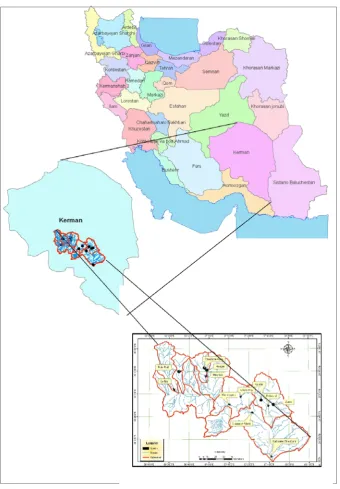
The Jazmurian watershed is located at southeast of Iran and is surrounded by Bazman, Jabalbarez, Hazar and Lalehzar mountains. It is bounded on the south by Bashagard Mountains. All of rivers and streams in this watershed are inflowing toward plain of Jazmoran. It's located between 56˚, 15΄ until 61˚, 23΄ east longitude and 26˚, 28́ until 29˚, 30́ north latitude. Its area is 69621 Km2 of which about 32459 Km2 is area
of plains and fans, and 3000 Km2 saltish area,
wetlands and swamps. This research was carried out in northwest part of Jazmurian where the mountains are, and the main stream and rivers of the basin with an important role on flooding are located in this part. Baft and Esfandaghe plains are located at the farthest end of northwest of jazmurian watershed with high elevation. There are three cities including Jiroft, Baft and Iranshahr are located in this watershed. The required information for this research includes 10 physical characteristics (Independent variables) and component of flood hydrograph (dependent variables). the information concerning flood hydrograph is obtained from Water Recourses Research Institute of Iran (TAMAB) and also Kerman's water department and physical characteristics are obtained from digitized topographic maps with scale of 1/50000 ( sheets related to west section of Jazmurian ).
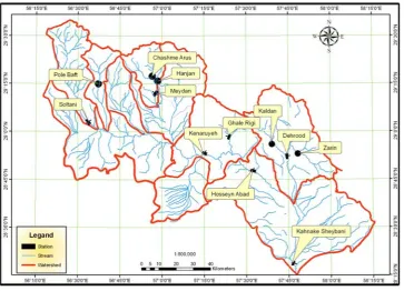
12 hydrometric stations were selected at the studied location (Table 1). After collecting required information of to mentioned stations from related departments, hydrographs designed on coordinate axis and Hawk Belly hydrographs were selected.
Fig. 1. Situation of the studied watershed
Table 1. Hydrometric stations in the studied watershed
No. Name of station River Area (km^2)
1 Soltani Soltani 935
2 Koldan Rabor 191
3 Ghale rigi Ramon 249
4 Konaroie Halil rood 7600
5 Zarin Saghder 330
6 Dehrod Shor 1361
7 Hosein abad Halil rood 8420
8 Meydan Seyed morteza 520
9 Hanjan Rodar 311.2
10 Pole Baft Baft 261
11 Chashme Aroos Rabor 100.4
Fig. 2. Location of hydrometric stations in the study area
Peak discharge, base time, discharges of 25%, 50% and75% of the peak, time to peak, the times corresponded to discharge of 25%, 50% and 75% that are important component of hydrograph (Snyder 1938 & Gupta et al, 1986) were selected for developing hydrologic models. These variables were extracted from available hydrographs. Hydrographs were plotted on coordinate system and then dependent variables were extracted. Hygrograph’s component as dependent variable and physical attributes as independent variables were used for modeling and providing synthetic hydrograph by soft ware SPSS.
Two and multiple regression, were used to determine relationships between dependent and independent variables with the intention of determination and assessment of main factors controlling hydrograph components and also homogeneity of accepted stations. SPSS 13 software was applied for statistical analysis (Esmailian, 2002). Regarding to degree of freedom (n-2), the models which its correlation coefficient were equal or more than 0.250 and 0.325 in 1% and 5% level respectively were significant models (Mahdavi, 2002). The Colmograph- smironov test was used for normality of data. Also homogeneity test for variance of error were used by plotting values of standard error against values of standardized prediction. The accepted points were tested for being monotonous and uniform, and no self correlation test between errors was done using
Durbin – Watson test with acceptable values near 2. Also analysis of outliers by use of casewise diagnostics test and occurrence of studied values was done within a range of 3 times of standard deviation (Mozayan, 2003). The regression models were indeed developed from finding direct relations among variables or their changed forms.
Therefore pair relations between variables in states of linear , logarithmic , inverse ,two degree , three degree , complex, power, s curve , growth curve and exponential were studied and suitable models related to each of these state were selected (mozayan, 2003). To determine linear relation between dependent and independent variables, polygonal linear relation test was used (Affifi and Clark, 1995) involving one formula containing relation between one of depended variables with all of independent variables.
estimation and approval (RE), residual mean square error (RMSE) and finally coefficient efficiency (CE) were used (Formula 1-3).
100 Yo Y Yo RE e n Y Y RMSE i e o
1 1 2 ) ( ) ( 1 ) ( 1 ) ( 1 1 2 1 2 1
o o i n e o i n o o i n E Q Q n Q Q n Q Q nC
(1-3)
Where in this formula RE= relative error in percentage, RMSE=residual mean square error, Ye=estimated value of dependent variable, Yo=observed value of dependent variable, n=the number of variable, Qo= observed value of discharge, Qe= estimated value of discharge,
o
Q =mean observed value of discharge. Final selection of extracted models were accomplished by less relative error of estimation and approval and residual mean square error and more coefficient efficiency and adjusted coefficient of determination.
3. Results
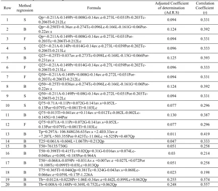
Determination of the best relationship between hydrograph components and physical characteristics of watershed is the main objective of this research. With these relationships, the hydrograph components can be calculated using physical characteristics of the catchment. For achieving this objective after determining dependent and independent variables the relationships between these variables were determined by two and multiple variable regression. Evidently in equal condition, the models with more adjusted coefficient of determination, less estimation and approval error and less number of independent variables were selected as the best models. Multiple variable regressions, linear and nonlinear models were extracted using spss
(tables 2 and 3). In each table the formulas accompanied by adjusted coefficient of determination and correlation coefficient were given. Based on the correlation coefficient, the significant or not significant models were distinguished. Adjusted coefficient of determination showed that how many percentages of dependent variables were explained by independent variabls. As it can be seen from the tables, the discharges components with time components have bigger adjusted coefficient of determination in terms of meaningful significance, therefore they were better for modeling purpose. From statistical point, the two-variable regression showed to be better than other methods, based on its high adjusting coefficient of determination. The ultimate models were chosen from two variable models with higher efficiency coefficient. With attention to adjusted coefficient of determination in two variable regressions (table 2) it was observed that in formula with more adjusted coefficient of determination, two independent variables including area and perimeter are the most effective for explanation of dependent variables. in linear regression models the adjusted coefficient of determination equal to 0.018 and correlation coefficient equal to 0.26 has the lowest adjusted coefficient of determination that is for T25 (model no.9) and opposite of it the adjusted coefficient of determination equal to 0.135 and correlation coefficient equal to 0.387 has the highest adjusted coefficient of determination that is for Q25 (the model No.47).
Table 3 shows the result of linear regression from this table it shown that exception of models No.19 and No.20 connected with Tb , the models connected with discharge related to time has more adjusted coefficient of determination which it correspond to result of non curve linear regression. Three method of stepwise, backward and forward were used by linear regression that back ward was more significant. The lowest r2 is for Tp (model
No.13) and the highest r2 for Tb (model No.19).
In linear regression also discharge component has more adjusted R2 relative to the time
Table 2. Result of prevalent two variable regression models
Correlation Coefficient (r) Adjusted Coefficient of
determination (Ad.R.S) Formula Row 0.306 0.046 Tp=150.466+(0.207A)+(-4.3E-0.005A2)+(2.14E-0.009A3) 1 0.260 0.027 T50=e(3.985+(-1053/lc)) 2 0.337 0.067 Tb=29.164+(0.006A)+(-106E-0.006A2)+(9.11E-0.011A3) 3 0.309 0.048 Tp=-13.904+(4.068Pr)+(-0.014Pr2)+(1.27E-0.005Pr3) 4 0.276 0.028 T25=-29.778+(1.937Pr)+(-0.007Pr2)+(0.06E-0.006PR3) 5 0.337 0.067 Tb=22.3+(0.167Pr)+(-0.001Pr2)+(6.88E-0.007Pr3) 6 0.258 0.051 T50=-77511.3+76125.73G 7 0.247 0.045 T75= e(5.12+(-4.053/lc)) 8 0.26 0.018 T25=-73.747+(156.872av.s)+(-34.771av.s2)+(2.174av.s3) 9 0.252 0.019 T25=e(3.479+(-1E+0.033/av.e)) 10 0.335 0.065 TP=-29.933+(12.616L)+(-0.11L2)+0 11 0.274 0.027 T25=-29.571+(5.454L)+(-0.045L2)+0 12 0.340 0.069 Tb=20.3+(0.567L)+(-0.006L2)+(1.58E-0.005L3) 13 0.347 0.074 TP=-31.204+(108.137Tc)+(-7.927Tc2)+(0.145Tc3) 14 0.272 0.025
T25=-27. 545+(46.087Tc)+(-3. 358Tc2)+(0.061Tc3) 15 0.249 0.046 T50=23573. 344+3173.918Tc 16 0.236 0.04 T75=3358.087+40192.748log(Tc) 17 0.332 0.064 Tb=22.129+(3.991Tc)+(-3. 36Tc2)+(0.007Tc3) 18 0.348 0.075 Tp=-42. 329+(187.349Tl)+(-23.428Tl2)+(0.752Tl3) 19 0.275 0.027
Table 3. Result of prevalent linear regression models Correlation Coefficient (r) Adjusted Coefficient of determination (Ad.R.S) Formula Method regression Row 0.331 0.094 Qp=-0.211A-0.149Pr+0.008G-0.14av.e-0.273L+0.031Pr-0.203Tc-0.206Tl-0.212Lc S 1 0.392 0.124 Qp=-0.250Tl+0.36av.e-0.274Tc-0.096Lc-0.166L-0.161G+0.06Por-0.22av.s B 2 0.331 0.094 Qp=-0.211A-0.149Pr+0.008G-0.14av.e-0.273L+0.031Por-0.203Tc+0.206Tl-0.212Lc F 3 0.333 0.096 Q25=-0.21A-0.14Pr+0.014G-0.14av.e-0.273L+0.039Por-0.202Tc-0.206Tl-0.213Lc S 4 0.393 0.125 Q25=-0.25Tl+0.037av.e-0.273Tc-0.098Lc-0.168L-0.15G+0.066Por-0.231av.s B 5 0.333 0.096 Q25=-0.21A-0.149Pr+0.014G-0.14av.e-0.27L+0.039Por-0.202Tc-0.206Tl-0.213Lc F 6 0.331 0.094 ً Q50=-0.211A-0.149Pr+0.008G-0.14av.e-0.272L+0.031Por-0.203Tc-0.206Tl-0.212Lc F 7 0.392 0.124 Q50=-0.25Tl+0.036av.e-0.274Tc-0.096Lc-0.166L-0.161G+0.06Por-0.22av.s B 8 0.331 0.094 Q50=-0.211A-0.149Pr+0.08G-0.14av.e-0.272L+0.031Por-0.203Tc-0.206Tl-0.212Lc S 9 0.296 0.077 ً Q75=0.71A+0.11Pr+0.072G-0.141av.s+0.052L-0.13Por+0.079Tc+0.081Tl+0.103Lc S 10 0.387 0.130 Q75=0.013Tl+0.041av.e+0.114av.s+0.012Tc-0.082L-0.002Lc-0.145G+0.144Por B 11 0.296 0.077 Q75=0.071A+0.11Pr+0.072G-0.141av.s+0.052L-0.13Por+0.079Tc+0.081Tl+0.103Lc F 12 0.419 0.011
Tp=0.297A- 106.848G36.635av.s +2.4E0.33av.e +7.207L+503.355Por-9.423Tc-11.06Lc +6.525Pr+0.487Qp B 13 0.333 0.047 T25=0.061A+0.604L+1.067Pr+0.212Qp B 14 0.258 0.051 T50=76135/730G B 15 0.214 0.03 T50=0.398Tl+0.415Tc+0.02Qp+0.31G-0.016av.s+0.074Lc-0.048av.e+0.09L+0.185Por-0.964A B 16 0.258 0.051
T50=-0.068A-0.059Pr +0.031Av.s +0.007av.e +0.027L+0.072Por +0.108Tc+0.099Tl+0.03Lc+0.013Qp B 17 0.198 0.023 T75=0.365Tl+0.046Qp+0.381Tc+0.324G-0.043av.s+0.068Lc-0.066av.e+0.059L+0.17P-1.226A B 18 0.574 0.255 Tb=-0.012A+0.0228Pr+1.06E-0.34av.e+0.442L-0.899Lc+0.062Qp B 19 0.557 0.248 Tb=0.008A+0.148Pr+0.369L-0.752Lc+0.062Qp B 20
The criteria of the coefficient efficiency (most important) (CE) , relative error (RE) and residual mean square error ( RMSE) were used for selection of ultimately models that relative to other models included more CE and less
RMSE and RE. For purpose of statistical for each dependent variable only one model that was the best statistical model (have more CE and less RE and RMSE) were selected (Table 4).
Table 4. ultimate regression models for estimation of hydrograph, s component
Row Dependent variable Formula
Correlation Coefficient (r) Adjusted Coefficient of determination (Ad.R.S) Coefficient efficiency (CE) Residual mean square error (RMSE) Relative error (RE)
1 Qp Qp=e(4.28+(-77.694/Pr)) 0.37 0.123 0.259 62.52 0.128
2 Q75 Q75=e(3.992+(-77.643/pr)) 0. 37 0.122 0.259 62.54 0.128
3 Q50 Q50=e(3.587+(-77.691/Pr)) 0.37 0.123 0.259 62.54 0.128
4 Q25 Q25=e(2.89+(-77.608/Pr)) 0.371 0.123 0.252 62.42 0.124
5 Tp Tp=e(5.517+(-5.053/Lc)) 0.269 0.056 1.05 33.52 0.004
6 T75 T75=e(5.12+(-4.053/Lc)) 0.247 0.045 1.50 27.03 0.27
7 T50 T50=e(3.985+(-1.054/Lc)) 0.260 0.027 1.03 29.06 0.29
8 T25 T25=e(3.479+ (-1E+0.033/av.e)) 0.252 0.022 0.852 23.284 0.07
9 Tb Tb=21.598+(7.027Tl)+ (1.012Tl2)+(0.035Tl3) 0.333 0.064 0.954 23.29 0.01
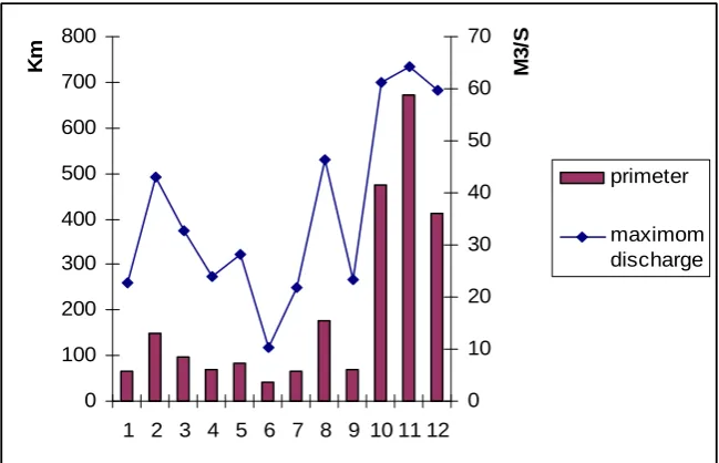
Figure 3 shows relation of estimated maximum discharge by connected model with perimeter of different stations in studied
0 100 200 300 400 500 600 700 800
1 2 3 4 5 6 7 8 9 10 11 12
Km
0 10 20 30 40 50 60 70
M3
/S
primeter
maximom discharge
Fig. 3. Relation of perimeter with estimated maximum discharge
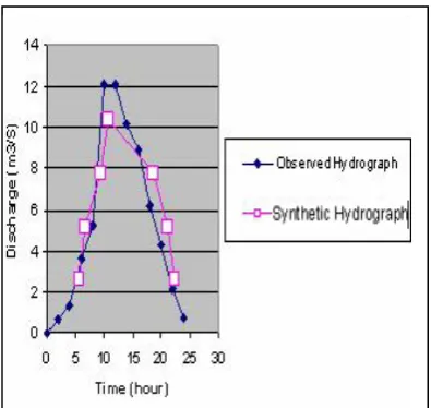
Graphic method was used for assessment extracted models by drawing observed hydrographs against synthetic hydrographs. Observed hydrograph were extracted by taking average of hydrographs for different stations. Rising limb of synthetic hydrographs were extracted by using models of Table 4 and Falling limb of synthetic hydrograph (rising and falling limb have the constant slope) were extracted by Snyder method. Comparing and assessment of observed and synthetic hydrograph were showed in figures 4-13.
Fig. 4. observed and estimated hydrograph For to Soltani station
Fig. 5. observed and estimated hydrograph for to Dehrood station
Fig. 7. observed and estimated hydrograph for to Koldan station
Fig. 8. observed and estimated hydrograph for to Zarin station
Fig. 9. observed and estimated hydrograph for to Hanjan station
Fig. 10. observed and estimated hydrograph for to Chashme Aroos station
Fig. 11. observed and estimated hydrograph for to Ghale Rigi station
Fig. 13. observed and estimated hydrograph for to Konaroie station
4. Discussion and conclusion
Making models in this watershed beacuse of special situation, unsuitable dispersion and low rainfall consequently different discharge, unsuitable dispersion of station and the most important lowing hydrographs related to other location of the country with better condition is relatively hard. Results show Because of lowing variable and quensequently reducing inner relationship and range variable and using one variable for estimation dependent variable, for purpose of statistical, two variable regressions is better than multiple regressions (table 2 and 3). In addition unlinear relation some of two and several variable models for explanation of physical attribute of hydrograph were approval. In which it's correspond to Singh (1992) based on unlinear relation of hydrological variable. Totally extracted results based on simulation hydrograph by physical attributes are correspond to most of last research (such as guptaetal 1986, yen 1997, kalian etal 2003) although estimating variables different component of hydrograph maybe were different. Results of this research based on significant role perimeter and area on controlling maximum discharge of hydrograph is correspond to results of Fuller and Dicken based on following maximum discharge from watersheds area . The results of accomplished research in some area of our country (Nekoimehr 1995, and Dindar hasso, 2000) also denote unability Snyder model in rehabilitation hydrograph and naturally inefficiency of accepted variables in mentioned method. on the other hand it can be deduced by doing analyzed with use of standardized regression coefficient connected to
physical effective factors of watershed in multiple variable formula (table 3) that almost perimeter of watershed have the most controlling role on variable included: Q25, Q50, Q75. Area, gravelious coefficient, medium slope of watershed and LC are next controlling factors of mentioned variable.
Also it deduced by results of higher two variable regression formula in table 3 that time factors of hydrograph in studied watershed is controlled by LC and lag time . in addition intentional and unintentional errors of flood hydrograph have high effect on accomplished works and produced unhomogenity condition and unsuitable correlation between dependent and independent variable in which have to taked into consideration.
Different between extracted results and former result denoted necessity of location studies and consideration controlling variables of hydrograph component. by use of extracted results adding up that in spite of very low flood hydrograph for hydrologic analyzing due to scattering data , unmanagment information and also intricacy of governor condition , modeling by ten factors Included area, perimeter , mean elevation , mean slope, lengths of main stream, streams pure slope, gravelious coefficient, concentration time, lag time and LC can be accomplished. Totally it is resulted that possibility of modeling in this watershed and similar areas because of very irregular and unsuitable dispersion rainfall and unhomogenity of location condition related to more damped and with regular rainfall is harder. It should be have more stations and enough frequency of stations for better conditions of modeling.
References
Affifi, A.A. and Clark, V., 1984. Computer - aided multivariate analysis. Life time Learning Publications Belmont, California, 45pp.
Afshar, A, 1990, Engineering hydrology, Center publication of collegiate 459 pp.
Campolor, M.A. and Solodati, A., 1999. River flood forecasting with a neural network model. Water Resource Research, 35: 1191-1197.
Dindar haso, A, 2000, calibration of geomorphologic momentarily unit hydrograph of Lighvan, s watershed, thesis submitted to MS.c degree of irrigation, Tarbiat Modares University, 175 pp. Dooge, J.C.I. 1977. Problems and methods of rainfall- runoff modeling. In Mathematical Methods for Surface Water Hydrology. Eds. Ciriani, T.A., Maione, U., and Wallis, J.R. Chichester: Wiley. pp. 71-108.
Publications of the European Communities, Luxembourg.
Esmailian, M, 2004, Education book of SPSS12, one volume, Publication of Naghos, 599 pp.
Jamab consulting engineering company, 1998, water comprehensive design, Grammarian watershed. Gupta, V.K., Waymire, E. and Roddriguez-Iturbo, I., 1986. On scales gravity and network structure in basin runoff. In: Scale Problems in Hydrology. Gupta, V., Rodriguez- Iturbo. I. and Wood. E. (Eds). Holland, 1986: 159-180.
Hashemi, A, 1996, inspecting relation of flood mean discharge with some of physical attribute of watershed (case study Semnan province), thesis submitted to MS.c degree of university of Tehran, 92 pp.
Kalina,L.,Govindarajua, R.S. and Hantushb, M.M., 2003. Effect of geomorphology resolution on modeling of runoff hydrograph and sediment graph over small watershed. Journal of Hydrology, 276: 89- 111.
Mahdavi, M, 2002, applied hydrology, two volumes, fourths edition, publication of University of Tehran, 427 pp.
Mozayan, M, 2003, inspecting relation between different component of rain fall and run off in Kasilian watershed, thesis submitted to MS.c degree, tarbiat modares university , 81pp.
Nekoi mehr, M, 1995, inspecting usage of unit hydrograph with different times in analyzing Zayanderood dam's watershed floods (Plasjan sub basin), Tarbiat Modares University, thesis submitted to MS.c degree, 266 pp.
O’Connell, P.E. 1991. A historical perspective. In Recent Advances in the Modeling of Hydrologic Systems. Kluwer, Dordrecht. pp. 3-30.
Rahimian, R, 1995, inspecting different models of geomorphologic momentarily unit hydrograph and usage it's for making hydrograph in watershed
without statistical data, thesis submitted to MS.c degree of geology, Shiraz University, 101 pp
Rostam afshar, N, 1995, Water recourses engineering, Water recourses research institute (TAMAB), 296 pp. Singh, V.P., 1992, Elementary hydrology. Eastern Economy Edition, New Delhi, India, 973p.
Singh, V.P. 1995. Watershed Modeling. In Computer Models of Watershed Hydrology. Ed. Singh, V.P. Colorado: Water Resources Publications. pp. 1-22. Sivapalan M,Takeuchi K, Franks, SGupta V,KarambiriH,Lakshmi V,Liang X, McDonnell J, Mendiondo E, O,Connell P, Oki T, Pomeroy JW, Schertzer D, Uhlen brook S,Zehe E.2003. IAHS decade on predictions in ungauged basins (PUB), 2003: shaping an exciting future for the hydrological science .hydrological sciences journal 48:892-898. Snyder.F.F., 1938. Synthetic unit-Hydrographs, Transactions of American Geophysics Union 19: 447- 454.
Surkan, A.J., 1969. Synthetics hydrograph: effects of network hydrology, Water Resource Research, 5: 112-128.
Woonsup Choiand Brian M. Deal, 2008. Assessing hydrological impact of potential land use change through hydrological and land use change modeling for the Kishwaukee River basin (USA) Journal of Environmental Management , Pages 1119-1130. WWAP, 2003. Water for People, Water for Life. UN World Water Development Report. Prepared as a collaborative effort of 23 UN agencies and convention secretariats co-ordinated by the World Water AssessmentProgramme. UNESCO, Paris. Yen, B.C. and Lee, K.T., 1997. Unit hydrograph derivation for ungauged watersheds by stream-order laws, Journal of Hydrology, 2(1): 1-9.