Positivity-preserving nonstandard finite difference schemes for
sim-ulation of advection-diffusion reaction equations
M. Mehdizadeh Khalsaraei
Faculty of Mathematical Science, University of Maragheh, Maragheh, Iran
E-mail:[email protected]
R. Shokri Jahandizi
Faculty of Mathematical Science, University of Maragheh, Maragheh, Iran
E-mail:[email protected]
Abstract Systems in which reaction terms are coupled to diffusion and advection transports
arise in a wide range of chemical engineering applications, physics, biology and environmental. In these cases, the components of the unknown can denote con-centrations or population sizes which represent quantities and they need to remain positive. Classical finite difference schemes may produce numerical drawbacks such as spurious oscillations and negative solutions because of truncation errors and may then become unstable. We propose a new scheme that guarantees a smooth numeri-cal solution, free of spurious oscillations and satisfies the positivity requirement, as is demanded for the advection-diffusion reaction equations. The method is applicable to both advection and diffusion dominated problems. We give some examples from different applications.
Keywords. Nonstandard finite differences, Positivity, Advection-diffusion reaction equation, M-matrix.
2010 Mathematics Subject Classification. 65Nxx, 65L12, 65L20, 65M20.
1. Introduction
When one solves differential equations, modeling physical or biological phenomena, it is of great importance to take physical constraints into account. More precisely, numerical schemes have to be designed such that discrete solutions satisfy the same constraints as exact solutions such as positivity, monotonicity and total variation di-mensioning, see for examples [3,6,7,10,11,20]. Numerical schemes are not usually constructed to satisfy those properties explicitly.
Parabolic equations with or without reaction terms are used extensively in the modeling of many physical and biological phenomena such as heat transfer, transport
Received: 1 February 2015 ; Accepted: 23 June 2015.
and reaction of chemical species and population density in mathematical biology. They constitute a central component in applied mathematics and their numerical simulations are fundamental importance in gaining the correct qualitative and quan-titative information on the systems. Since the quantities that are being modeled, concentrations of chemical species and populations sizes are necessarily positive, it is important to have numerical schemes that preserve the positivity of the solution. Numerical methods based on standard finite difference (SFD) or finite element dis-cretizations are widely used, see for example [3,21]. They do not explicitly incorporate the requirement that the solutions be positive. Even though these schemes guarantee convergence of the discrete solution to the exact one, but some times occurs that the essential qualitative properties such as positivity and monotonicity of the solutions are not transferred to the numerical solution. One way of avoiding this disadvantage is to imply finite difference schemes that are nonstandard in the sense of Mickens’ definition [13].
Nonstandard finite differences methods (NSFDs) in addition to the usual prop-erties of consistency, stability and hence convergence, produce numerical solutions which also exhibit essential properties of solutions [2,8,9,12,14–17]. In this paper we propose a new class of NSFD schemes for advection-diffusion-reaction equations by using nonlocal approximation of reaction term. The proposed scheme enable us to solve accurately the examined problems. An important factor for new method is the
positivity preservation of the solution which exhibit essential property of solutions. The rest of the paper is organized as follows: In Section 2, we propose the new method and investigate the positivity and stability requirements. In Section 3, we apply the method to three problems and compared with SFD schemes. Finally we end the paper with some conclusions in Section 4.
2. Scheme construction
The relevant partial differential equation in this study is given as follows
∂C(x, t)
∂t +P
∂C(x, t)
∂x −Q
∂2C(x, t)
∂x2 =−RC(x, t), (x, t)∈[0, xmax]×[0, T], (2.1)
for the unknownC =C(x, t), with appropriate boundary and initial conditions and where the parametersP,Qand Rare positive constants.
Take a partition of the interval [0, xmax], x0 < x1 < · · · < xN with xj = j∆x,
approximation toC(xj, tn). Herej andnare positive integers.
Making use of the nonstandard discretization of the reaction termRC(x, t) in (2.1), it is now desired to find an accurate NSFD scheme which is positivity preserving and can be written as
C(x, t) =a(Cj+1n+1+Cjn+1−1) + ( 1
2 −a)(C n
j+1+Cjn−1), (2.2)
where a is arbitrary parameter to be determined below. The corresponding finite difference approximation provides the equation difference
P Cn+1=N Cn, (2.3)
whereP and N are the following tridiagonal matrices
P=tridiag
−2∆Px−∆Qx2 +aR; 1 ∆t+
2Q
∆x2;
P
2∆x− Q
∆x2 +aR
, (2.4)
N=tridiag
−(1 2 −a)R;
1 ∆t;−(
1 2 −a)R
. (2.5)
The parameterais chosen according to the following theorem.
Theorem 1. If 12 ≤ a ≤ Q
∆x2−2∆Px
R , then the scheme (2.3) is unconditionally pos-itive.
Proof. From (2.3) it is enough to show thatP−1>0 andN ≥0.
• Since,P is an M-matrix, see [23], then we have to put
−2∆Px−∆Qx2 +aR≤0, (2.6)
P
2∆x− Q
∆x2+aR≤0, (2.7)
andP−1>0, see [1]. From (2.6) we can write
a≤
Q ∆x2 +
P 2∆x
R , (2.8)
and From (2.7) we can write
a≤
Q ∆x2 −
P 2∆x
R . (2.9)
• In order to nonnegativity forN, we write
−(1
2−a)R≥0 then a≥ 1
Then, from (2.8), (2.9) and (2.10) we have
1 2 ≤a≤
Q ∆x2 −
P 2∆x
R , (2.11)
and this completes the proof.
Theorem 2. The new proposed method is conditionally stable and convergent with
local truncation errorO(∆t,∆x2).
Proof. Under condition (2.11), P = [pij] is similar to a symmetric tridiagonal matrix (see e.g. [22, p. 24]), so that the eigenvalues ofP, λi(P), i = 1,· · ·, N are real. AlsoPis row diagonally dominant withδi=|pii|−Pj6=i|pij|= ∆t1 +2Ra >0. So
kP−1k
∞≤ 1 1
∆t+2Ra
(see e.g. [22, p. 8]) and by combining withkNk∞=∆t1 +2Ra−R, we have
ρ(P−1N)≤ kP−1Nk∞≤ kP−1k∞kNk∞≤ 1
∆t+ 2Ra−R 1
∆t+ 2Ra
<1. (2.12)
where ρ(P−1N) is the spectral radius of the matrixP−1N. Therefor the scheme is stable and then via the Lax-theorem convergent with local truncation error
Tn j =
Cjn+1−Cjn
∆t +P
Cj+1n+1−Cjn+1−1
2∆x −Q
Cjn+1−1 −2C n+1
j +C
n+1 j+1 ∆x2
(2.13)
+R
a(Cn+1
j+1 +Cjn+1−1) + ( 1
2−a)(C n j+1+C
n j−1)
,
by Taylor’s expansion
Cjn+1=C n j + ∆t
∂Cn j
∂t +
1 2∆t
2∂ 2Cn
j
∂t2 + 1 6∆t
3∂ 3Cn
j
∂t3 +· · · ,
Cn
j+1=Cjn+ ∆x
∂Cn j
∂x +
1 2∆x
2∂ 2Cn
j
∂x2 + 1 6∆x
3∂ 3Cn
j
∂x3 +· · · ,
Cn j−1=C
n j −∆x
∂Cn j
∂x +
1 2∆x
2∂ 2Cn
j
∂x2 − 1 6∆x
3∂ 3Cn
j
∂x3 +· · ·,
Cj+1n+1=Cn j + ∆x
∂Cn j
∂x + ∆t ∂Cn
j
∂t +
1 2∆x
2∂ 2Cn
j
∂x2 + 1 2∆t
2∂ 2Cn
j
∂t2 + ∆x∆t
∂2Cn j
∂x∂t +· · ·,
Cjn+1−1 =C n j −∆x
∂Cn j
∂x + ∆t ∂Cn
j
∂t +
1 2∆x
2∂ 2Cn
j
∂x2 + 1 2∆t
2∂ 2Cn
j
∂t2 −∆x∆t
∂2Cn j
and by substitution into (2.13) we have
Tjn=
∂C ∂t +P e
∂C ∂x −
∂2C
∂x2 +RC n
j +1
2∆t
∂2Cn j
∂t2 + 1 2R(a+
1 2)∆x
2∂ 2Cn
j
∂x2 +· · ·, (2.14)
hence the difference is consistent with (2.1) andTn
j =O(∆t+ ∆x2). These conclude the theorem.
3. Test cases
In this section we perform numerical experiments to demonstrate the performance of the new proposed scheme with respect to positivity and stability, developed in the previous section. Several test cases were run to assess the performance of this positivity-preserving NSFD scheme. We validate the method by comparing its results with exact solutions and also with solutions obtained by other methods.
3.1. Test case 1: Catalytic particle. First we have considered (2.1) withQ= 1,
R=φ2 and two different values forP:
∂C(x, t)
∂t +P
∂C(x, t)
∂x −
∂2C(x, t)
∂x2 =−φ
2C(x, t), (x, t)∈[0, x
max]×[0, T],
(3.1)
with initial and boundary conditions
C(x,0) = 0, C(0, t) = 1, C(1, t) = 1. (3.2)
The unknown C(x, t) corresponds to the normalized concentration and endowed, P
is thePeclet number, which denotes the relationship between the advective and dif-fusive transport and φ is Thiele modulus, which relates chemical reaction rate and the diffusive transport; the dimensionless parametersx∈[0,1] andt >0 denote the spatial coordinate and time, respectively.
In traditional FD schemes, the spatial operators of (3.1) can be discretized in different ways. Bymethod of lines (MOL) approach, we replace the spatial deriva-tives Cx and Cxx by a finite difference approximation to arrive at a semi-discrete system where Ci(t) ≃ C(xi, t). According to the MOL approach, fully discrete approximation Cn
i ≃ C(xi, tn) are now obtained by applying some suitable ordi-nary differential equations (ODEs) solver. For instance, for an equidistant grid
the advective operator, it is also possible to use backward or forward approximations for obtaining the following schemes:
• Forward finite difference (FFD) scheme
dCi(t)
dt =
Ci−1(t)−(2−P∆x)Ci(t) + (1−P∆x)Ci+1(t)
∆x2 −φ
2C
i(t). (3.3)
• Backward finite difference (BFD) scheme
dCi(t)
dt =
(1 +P∆x)Ci−1(t)−(2 +P∆x)Ci(t) +Ci+1(t)
∆x2 −φ
2C
i(t). (3.4)
To obtain a reference solution of (3.1) the Laplace transform was applied and for the analytical solution we found
ˆ
C(x, s) =LC(x, t) = exp(m2x)[exp(m1)−1] + exp(m1x)[1−exp(m2)] exp(m1)−exp(m2)
(3.5)
with
m1=
P−p
P2+ 4(s+φ2)
2 , m2=
P+p
P2+ 4(s+φ2)
2 , (3.6)
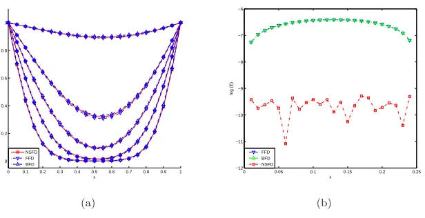
where ˆC(x, s) is the Laplace transform ofC(x, t). Unfortunately, the inverse Laplace transform for ˆC(x, s) is not available. In order to determinate the solution in the time-domain, we have used the numerical inversion by Zakians algorithm [22,24]. We apply new scheme to (3.1) with different values ofP andφ. Several studies indi-cated that numerical results of standard finite difference methods lead to numerical dispersions in the advection dominated problems [5,18,19,25]. Figure 1 shows the concentration profiles and their respective errors. As a expected for a wide range of
P and φ, classical FD schemes provide a bigger approximation errors than the new NSFD scheme and for small values ofP (≤1) andφ, better agreements between the FD schemes and new scheme are observed, see Figure 2(a). However, in this case new scheme performs well, see Figure 2(b).
3.2. Test case 2: Exponential traveling wave. The second test case consists of equation (2.1) forP = 1,Q= 1 and R= 1:
∂C(x, t)
∂t +
∂C(x, t)
∂x −
∂2C(x, t)
0 0.1 0.2 0.3 0.4 0.5 0.6 0.7 0.8 0.9 1 0
0.2 0.4 0.6 0.8 1
x
C
NSFD FFD BFD
(a)
0 0.05 0.1 0.15 0.2 0.25 −7
−6.5 −6 −5.5 −5 −4.5 −4 −3.5 −3 −2.5
x
log (E)
FFD BFD NSFD
(b)
Figure 1. Concentration profiles at different times and logarithm of absolute er-rors withP= 10 andφ= 2.
0 0.1 0.2 0.3 0.4 0.5 0.6 0.7 0.8 0.9 1 0
0.2 0.4 0.6 0.8 1
x
C
NSFD FFD BFD
(a)
0 0.05 0.1 0.15 0.2 0.25 −12
−11 −10 −9 −8 −7 −6
x
log (E)
FFD BFD NSFD
(b)
Figure 2. Concentration profiles at different times and logarithm of absolute er-rors withP= 1 andφ= 0.1.
with initial condition
and boundary conditions
C(0, t) = exp(t), t∈[0, T],
(3.9)
∂C(xmax, t)
∂x =−C(xmax, t), t∈[0, T].
The exact solution is given by
C(x, t) = exp(t−x). (3.10)
In order to show the advantages of the proposed new method, we numerically solve (3.7) forxmax = 10 and T = 0.85 using ∆x= 0.1 and ∆t = 0.005. In addition to comparing the solution of the new scheme with the exact solution, we also compare it to the numerical solution produced by a standard upwind forward Euler finite difference method (EE)
Cjn+1−C n j
∆t +
Cn j −C
n j−1
∆x −
Cn
j−1−2Cjn+C n j+1
∆x2 =−C
n
j, (3.11)
and by the nonstandard finite-difference (NSFD) method, proposed by Mickens in [14]
Cjn+1−Cjn
∆t +
Cn
j −Cjn−1
∆x −
Cn
j−1−2Cjn+Cj+1n
∆x2 =−C
n+1
j , (3.12)
using the same values for the parameters. As can be seen from Figure 3, the proposed method is stable and produces a solution that is very close to the exact solution, but both EE and NSFD methods are unstable for this choice of a time step ∆t = 0.005 and larger.
3.3. Test case 3: Colonization of Europe by oaks. In the third test case, we deal with the model for the recolonization by oaks of Europe after the last glaciation. The model assumes Malthusian growth and a standard advection-diffusion reaction equation for the local densityC(x, t) of oaks at timet
∂C(x, t)
∂t +u
∂C(x, t)
∂x −D
∂2C(x, t)
∂x2 =rC(x, t), (x, t)∈[0, xmax]×[0, T], (3.13)
0 2 4 6 8 10 −4 −3 −2 −1 0 1 2 3 4 Space(x) C(x,T) Exact solution New method NSFD method EE method
(a)Solutions at T=0.85
0 0.2 0.4 0.6 0.8 1 0 5 10 −4 −2 0 2 4 Time(t) Space(x) C(x,t)
(b)Solution of the EE method
0 0.2 0.4 0.6 0.8 1 0 5 10 −0.5 0 0.5 1 1.5 2 2.5 Time(t) Space(x) C(x,t)
(c) Solution of the NSFD method
0 0.2 0.4 0.6 0.8 1 0 5 10 0 0.5 1 1.5 2 2.5 Time(t) Space(x) C(x,t)
(d)Solution of the new method
Figure 3. Solutions for the exponential traveling wave model.
time 0 isM and is concentrated at the origin, the exact solution of this equation is
C(x, t) = M 2√πDtexp
rt−(x−ut)
2
4Dt
, (3.14)
for more details see [4].
In Figure 4 numerical solutions for (3.13) are shown with u = 1, D = 1, r = 0.1,
xmax= 10, T = 2, ∆x= 0.1 and ∆t= 0.005. Comparing the proposed new method with the upwind EE method
Cjn+1−Cjn
∆t +u
Cn
j −Cjn−1
∆x −D
Cn
j−1−2Cjn+Cj+1n
∆x2 =rC
n
j, (3.15)
0 1 2 3 4 5 6 7 8 9 10 −5
0 5 10 15 20 25 30 35 40 45
Space (x)
C(x,T)
Exact solution New method EE method
(a)Solutions at T=2
1 1.2 1.4
1.6 1.8 2
0 5 10 −1 −0.5 0 0.5 1
x 1016
Time(t) Space(x)
C(x,t)
(b)Solution of the EE method
1 1.2
1.4 1.6 1.8
2
0 5 10
0 10 20 30 40
Time(t) Space(x)
C(x,t)
(c) Solution of the new method
1 1.2
1.4 1.6 1.8
2
0 5 10
0 10 20 30 40
Time(t) Space(x)
C(x,t)
(d)Exact solution
Figure 4. Solutions for the oak propagation model.
4. conclusions and discussion
on positivity for the new method. A future work can be investigate the necessity of condition for positivity in Theorem 1.
References
[1] A. Berman, R. J. Plemmons, Nonnegative matrices in the mathematical sciences, Academic Press, New York, (1979).
[2] B. M. Chen-Charpentier, H. V. Kojouharov, An unconditionally positivity preserving scheme for advectiondiffusion reaction equations. Mathematical and computer modelling, 57: 9 (2013), 2177-2185.
[3] W. Hundsdorfer, J. G. Verwer, Numerical Solution of Time-Dependent Advection-Diffusion-Reaction Equation,Springer(2003).
[4] J. Istas, Mathematical Modeling for the Life Sciences, Springer-Verlag, Berlin, (2005).
[5] H. Karahan, A third-order upwind scheme for the advectiondiffusion equation using spreadsheets, Advances in Engineering Software, 38 (2007), 688-697.
[6] M. Mehdizadeh Khalsaraei, An improvement on the positivity results for 2-stage explicit Runge-Kutta methods, Journal of Computatinal and Applied mathematics 235 (2010), 137-143.
[7] M. Mehdizadeh Khalsaraei, F. Khodadoosti, 2-stage explicit total variation diminishing preserv-ing Runge-Kutta methods,Computational Methods for Differential Equations 1(2013), 30-38. [8] M. Mehdizadeh Khalsaraei, F. Khodadoosti, A new total variation diminishing implicit
non-standard finite difference scheme for conservation laws, Computational Methods for Differential Equations, 2 (2014), 85-92.
[9] M. Mehdizadeh Khalsaraei, F. Khodadoosti, Nonstandard finite difference schemes for differential equations. Sahand Commun. Math. Anal, Vol. 1 No. 2 (2014), 47-54.
[10] M. Mehdizadeh Khalsaraei, F. Khodadoosti, Qualitatively stability of nonstandard 2-stage ex-plicit Runge-Kutta methods of order two. Computational Mathematics and Mathematical physics. In press.
[11] M. Mehdizadeh Khalsaraei, Positivity of an explicit Runge-Kutta method. Ain Shams Engineer-ing Journal. In press.
[12] R. E. Mickens, Exact solution to a finite difference model of a nonlinear reaction-advection equation: implications for numerical analysis. Numer. Meth. Part. D. E. 5 (1989), 313-325. [13] R. E. Mickens, Nonstandard Finite Difference Models of Differential Equations. World Scientific,
Singapore (1994).
[14] R. E. Mickens, Nonstandard finite difference schemes for reactiondiffusion equations having linear advection, Numer. Methods Partial Differential Equations. 16: 4 (2000), 361364.
[15] R. E. Mickens, A nonstandard finite difference scheme for a Fisher PDE having nonlinear dif-fusion. Computer and Mathematics with Applications, 45 (2003), 429-436.
[16] R. E. Mickens, P. M. Jordan, A positivity-preserving nonstandard finite difference scheme for the Damped Wave Equation. Numer Methods Partial Differential Eq. 20 (2004), 639-649. [17] R. E. Mickens, P. M. Jordan, A new positivity-preserving nonstandard finite difference scheme
for the DWE. Numer Methods Partial Differential Eq. 21 (2005), 976-985.
[19] B. J. Noye, H. H. Tan, Finite difference methods for the two-dimensional advection diffusion equation. Int J Numer Meth Fluids, 9 (1989), 7598.
[20] C. W. Shu, Total-variation-diminishing time discretizations, SIAM J. Sci. Statist. Com- put. 9 (1988), 1073-1084.
[21] G. D. Smith, Numerical Solution of Partial Differential Equations: Finite Difference Methods. Oxford University Press, Oxford (1985).
[22] O. Taiwo, J. Schultz, V. Krebs, A comparison of two methods for the numerical inversion of Laplace transform. Comput. Chem. Eng. 19 (1995), 303-305.
[23] G. Windisch, M-matrices in Numerical Analysis. Teubner-Texte zur Mathematik, 115, Leipzig, (1989).
[24] V. Zakian, Properties of IMN and JMN approximates and applications to numerical inversion of Laplace transforms and initial value problems. J. Math. Anal. Appl. 50 (1975), 191-222. [25] C. Zheng, G. D. Bennett, Applied contaminant transport modeling. New York: Int. Thomson